Walkie-Markie: Indoor Pathway Mapping Made Easy
←
→
Page content transcription
If your browser does not render page correctly, please read the page content below
Walkie-Markie: Indoor Pathway Mapping Made Easy

      Guobin Shen,† Zhuo Chen,‡ Peichao Zhang,‡ Thomas Moscibroda,† Yongguang Zhang†
                             Microsoft Research Asia, Beijing, China
        † {jackysh, moscitho, ygz}@microsoft.com, ‡ {czxxdd, starforever00}@gmail.com

Abstract                                                            gathering processes that map radio signals onto an indoor
                                                                    map that geographically reflects the physical layout of
We present Walkie-Markie – an indoor pathway map-                   the building. Several recent efforts aimed at alleviating
ping system that can automatically reconstruct internal             the pain of radio map construction require knowledge of
pathway maps of buildings without any a-priori knowl-               the real floor plans [26, 38]. Similarly, tracking based lo-
edge about the building, such as the floor plan or access           calization also requires accurate indoor maps (e.g., floor
point locations. Central to Walkie-Markie is a novel ex-            plans or pathway maps) to constrain the drifting of in-
ploitation of the WiFi infrastructure to define landmark-           ertia sensors [36, 37]. Such indoor maps are difficult to
s (WiFi-Marks) to fuse crowdsourced user trajectories               obtain in general, as they may belong to different own-
obtained from inertial sensors on users’ mobile phones.             ers, may be outdated, and many legacy buildings simply
WiFi-Marks are special pathway locations at which the               do not have them at all.
trend of the received WiFi signal strength changes from
                                                                       In this paper, we try to fundamentally rethink the as-
increasing to decreasing when moving along the path-
                                                                    sumption and ask the question: can we build an indoor
way. By embedding these WiFi-Marks in a 2D plane us-
                                                                    map without any prior knowledge about the building? In
ing a newly devised algorithm and connecting them with
                                                                    particular, we are interested in building pathway map-
calibrated user trajectories, Walkie-Markie is able to in-
                                                                    s because they provide a natural framework for localiz-
fer pathway maps with high accuracy. Our experiments
                                                                    ing users and points of interest (POIs) as people usually
demonstrate that Walkie-Markie is able to reconstruc-
                                                                    move along pathways and indoor POIs are connected vi-
t a high-quality pathway map for a real office-building
                                                                    a pathways. A pathway map can also serve as the basis
floor after only 5-6 rounds of walks, with accuracy grad-
                                                                    for other maps specific to other localization approaches,
ually improving as more user data becomes available.
                                                                    or can be used as a building block to construct seman-
The maximum discrepancy between the inferred path-
                                                                    tically richer maps for users, for example through auto-
way map and the real one is within 3m and 2.8m for the
                                                                    matic location detection (e.g., [3]) or crowdsourced user
anchor nodes and path segments, respectively.
                                                                    annotation. Finally, we seek a technology that allows to
                                                                    obtain such pathway maps at scale, say for millions of
1   Introduction                                                    buildings across the world, including shopping malls and
                                                                    office buildings.
Accurate and inexpensive indoor localization is one of                 We address these problems in Walkie-Markie, a sys-
the holy grails of mobile computing, as it is the key to en-        tem that automatically generates indoor pathway maps
abling indoor location-based services. Despite very sig-            from traces contributed by mobile phone users. The sys-
nificant research effort, relatively little has actually been       tem uses crowdsourcing to generate the pathway map of
deployed at scale. One reason is that a common and crit-            unknown buildings without requiring any a-priori infor-
ical assumption of existing approaches – the availabil-             mation such as floor-plans, any initial measurements or
ity of a suitable localization map – is hard to fulfill in          inspection, and any instrumentation of the building with
practice. For instance, WiFi triangulation or fingerprint-          specific hardware. The only assumption Walkie-Markie
ing based approaches for indoor localization rely on a              requires is that there exists a WiFi infrastructure in the
priori AP position information, or a signal strength map            building that is to be mapped. AP locations do not need
to function properly [4, 13, 24]. Such maps are typical-            to be known; instead APs must merely exist for the sys-
ly constructed via dedicated, often labor-intensive, data-          tem to work.

                                                                1
USENIX Association              10th USENIX Symposium on Networked Systems Design and Implementation (NSDI ’13) 85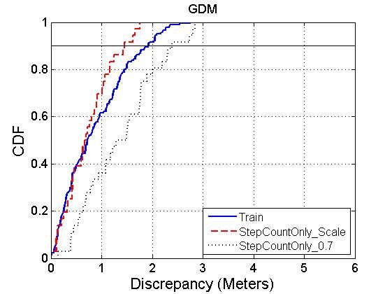
Walkie-Markie is based on two key observations.                 location-invariant, WiFi-Marks yield the common refer-
First, a modern mobile phone can dead reckon the us-               ence points for fusing snippets of user trajectories. With
er’s movement trajectory from its inertial measurement             more user trajectories, the noise tend to cancel each out,
units (i.e., IMU sensors, including accelerometer, mag-            which leads to more accurate displacement measurement
netometer and gyroscope) [21,26,28,36]. The idea is that           between WiFi-Marks. Thus, mapping accuracy gradual-
if sufficiently many users walk inside a building and re-          ly improves as more data becomes available. IMU-based
port their trajectories, we can infer the pathway map. The         tracking suffers notoriously from rapid error accumula-
challenge is that IMU-based tracking is accurate only ini-         tion as distance increases. WiFi-Marks also help with
tially as it suffers from severe drift: rapid error accumu-        the drift problem of IMU-based tracking by bounding
lation over time. Moreover, to generate maps at scale via          the distances between which IMU-based tracking must
crowdsourcing, we must deal with trajectories from dif-            be relied upon.
ferent users, who may start their walks from anywhere, at             Another ingredient of Walkie-Markie is a novel graph
different stride lengths, varying speed, etc. Second, WiFi         embedding algorithm, Arturia, that fixes WiFi-Marks to
networks have been widely deployed, from office build-             “known” 2D locations respecting the constraints sug-
ings to shopping malls. WiFi has been successfully used            gested by the user trajectories. The resulting pathway
by fingerprinting-based localization schemes, and com-             map naturally reflects the physical layout. Arturia dif-
bined WiFi and IMU-tracking solutions have also been               fers from existing embedding algorithms in that it uses
proposed, e.g., [5,11,26,31,38]. However, there are well-          measured displacement vectors as opposed to distances
known practical concerns when using WiFi for localiza-             between nodes as input constraints. After WiFi-Marks
tion: signals fluctuate significantly during different times       are properly placed on the 2D plane, the pathway map
of day, different phones can have different receiver gains         is generated by connecting the embedded WiFi-Marks
(i.e., device diversity) [14,34], and readings also vary de-       with corresponding user trajectories. The obtained path-
pending on how people place their phones e.g., in hand,            way maps can be used by users to localize themselves
in pocket, or in backpack (i.e., usage diversity) [19].            by adding the displacement to the position of the last en-
   Walkie-Markie consists of mobile clients on users’              countered WiFi-Mark. The pathway maps can also be
mobile phones and a backend service in the cloud. When             used to generate other localization maps such as radio
participants walk, the client collects the rough trajectory        maps.
information (step count, step frequency, and walking di-              We have implemented Walkie-Markie and evaluated it
rection) as well as periodic WiFi scan results. The back-          in an office building and a shopping mall. Our experi-
end service fuses these possibly partial user traces (w.r.t        mental results show that we can achieve mapping accu-
the overall internal pathways) and generates the pathway           racy within 3 meters by merging enough user trajecto-
map.                                                               ries (each as short as one minute) equaling to 5-6 rounds
   Central to Walkie-Markie is the WiFi-defined land-              of walking. The mapping accuracy gradually improves
mark (WiFi-Mark), which is a novel way to exploit the              and stabilizes after about 1-2 times more walking time
widely-deployed WiFi infrastructure to establish accu-             along the same paths. Additional experiments on local-
rate and stable landmarks, which serve to anchor the var-          ization using pathway as well as radio maps produced
ious partial trajectories. A WiFi-Mark is defined as a             by Walkie-Markie show that the average and 90 per-
pathway location at which the trend of received signal             centile localization errors are 1.65m and 2.9m, respec-
strength (RSS) from a certain AP reverses, i.e., changes           tively, when using displacement from the last WiFi-Mark
from increasing to decreasing, as the user moves along             using the pathway map.
the pathway. We show in this paper that such WiFi-
Marks based on the RSS trend (instead of the face RSS              2   Problem and Challenges
value used in previous works) overcomes the aforemen-
tioned challenges in leveraging WiFi signals and yields            Problem Statement: Indoor localization results are
highly stable and easily identifiable landmarks. WiFi-             meaningful only when associated with corresponding in-
Marks are determined by the relative physical layout of            door maps (e.g., pathway maps) that geographically re-
the AP and the pathway, and are thus location invariant.           flect the physical layout. However, in this context the
Moreover, a single AP often leads to multiple uniquely             availability of such maps has largely been taken for
identifiable WiFi-Marks, leading to a higher density of            granted, often via assumptions. For instance, IMU-based
WiFi-Marks.                                                        tracking and localization systems have assumed accu-
   WiFi-Marks allow us to overcome two key problem-                rate indoor maps (e.g., floor plans) to constrain drifting;
s in mapping buildings: i) merging the large volumes               WiFi-based localization systems further assume a-priori
of crowdsourced (partial) trajectories and ii) bounding            knowledge about AP positions or a radio signal map
the tracking error and drift of IMU sensors. Being                 [4,13,24]. While there are many existing works trying to

                                                               2
86 10th USENIX Symposium on Networked Systems Design and Implementation (NSDI ’13)                        USENIX Association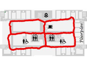
reduce the dependency on such a-priori information (AP
locations [6], radio signal map [12, 16, 22, 26, 38]), they
all assume a known internal map of the floor, which are
often not readily available.
   In this paper, we remove this assumption and build an
indoor pathway mapping systems without assuming any
prior knowledge of the building. Our goal is to find a so-
lution that works with existing infrastructure, is applica-
ble to commercial mobile phones, and is “crowdsource-
able” so as to scale to a large number of buildings. The
only assumption we make is the mere existence of a WiFi
infrastructure in the buildings to be mapped.
                                                                  Figure 1: Illustration of WiFi-Marks, as determined by
Challenges: Previous work has tried to combine WiFi               the relative physical layout of the AP and the pathways.
signals and IMU sensing data [5,10,11,31]. The problem
with IMU-based technologies is that they can track a us-
er’s trajectory at some accuracy for only a short period of       3.1    WiFi-Marks: Concept
time, and will drift severely as the walking time increas-        Previous work on WiFi-based localization has used the
es. This makes it hard to align multiple trajectories, and        received WiFi signal strength (RSS) directly. It turns out
trajectories obtained from different users (with differen-        that this is the root cause of the aforementioned prob-
t start points) are even harder to combine into a whole           lems. The key insight is that significantly more stable
pathway map. Leveraging WiFi also poses well-known                landmarks can be obtained from an existing infrastruc-
challenges. Even though WiFi fingerprints are statistical-        ture by using WiFi signal strength indirectly: instead of
ly locality-preserving [16, 24], an AP’s coverage area is         looking at the face RSS values, we look at the trend of
overly large for the desired accuracy of a useful internal        RSS changes.
pathway map. Typically, multiple pathways are covered                Figure 1 illustrates the basic idea. A user is walking
by a single AP. The AP’s position is also unknown. Fur-           from left to right along a pathway covered by an AP. Ini-
thermore, other challenges common to WiFi-based lo-               tially we see RSS increase as the user moves closer to-
calization systems are: i) WiFi signal fluctuations due to        wards the AP. When the user walks past the point from
ambient interference, multipath effect, and environmen-           which the distance to AP increases, the RSS trend revers-
tal dynamics such as the time-of-day effect; ii) device di-       es. In theory, this RSS trend tipping point (RTTP) should
versity with different receiver gains at different phones;        correspond to a fixed position on the pathway that is clos-
and iii) device usage diversity caused by people placing          est to the AP in terms of signal propagation.
their phones differently such as in hand, in pocket, in
                                                                     The key appeal of examining the RSS trend instead
purse, or in a backpack. We note that usage diversity is
                                                                  of taking individual RSS readings is that it may solve
rarely mentioned in the literature, but is a real impairing
                                                                  the device and usage diversity problems: no matter what
factor.
                                                                  make and model of the phone, what time of the day, and
                                                                  how the phone is kept with respect to its user, the RTTP
                                                                  should occur at around the same location. Through de-
3   WiFi-defined Landmark                                         tailed experiments, we argue in Section 3.3 that locations
                                                                  where the RSS trend of a certain AP changes are excel-
In real life, landmarks are often used to give directions.        lent candidates for landmarks. We call these points WiFi-
No matter how one detours, once a landmark is encoun-             defined landmark, or short WiFi-Marks (WM) hereafter.
tered, previous errors are reset. Using the same idea, we
can leverage landmarks to constrain the drifting in IMU           3.2    WiFi-Marks: Identification
tracking, and to align different user trajectories. Howev-
er, the challenge is the find landmarks that are perceiv-         As a landmark, each WiFi-Mark should be uniquely i-
able by mobile phones without human intervention. S-              dentifiable. Depending on how the coverage area of an
ince mobile phones can sense the WiFi environment in              AP intersects with the pathways, it is possible and in fac-
the background, we would ideally like to identify land-           t quite likely that one AP will generate multiple WiFi-
marks based on WiFi signal. In this section, we show              Marks (see Figure 2). Hence while BSSID (the MAC
that–using the concept of WiFi-Marks–this is indeed pos-          address of the AP) can uniquely identify the master AP,
sible in spite of the multitude of challenges mentioned           it alone is insufficient to uniquely identify a WiFi-Mark
above.                                                            since there can be multiple pathways under the cover-

                                                              3
USENIX Association             10th USENIX Symposium on Networked Systems Design and Implementation (NSDI ’13) 87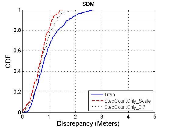
age of the same AP. Therefore, we need to use additional        turning styles. To further differentiate such RTTPs, we
information to differentiate different WiFi-Marks of the        leverage neighborhood AP information. In the same ex-
same master AP.                                                 ample, RTTP 2 may see AP2 only and RTTP 3 sees AP3
                                                                only. Even if they see the exact same set of APs, there
                                                                is still a good chance that the relative RSS values will
                                                                be different due to the difference in distance to each AP.
                                                                Note that it is important to use the RSS differences to
                                                                the master AP’s RSS instead of their real RSS values to
                                                                avoid the device diversity problem. From the radio prop-
                                                                agation model [1], it can be verified that RSS differences
                                                                between multiple APs are not affected by the receiver
                                                                gain for a device.
                                                                   Due to sensing noise, D1 , D2 , and N of a given WiFi-
                                                                Mark can be slightly different each time the WiFi-Mark
                                                                is measured. Therefore, we employ a WiFi-Mark cluster-
                                                                ing process (see Section 6). There are further unreliable
Figure 2: Possibly multiple WiFi-Marks for the same AP.         RTTP detections, such as when a user is not walking s-
                                                                traight or steadily (e.g., zigzagging) or when the phone’s
  In Walkie-Markie, we identify a WiFi-Mark by the fol-         position changes rapidly (e.g. taken out of the pocket).
lowing three-tuple:                                             Our system therefore accepts an RTTP as a WiFi-Mark
            W M  {BSSID, (D1 , D2 ), N }                       only if the IMU sensor indicates a stable walking mo-
                                                                tion and no U-turn is detected during the measurement
where BSSID is the ID of the master AP, D1 and D2 are           process.
the steady walking directions approaching and leaving
the RTTP, respectively. They can be obtained from the
phone’s magnetometer. N is the set of neighboring AP-           3.3   WiFi-Marks: Stability
s’ information, including their BSSID and the respective        Evaluation Scenarios: The indoor radio environmen-
RSS differences to that of the master AP.                       t is complex and often deviates significantly from ideal
   The walking direction information (D1 , D2 ) is adopt-       propagation models. To verify the stability of the RTTPs
ed to differentiate pathways and turns. For example, Fig-       in practice, we conduct the experiments using different
ure 3 shows the possible RTTPs for AP1 , under different        devices (HTC G7, Moto XT800, and Nexus S), at differ-
walking patterns. With directions, we can readily dif-          ent time of day (morning, afternoon, evening, and mid-
ferentiate RTTP 1, {2,3}, 4, and 5. In addition, the di-        night), and with the phones held at different body posi-
rection can be used to disqualify some erroneous RTTP           tions (hand, trouser pocket, purse, and backpack). All
detections when the user makes a U-turn (e.g., RTTP 6           of these are important factors affecting RSS. In addition,
and 7). Not identifying such “U-turn RTTPs”, could add          we perform experiments in two buildings to demonstrate
significant noise to the system.                                the generality of our approach.
                                                                   We present two sets of experiments. In the first set,
                                                                we walk and wait, i.e., wait to ensure a complete scan
                                                                of all WiFi channels before walking to a next collection
                                                                point. This represents an ideal case. In the second set,
                                                                we walk continuously at slow or normal speed without
                                                                waiting for WiFi scans to complete. Figure 4 shows the
                                                                curves of collected RSS values and the locations of the
                                                                detected WiFi-Marks. From the figure, we can see that
                                                                the RSS values from different devices are evidently d-
                                                                ifferent, and the same is true for the same device at d-
                                                                ifferent time of day, or at different body positions. In
                                                                contrast, the increasing and decreasing RSS trends are
Figure 3: Multiple RTTP possibilities for AP1 under dif-        always easily identifiable, and the WiFi-Mark positions
ferent walking patterns illustrated by arrows.                  are not only highly clustered and stable, but also consis-
                                                                tent between the two devices. Taking the normal walk-
  RTTPs with similar (D1 , D2 ) can arise from parallel         ing case as an example, the average position deviations
corridors (e.g., RTTP 2 and 3 in Figure 3) or similar           are 1.3m and 2.9m for Moto XT800 and Nexus S, re-

                                                            4
88 10th USENIX Symposium on Networked Systems Design and Implementation (NSDI ’13)                    USENIX Association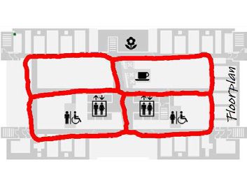
(a) Walk and wait.                         (b) Slow walking.                           (c) Normal walking.
Figure 4: RSS curves for one AP along a corridor using two phones. Blue dotted lines and red solid lines are the raw
and filtered RSS curves (see Section 6). Multiple same type of lines are measurement from different time of day. In
(a), all phones were held in hand. In (b) and (c), Moto was held in hand and Nexus S in trouser pocket.

spectively, while the mean center position offset is only        motion states periodically. When the user is detected in
2.7m between devices. In the ideal case, the deviations          walking state, IMU-based tracking is activated and the
are even better. The reason is that because of the rela-         instantaneous walking frequency and direction of each
tively long WiFi scanning time in today’s mobile phone           step is recorded for displacement estimation. At the same
(usually about 1.5s), the user may have already walked a         time, WiFi signal scanning is performed opportunistical-
few steps during a scan.                                         ly. If a WiFi signal is detected and the device has not
   Stability Evaluation: We also conduct controlled ex-          associated with an AP, the WiFi-Mark detection process
periments in larger areas with more pathways, still using        is activated. Information about the detected WiFi-Marks
various devices and walking at various speeds and at dif-        and estimated displacements between neighboring WiFi-
ferent times of day. For each different setting we collect       Marks are stored, and later sent to the backend service.
data over 5 rounds and calculate the statistical deviation          The Walkie-Markie backend service listens to WiFi-
in WiFi-Mark position. We note that the peak RSS value           Mark updates from all clients. Upon receiving WiFi-
at RTTPs are not all strong, some being as weak as -75           Mark updates, it examines if their master APs are new
dBm.                                                             or already existing. Updates with new master APs are
   Figure 5-(a) shows the cumulative distribution func-          recorded and aged to mitigate the impact of transient APs
tion (CDF) of the deviations for the different settings.         (e.g., mobile APs). For existing ones that are old enough,
We can see that for over 90% of WiFi-Marks, the devia-           their neighborhood consistency is further checked to en-
tions are within 2.5m, and about 70% are within 1.5m in          sure they are not relocated APs, which would be treat-
all cases. We further study whether WiFi-Marks detect-           ed as new APs. Then a clustering process is executed
ed with different settings are consistent, using the cen-        to cluster different detections of the same actual WiFi-
ter offset of WiFi-Mark clusters. Figure 5-(b) shows the         Marks. Each cluster is then assigned one coordinate by
CDF of the center offsets. They are indeed consistent:           the Arturia engine. Finally, with WiFi-Marks positioned
over 95% of the offsets are within 2.5m and over 75%             at the right places and user trajectories connecting them,
are within 1.5m. These results demonstrate that WiFi-            the backend service can generate the desired pathway
Marks are stable and robust across various dimensions,           maps.
and thus have ideal properties to be landmarks for our
indoor pathway mapping purpose.
                                                                 5   WiFi-Mark Positioning

4   Walkie-Markie: Overview                                      WiFi-Marks (or landmarks in general) serve their pur-
                                                                 pose as a reference points only once we can place them
With WiFi-Marks, we now have the common reference                at a known location. For this reason, we need to assign
points for fusing crowdsourced user trajectories together.       coordinates to WiFi-Marks, which is a classical node em-
Walkie-Markie consists of a client–an application run-           bedding problem in the network coordinate and localiza-
ning on users’ mobile phones–and the backend service             tion literature.
running in the cloud. The overall architecture is shown             Distance vs Displacement: Previous node embedding
in Figure 6.                                                     work has unanimously assumed scalar distances (e.g., vi-
   A Walkie-Markie client works as follows: a back-              a direct distance measurement or the shortest path) be-
ground motion state detection engine monitors users’             tween nodes [9, 23, 30]. However, in our case, users may

                                                             5

USENIX Association               10th USENIX Symposium on Networked Systems Design and Implementation (NSDI ’13) 89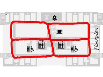
CDF of detected WM location deviation CDF of detected WM location differences
100% 100%
80% 80%
Percentage
Percentage
60% 60%
40% 40%
20% Scan @ slow moving speed, HTC G7 20% Different devices @ normal moving speed
Scan @ slow moving speed, Nexus S Different devices @ slow moving speed
Scan @ normal moving speed, HTC G7 Different walking speed @ HTC G7
Scan @ normal moving speed, Nexus S Different walking speed @ Nexus S
0% 0%
0 1 2 3 4 5 0 1 2 3 4 5
Standard deviation (Meters) Defference (Meters)
(a) CDF of WM position deviation (b) Consistency of WM positions
Figure 5: Statistics on WM positions. Figure 6: Walkie-Markie system architecture.
not always take the shortest path and, in fact, the internal there exists a real user trajectory in between. The rest
floor layout may even prevent people from taking short- length of the spring (i.e., the constraint) is the real dis-
est paths (e.g., two nearby WiFi-Marks blocked by a wall placement measurement from user trajectory. Multiple
or a locked door). If multiple paths exist, taking differ- edges between a pair of nodes are possible if there ex-
ent paths will lead to different distances. These factors ist multiple user trajectories. In this way, we ensure that
often lead to severe violations of the triangle inequality, more frequently encountered WiFi-Marks will have more
which lies at the heart of existing embedding algorithm- accurate coordinates as compared with the alternative s-
s. Consequently, using distances between WiFi-Marks trategy that uses a single average edge.
is insufficient and the displacement vector (i.e., both the Realizing the Graph: With the spring network, our
distance and the direction, obtainable from IMU sensors) goal is to minimize the overall residual potential ener-
between WiFi-Marks has to be used. gy E, which is a function of the discrepancy between
Using direction information in addition to distance the calculated distance (i.e., actual length of the spring)
is fundamental, because it can largely avoid the “fold- and the real measurement (i.e., rest length of the spring).
freedom” problem of the embedding process [25], and Our solution is to adjust the node’s position as if it were
dismiss flip and rotational ambiguities. The only remain- pushed or pulled by a net force from all connecting
ing translational ambiguity can be fixed by fixing any an- neighboring springs. Arturia works as follows:
chor point with an absolute location (e.g., entrances or Initialization: We may randomly assign all nodes’s
window positions of a building with GPS readings). In initial coordinates, or simply to the origin. But for up-
addition, using direction information also requires few- dates due to new incoming data, the previous coordinates
er measurements: only N unique displacement measure- are used for faster convergence and better consistency,
ments are required to localize N WiFi-Marks, whereas i.e., minimal adjustment to the previous graph.
3N − 6 unique measurements would be required when Iteration: At each iteration, adjust the coordinates for
using distances only (in which case the results would still each node according to the compound constraints of the
suffer from flip and rotational ambiguities). Thus, using neighboring nodes. Let p̂i be the current coordinate of
displacement vectors enables faster bootstrapping and is node i. We have d i, j = p̂i − p̂ j as the current displace-
highly desired for a crowdsourcing system. ment vector between node i and a neighboring node j.
Assume there are Ne,i, j real measurement constraints
between node i and j, and let ri, j,k be the kth constraint.
5.1 Arturia Positioning Algorithm Then the adjustment vector is calculated as
In our system, a major challenge is the inaccuracy of Ne,i, j
IMU-based displacement measurements (e.g., errors in εi, j = ∑ ( ri, j,k − d i, j ) (1)
stride length and/or direction estimation). To compen- k=1
sate these errors, we design a new embedding algorith- The gross adjustment vector Fi is obtained by summing
m, Arturia, that handles noisy IMU measurements and up εi, j over all neighboring nodes, i.e., Fi = ∑ j εi, j . Then,
assigns optimal coordinates to WiFi-Marks. Arturia is node i’s coordinate is updated as p̂i = p̂i + Fi .
based on the spring relaxation concept, where each edge The step size of the adjustment (i.e., | Fi |) plays a criti-
of the graph is assumed as a spring and the whole graph cal role in the convergence speed: large adjustment steps
forms a spring network. may lead to oscillation while small adjustments will con-
Building the Graph: An edge (hence, a spring) is verge slowly, as also observed in [9]. To obtain a suitable
added between two specific WiFi-Mark nodes as long as step size, we empirically amortize the adjustment vector
6
90 10th USENIX Symposium on Networked Systems Design and Implementation (NSDI ’13) USENIX Association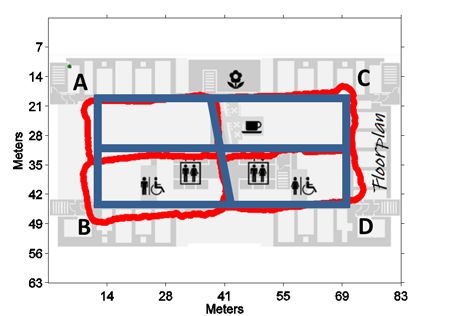
according to Ne,i , the total number of edges to all neigh- Figure 8). We see that after 100 iterations, the nodes are
bors of node i. That is,
Fi = N1e,i ∑ j
εi, j . still heavily folded in Vivaldi. AFL is better than Vivaldi
Termination: For each node i, the local residual po- in shape, but at a wrong scale. For Arturia, the nodes are
tential energy Ei is calculated as Ei = ∑ j |
εi, j |2 . System almost in correct positions after only 30 iterations.
residual potential energy is then E = ∑i Ei . This value
tends to increase with additional edges of the spring net-
work. To obtain a universally applicable termination cri-
terion, we use the normalized potential energy Ē = E/Ne
with Ne being the total number of constraining edges.
The iteration will terminate when the change of Ē fall-
s below a small pre-determined threshold.
Algorithm Comparison: The spring relaxation con- Ground Truth Vivaldi, K = 100
cept has previously been adopted, e.g. in [9, 15, 25]. The
major difference is that the local adjustment (i.e.,
Fi ) in
each iteration has direction information and will always
move closer to the target coordinates in Arturia. This is
not the case in other algorithms where the moving direc-
tion is calculated based on the noisy, intermediate coordi-
nates. Figure 7 illustrates this difference between Arturia
and the Vivaldi [9] algorithm for an intermediate adjust- AFL, K = 100 Arturia, K = 30
ment step to Node 3. We can see that in Arturia, the net
force of the adjustment points directly to Node 3’s target Figure 8: Snapshots of node positions at the different
position, while in Vivaldi it does not. The reason is that iterations for Vivaldi, AFL and Arturia.
the constraints in Arturia are displacement vectors (e.g.,
r3,1 and
r3,2 ) with direction information, while in Vivaldi Speed and Accuracy: We study the convergence speed
they are scalar distances (e.g., |
r3,1 | and |
r3,2 |). and the resulting accuracy of different algorithms by
varying the parameters N and n. Each experiment is re-
peated 10 times and average results are reported. Note
that in the simulation, we have used the magnitude of
displacement as the distance for Vivaldi and AFL to en-
sure the obeyance of triangular inequality, i.e., all nodes
are mostly localizable.
The speed is measured as the number of iterations. For
the accuracy metric, we adopt the Global Energy Ratio
(GER) because it captures the global structural proper-
Figure 7: Illustration of an intermediate adjustment step ty [25]. GER is defined as the root-mean-square nor-
of Vivaldi [9] and Arturia. malized error value of the node-to-node distances, i.e.,
GER = Σi, j:i< j ε̂i2j /(N(N − 1)/2) where N is the total
node number and ε̂i j = |∆d
i j |/|d
i j | is the normalized n-
5.2 Arturia Evaluation ode distance error.
Table 1 shows the results. We see that the proposed
We evaluate Arturia with simulations. We randomly de-
Arturia algorithm is significantly better than the oth-
ploy N nodes in a 100 × 100 square area. For each node,
er two algorithms in terms of both convergence speed
we build n edges to n random neighboring nodes. For
and accuracy. In general, with higher connectivity, both
each edge, the direction is adjusted by a random number
speed and accuracy improve for all three algorithms.
within ±30 degrees, while the distance (i.e., the mag-
This is due to larger damping effects resulting from more
nitude of displacement) is randomly adjusted by within
densely interconnected springs. However, even with
±10 percent. These numbers reflect the real displace-
dense connectivity, the accuracy of Vivaldi is poor be-
ment estimation error ranges.
cause of heavy folding. AFL works better by finding
Anti-folding Capability: As mentioned, using direc- better initial positions. In our target scenario, the node
tion helps to avoid “fold-freedom” issues. We demon- connectivity cannot go very high since there will rarely
strate this by comparing the snapshots of intermediate be direct displacement measurements between faraway
steps of Arturia against those of Vivaldi and AFL (see WiFi-Marks. This highlights the advantage of Arturia in
7
USENIX Association 10th USENIX Symposium on Networked Systems Design and Implementation (NSDI ’13) 91Speed (Iterations) Accuracy (GER) Interestingly, leveraging common WiFi-Marks among
N n
Viv. AFL Art. Viv. AFL Art. user trajectories, we can avoid the error-prone stride
length estimation and instead rely on simpler and more
4 319k 193k 763 .687 .241 .0091
100 6 38k 27k 450 .660 .106 .0072
robust step counting under regular walking, which can be
8 11k 2244 232 .615 .015 .0061 easily be done from the regularity of the IMU data. We
10 6954 971 170 .614 .012 .0056 first randomly select a user and treat her stride length as
4 340k 334k 1552 .745 .279 .0068 the benchmark unit (BU). We then normalize other user-
200 6 42k 19k 706 .736 .060 .0053 s’ stride against hers using partial trajectories between
8 20k 3299 441 .710 .012 .0049 common WiFi-Marks and obtain a normalization factor
10 10k 1552 339 .699 .010 .0046 θ . This normalization process is transitive. Ultimately
all users will normalize their traces to the same BU and
Table 1: Speed and Accuracy comparison of Vivaldi, obtain their respective θ s. Then we obtain the average
AFL, and Arturia. N is the node number and n is the normalization factor θ̄ . The product of θ̄ and the BU will
node connectivity degree. be the real stride length of the “average” user, to which
we can assign the demographic average stride length.
Walking Direction Estimation: We use the magne-
the context of Walkie-Markie.
tometer and the gyroscope to obtain the walking direc-
tion and the turning angles, similar to [18, 21]. Unlike
step detection and stride length that is determined on a
6 System Implementation
per-step basis, the direction of each step needs to be de-
termined by considering those of neighboring steps be-
We have implemented the Walkie-Markie system, with
cause magnetometer readings are sometimes not stable
mobile client on Android phones and backend services
due to disturbance of local building construction or ap-
as Web Services. In this section, we detail a few key
pliances, and the gyroscope may drift over time. In our
components.
implementation, we simply discard portions of magne-
WiFi-Mark Detection: In mobile client, the collected tometer data where drastic changes occur, and rely on the
RSS value is first smoothed over a 9-point weight win- gyroscope to decide whether there is a direction change
dow in a running fashion to detect WiFi-Marks. The in that period. For the portions with stable magnetometer
weight window is empirically set as a triangle function readings, we use a Kalman Filter to combine the mag-
({0.2, 0.4, 0.6, 0.8, 1, 0.8, 0.6, 0.4, 0.2}). We tested netometer and the gyroscope readings to tell the user’s
other window functions (e.g., cosine, raised cosine) and walking directions.
found not much difference in detection accuracy. Then,
WiFi-Mark Clustering: The backend service receives
the trend detection is done by taking derivatives of the s-
many crowdsourced trajectories and WiFi-Mark report-
moothed RSS curves, i.e., the differences between neigh-
s. Due to sensing noise and user motion, the same ac-
boring points. The consecutive positive and negative s-
tual WiFi-Mark may be reported slightly differently in
pans of the differences are identified and the correspond-
directions (D1 , D2 ) and neighborhood (N ). We design a
ing walking directions are checked. If there are no U-
clustering process to detect the same actual WiFi-Mark:
turns and the trend change is significant as controlled
we first classify reported WMs with the same BSSID us-
via a threshold (e.g., 5 dBm), the point with the peak
ing D1 and D2 . To accommodate sensing noise, the di-
(filtered) RSS during the trend transition is selected as a
rections are considered the same if they are within ±20
WiFi-Mark.
degrees. For those WMs with same BSSID and similar
Displacement Estimation: Displacement between directions, a bottom-up hierarchical clustering process as
WiFi-Marks is estimated from user trajectories by accu- in [6,24] is applied on the neighborhood set N . Initially,
mulating the displacement of each step. Step displace- each WM is one cluster. Then the closest clusters are it-
ment carries stride length and walking direction and is eratively merged if their inter-cluster distance is smaller
captured by IMU sensors. Many techniques exist for than a pre-determined threshold, which is set to 15 dBm
stride length estimation [17, 29, 32]. We chose a simple as recommended in [24].
frequency-based model by Cho et al [7]: stride len = The inter-cluster distance is the average distance
a · f + b with f being the instantaneous step frequen- between all inter-cluster pairs of WMs. The distance
cy, and a, b being parameters that can be trained offline. between two WMs is defined over the RSS of the sensed
However, model parameters are specific to a user’s walk- APs (A ) as follows:
ing conditions, e.g., parameters trained from wearing s-
K
port shoes will not work well when wearing high heels.
Improper parameters will lead to large estimation error.
DN (A
i , A
j ) = ∑ (ain − anj )2 /K
n=1
8
92 10th USENIX Symposium on Networked Systems Design and Implementation (NSDI ’13) USENIX Associationthrough tethering. Relocated APs are detected via neigh-
where A i are the RSS differences (to ensure device indif-
borhood (carried in WiFi-Mark reports) consistency and
ference) between the master AP and neighboring APs at treated as new APs. Second, to mitigate the impact of
W Mi , and K is the total number of unique APs detected outlying WiFi-Marks, e.g., resulting from transient mo-
at the two WMs. For orphan APs appearing in one WM’s bile AP or wrongly detected due to magnetometer mal-
neighborhood but not the other, the RSS difference is set function, we enroll a WiFi-Mark cluster only when it has
to peak RSS of the master AP minus -100 dBm. Finally, a sufficient number of members (e.g., three).
each WiFi-Mark cluster is treated as one node in Arturi- Energy consumption: IMU-sensing consumes little
a and assigned one coordinate. All WiFi-Marks in the energy, especially at low sampling rate (e.g., 10Hz in our
same cluster have the same coordinate. case). Our preliminary test shows that 10Hz IMU sens-
Pathway Map Generation: With WiFi-Marks and con- ing shortens the depletion time of a fully charged battery
necting user trajectories, we design the following expan- from 18.3 hours to 17.8 hours. We reduce data commu-
sion and shrinking procedure to generate the pathway nication to the server by performing step detection and
map systematically. Initially, user trajectories are parti- WiFi-Mark detection entirely on the mobile phone. The
tioned into snippets delimited by WiFi-Marks. Snippet- final communication data rate is about 1KB every 100
s with U-turns are filtered out. The remaining trajecto- steps. Note that it can be delayed and piggybacked on
ry snippets are calibrated by proportionally adjusting the other network sessions. The major energy consumption
length and direction of each step using the WiFi-Marks’ is from WiFi scanning. To work around, our client trig-
coordinates assigned by Arturia (affine transformation). gers WiFi scanning only when the user is walking (de-
For each calibrated trajectory snippet, we first draw it on tected from low duty cycled IMU sensors), and we task
a canvas and further expand it to a certain width (i.e., a user to collect just a few minutes of walking data. As
from line to shape). Pixels being occupied are weighted shown in Section 7, even short trajectories can still be
differently according to their distances to the center line: used to infer pathway maps.
the closer the pixels, the higher the weight. Due to the
multiplicity of user trajectories, there may exist multiple
7 Walkie-Markie System Evaluation
snippets connecting the same two WiFi-Marks. Thus,
expanded snippets will overlay together and the weight
of overlapping pixels are summed up. The expansion 7.1 Visual Comparison
process will result in a fat pathway map. A shrinking Before presenting quantitative evaluation results, we first
process is then applied to prune away those outer pixels visually examine the inferred pathway map with the
whose weights are less than a threshold. As some WiFi- ground truth or reference floor plan. This will give us
Marks may be encountered more frequently than others, a general feel for Walkie-Markie’s practicality.
we adapt the threshold as a percentage to the maximum
weight in the local neighborhood. Finally, we remove An Office Floor: We first show the study in our office
isolated pixels and also smooth the edges of the resulting floor for which we have the groundtruth floor plan. The
shrunk pathway map. internal layout consists of meeting rooms, offices, cubi-
cle areas, and relatively large open areas in the middle.
Note that the pathway map generated from above
The experiment floor size is 3,600m2 and the total inter-
expansion-shrinking process is a bitmap. It is also pos-
nal pathway length is 260m. Figure 9 shows the aligned
sible to generate a vector pathway map as all the turns
user trajectories and the inferred pathway maps under d-
can be effectively determined from user trajectories. We
ifferent amounts of user trajectory data. The stars in user
adopt bitmap in this paper for its immediacy in visually
trajectories are the detected WiFi-Marks. As expected,
reflecting the quality of users’ trajectories.
the quality of the resulting pathway map improves with
Practical Considerations: In our implementation, we more user data. After 50 minutes of random walk, the re-
have considered other important issues to build a practi- sulting map is already very close to the real map shown
cal crowdsourcing system. in the bottom-left figure.
Robustness: We have designed two mechanisms to im- A Shopping Mall Floor: We also study a nearby shop-
prove the robustness of the system. First, the backend ping mall. There is no managed WiFi LANs, but many
service implements an enrollment selection mechanis- isolated WiFi islands deployed by coffee shops or from
m. WiFi-Marks from new master APs are recorded and POS machines. The floor has an irregular layout and the
will be incorporated into the Arturia positioning engine internal pathway length is roughly 310m. We walked
only when the AP becomes sufficiently aged. This is about 10 rounds for about 40 minutes with a Nexus S
to counter transient WiFi-Marks, e.g., those caused by phone. The results are shown in Figure 10. The first t-
mobile APs or WiFi hotspot created on mobile phone wo figures show the raw IMU-tracked user trajectories
9
USENIX Association 10th USENIX Symposium on Networked Systems Design and Implementation (NSDI ’13) 9340 40 40 40
30 30 30 30
20 20 20 20
meters
meters
meters
meters
10 10 10 10
0 0 0 0
−10 −10 −10 −10
−20 −20 −20 −20
−10 0 10 20 30 40 50 60 70 80 −10 0 10 20 30 40 50 60 70 80 −10 0 10 20 30 40 50 60 70 80 −10 0 10 20 30 40 50 60 70 80
meters meters meters meters
7 7 7
14 14 14
21 21 21
28 28 28
Meters
Meters
Meters
35 35 35
42 42 42
49 49 49
56 56 56
63 63 63
14 28 41 55 69 83 14 28 41 55 69 83 14 28 41 55 69 83
Meters Meters Meters
(a) after 20min walk. (b) after 30min walk. (c) after 50min walk. (d) after 100min walk.
Figure 9: Aligned user trajectories and generated pathway maps at different amount of user trajectories.
7
30 30
14
20 20 21
Meters
10 10 28
Meters
Meters
35
0 0
42
−10 −10 49
−20 −20 56
63
0 20 40 60 80 100 120 0 20 40 60 80 100 120 14 28 41 55 69 83 97 110 125 140
Meters Meters Meters
(a) normal IMU-tracking (b) with WM alignment (c) Inferred pathway map (d) Picture from flyer.
Figure 10: The picture and generated pathway map for a real shopping mall.
and those aligned with WiFi-Marks. The third figure map. Results reported below are averaged over 10 such
shows the inferred pathway map. Unable to obtain a experiments.
groundtruth floor plan, we took a picture of an emer- Performance Metrics: To quantify the quality of the in-
gency guidance map and highlighted the pathways in the ferred pathway map, we use the following metrics.
last figure. We see that the pathway map generated by
Walkie-Markie is visually very close to the real one. • Graph Discrepancy Metric (GDM): This metric re-
flects the differences in the relative positioning among
anchor nodes, i.e. singular locations such as crosses
7.2 Quantitative Evaluation or sharp turns. Like GER, we compare the Euclidean
distances among all node pairs using coordinates from
We conduct experiments in our office building, for which
respective maps.
we have the groundtruth floor plan.
• Shape Discrepancy Metric (SDM): This metric quan-
Data Collection: We have collected data from seven tifies differences between the shape of inferred paths
users, six male and one female, with heights range from and real ones. Path segments between corresponding
158cm to 182cm. A stride length model is trained for anchor nodes are uniformly sampled to obtain a series
each user. We asked them to walk normally and cover of sample points. The metric is defined as the distance
all the path segments in each round, but they could start between corresponding sampling points. Note the in-
anywhere. Three phone models (Nexus S, HTC G7, and ferred map needs to be registered to the real map first
Moto XT800) were used. The phones were held in hand by aligning at some anchor nodes.
in front of body, hip-pocket, and also a backpack. In
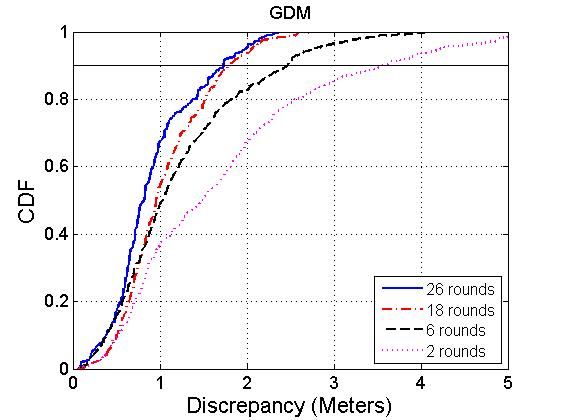
total, the users walked 30 rounds for about two hours. Mapping Accuracy: Figures 11-(a) and (b) show the
In real crowdsourcing scenarios, users may walk on- cumulative distribution (CDF) of GDM from different
ly a portion of all pathways, or we may need to discard amount of trajectory data. We can see that the geometric
portions with irregular walking, or a user may only want layout of all anchors are well preserved with only 2-hour
to be tasked for a short time for consumption of ener- walking data. The maximum difference in distances be-
gy consumption. To simulate these constraints and see if tween corresponding node pairs is about 3 meters, and
short trajectories are still useful, we chop the complete the 90 percentile difference is around 2 meters. We al-
user trajectories into one-minute snippets, and random- so observe that the performance improves as more da-
ly select a certain number of such snippets to infer the ta becomes available. In addition, an accurate pathway
10
94 10th USENIX Symposium on Networked Systems Design and Implementation (NSDI ’13) USENIX Association1 1
0.8 0.8
0.6 0.6
CDF
CDF
0.4 0.4
Anchor A Aligned
100 mins Anchor B Aligned
0.2 0.2
50 mins Anchor C Aligned
30 mins Anchor D Aligned
20 mins Optimal Alignment
0 0
0 1 2 3 4 5 6 0 1 2 3 4 5
Discrepancy (Meters) Meters
(a) Random snippets (a) Intuitive alignments (a) GDM
1
0.8
CDF 0.6
0.4
100 mins
0.2
50 mins
30 mins
20 mins
0
0 1 2 3 4 5
Discrepancy (Meters)
(b) Complete rounds (b) Optimal alignment (b) SDM
Figure 13: System performance using
Figure 11: CDF of GDM. Figure 12: CDF of SDM. step count only.
map can be built from trajectories as short as one-minute minutes of walking data is used, the maximum path dis-
walking, as long as we can obtain sufficiently many of crepancy is within 2.8 meters, and the 90 percentile error
them. is within 1.8 meters.
Comparing the curves with similar walking time (e.g., Step Count Only: We stated above that Walkie-
100min vs 26 rounds) in the two subfigures, we can see Markie can avoid error-prone stride length estimation.
that using complete trajectories leads to better perfor- To verify this claim, we use only the direction and step
mance. This is because chopping the walks into snippets count from the same set of user trajectories. Figure 13
reduces the displacement measurements between WiFi- shows the results. Since we do not know the demograph-
Marks. In general, longer trajectories yields better per- ic average step length, we scale the resulting shape to
formance. best fit the ground truth. This gives the upper bound of
In measuring SDM, we have different options to align system performance. We also simply assign 0.7m as the
the inferred map to the real map to fix the only remaining demographic average step length and obtain the results.
translational ambiguity. In reality, such alignment can be From the figure we can see that even using step count
automatically performed by leveraging user trajectories only leads to high accuracy maps. Comparing with the
that enter or leave the building. Here, we study the results curve using the trained stride length model, we can see
by aligning at any outermost anchor point (e.g., Points A, that the 90 percentile GDM is only slightly worse (with-
B, C, D in the bottom-left figure in Figure 9), and also an in 0.4m) and the 90 percentile SDM is actually better by
optimal alignment at the geometric center of all anchors. about 0.4m.
In all experiments below, we have obtained 10 sample
points on each path segment between two neighboring Impact of AP Density: Our office floor has a relative-
anchors. ly dense AP deployment, about 21 APs covering an area
Figure 12-(a) shows the CDF of SDM using 100 one- of 3,600m2 . It is natural to conjecture that the perfor-
minute snippets. We can see that aligning at different mance of Walkie-Markie may be highly affected by the
points indeed leads to different performance. Neverthe- AP density. To study this impact, we emulate sparse de-
less, the maximum difference among all the five align- ployments by randomly blanking out a certain percent-
ment trials is small, within 1.3 meters. In the remainder age of APs, i.e., eliminating all the WiFi-Marks defined
of the evaluation, we use the optimal alignment. From by those APs and their appearances in other WiFi-Mark’s
Figure 12-(b), we see that the shape of inferred pathways neighbor AP list.
agrees well with the shape of real ones. When over 50 Figure 14 shows the results with varying percentage
11
USENIX Association 10th USENIX Symposium on Networked Systems Design and Implementation (NSDI ’13) 952
GDM (100minutes)
SDM (100minutes)
GDM (50minutes)
SDM (50minutes)
Absolute Error (meter)
1.5
1
0.5
0
20 40 60 80 100
AP percentage
Figure 14: Impact of WiFi AP density. Figure 15: GDM and SDM statistics under different amount of trace data.
of remaining APs. In general, the performance degrades groundtruth positions are also known. We compare the
when the number of AP decreases. But for a dense de- localization results in Figure 16. We can see that Walkie-
ployment like our office building, the number of APs is Markie outperforms RADAR, and more interestingly, the
more than enough for a good result. The result does not localization error is bounded. Quantitatively, the average
suffer if AP density is reduced to 40%. And even a fur- and 90 percentile localization errors are 1.65m and 2.9m
ther reduction to 20% degrade the mapping accuracy on- for Walkie-Markie, and 2.3m and 5.2m for RADAR. We
ly slightly. note that the resulting accuracy is comparable with that
System Agility: We are also interested in learning how reported in Zee [26], and slightly better than that from
agile Walkie-Markie can construct a useful internal path- LiFS [38].
way map. System agility reflects the adaptation capabil-
1
ity to the internal layout changes of a building. It is mea-
sured by the achievable GDM and SDM under different 0.8
amount of user trajectories incorporated into the system.
Figure 15 shows that both discrepancy metrics decrease 0.6
with more data input, and the system converges quick-
CDF
ly: with about 5 to 6 rounds of trajectories (i.e., visits 0.4
per path segment), a highly accurate pathway map can
already be inferred. 0.2
RADAR
Walkie−Markie
8 Application to Localization 0 2 4 6
Localization Error (m)
8 10
Radio Map as Side Product: In Walkie-Markie, WiFi Figure 16: Localization results of Walkie-Markie and
fingerprints are collected when the users walk. When the RADAR in an office floor, using crowd sourced map.
internal pathway map is generated, the position of each
user step can be obtained from the calibrated walking tra-
jectory. With reference to the timestamps of WiFi scans 9 Discussion
and steps, we can easily interpolate the position of each Open Area: Our system works well for normal indoor
WiFi scan. As a result, we can generate a dense WiFi pathways that are typically narrow (say a few meters),
fingerprint map for free. which helps ensuring regular user motion. For large open
Localization: Both the resulting internal pathway map areas, the performance depends on how users walk. If
and the radio map can be used for localization pur- most users walk along roughly the same path (e.g., from
pose. For the former, we can localize a user by track- one entrance to another), Walkie-Markie will still work.
ing the relative displacement since the last WiFi-Mark In general, however, the performance may deteriorate as
encountered, whose position is known. For the latter, users may walk arbitrarily, which will cause noisy WiFi-
we can apply any WiFi fingerprinting-based method such Mark detection and clustering. For wide pathways, the
as the RADAR localization system [4]. For evaluation, inferred map tends to be thinner than the real ones. This
we walked one round along the pathway in the office is because we have assumed a point representation of a
floor. During walking, we ensured every step to be at WiFi-Mark cluster, and we have also assumed the path-
boundaries of carpet tiles. Thus fingerprints are col- way to be around 2-meter wide pruning outer pixels in
lected at half-meter (i.e., the tile size) interval and their the shrinking process. We note that WiFi-Mark clusters
12
96 10th USENIX Symposium on Networked Systems Design and Implementation (NSDI ’13) USENIX Associationfrom wider pathway segments tend to be more diverged than Unloc (e.g., around 10 WiFi landmarks and overal-
than those from thinner ones, we may leverage this fact l 40 landmarks in one building). One recent work [19]
to estimate the pathway width. also exploits the point of maximum RSS, which bears
Multiple Floors: Users may walk across different floors similarity to WiFi-Mark. However, instead of exploiting
using either elevators, escalators, and stairs. These mo- it as a landmark, they use it to switch between two lo-
tion states can be discriminated using accelerometer with cation inference modules. A dedicated training stage is
advanced detection mechanisms [20,35], and can thus be required to obtain the locations of such maximum RSS
excluded in the WiFi-Mark detection. Interestingly, these points. Walkie-Markie builds the pathway map without
functional areas may serve as landmarks as they are sta- pre-training.
ble and reliably detectable via phone sensors. Thus, they There are several papers that combine WiFi and IMU-
can also be incorporated into the Walkie-Markie system, tracking for mapping purpose. WiSLAM [5] seeks to
and treated in the same way as WiFi-Marks by the Ar- construct the WiFi radio map and uses the RSS values
turia engine. To discriminate different functional areas to differentiate different paths. WiFi-SLAM [11] uses
of the same type, we can use the covering WiFi APs. a Gaussian process latent variable model to build WiFi
signal strength maps and can achieve topographically-
Dedicated Walking vs Crowdsourcing: While Walkie- correct connectivity graphs. SmartSlam [31] employs
Markie is crowdsourcing-capable, it can also be used by inertial tracing, a WiFi observation model and Bayesian
dedicated or paid war-walkers. Dedicated walkers can estimation method to construct the floor plan. LiFS [38]
walk longer and better traces, which leads to a higher and Zee [26] seek to reduce efforts in generating the
efficiency in generating the desired maps (as shown in radio map, with the necessary aid of the actual floor
Figure 11). plan. All these work has exploited the WiFi signal in
the same way as other WiFi-based localization methods,
and thus still face the same challenges, namely WiFi sig-
10 Related Work
nal fluctuations, device diversity and usage diversity. A-
Although we focus on internal pathway mapping, gain, Walkie-Markie avoid such challenges by using RSS
Walkie-Markie is essentially a system of simultaneous trend instead of face values.
localization and mapping (SLAM), which is heavily s-
tudied in the robotics field [33]. SLAM methods typi- 11 Conclusion
cally rely on visual landmarks or obstacles detected by
camera, sonar or laser range-finders and on accurate We have presented the design and implementation
kinematics of robots [2]. FootSLAM [28] uses shoe- of Walkie-Markie – a crowdsourcing-capable pathway
mounted inertial sensors to construct the internal map. mapping system that leverages ordinary pedestrians with
PlaceSLAM [27] further incorporates manually annotat- their sensor-equipped mobile phones and builds indoor
ed places. In contrast, Walkie-Markie requires no spe- pathway maps without any a-priori knowledge of the
cial hardware and uses IMU sensors on commercial mo- building. We propose WiFi-Marks–defined using the
bile phones, and requires no human intervention, which tipping-point of an RSS trend–to overcome the chal-
is necessary for a crowdsourcing system. lenges common to WiFi-based localization. Its location-
Escort [8] navigates users via the map built from other invariant property helps to fuse user trajectories and
users’ trajectories and instruments audio beacons to con- make the system crowdsourcing-capable. We also
strain IMU-tracking drift. Unloc [35] further explores present an efficient graph embedding algorithm that as-
various types of natural landmarks detectable from sen- signs optimal coordinates to the landmarks through a
sor readings, including the landmarks from WiFi net- spring relaxation process based on displacement vectors.
works. Their WiFi landmarks are determined as location- With the located WiFi-Marks and user trajectories, high-
s least similar (with ratio of common APs as the similar- ly accurate pathway maps can be generated systemati-
ity metric) to all other places. Walkie-Markie does not cally. Our experiments demonstrate the effectiveness of
need to instrument the environment, and uses the RSS Walkie-Markie.
trend to detect WiFi-Marks. This idea makes it robust to
signal fluctuations, device diversity, and usage diversity,
12 Acknowledgement
whereas how Unloc handles such practical issues was not
reported. The detection is much simpler. In addition, un- We thank all the reviewers for their insightful comments
like Unloc where multiple APs may determine one WiFi and valuable suggestions, and Dr. Suman Banerjee for
landmark, one AP may determine multiple WiFi-Marks shepherding the final revision of the paper.
in Walkie-Markie. Thus, we are able to find significant-
ly more WiFi-Marks (e.g., over 100 WMs in one floor)
13
USENIX Association 10th USENIX Symposium on Networked Systems Design and Implementation (NSDI ’13) 97You can also read