Winter ocean-ice interactions under thin sea ice observed by IAOOS platforms during N-ICE2015: Salty surface mixed layer and active basal melt ...
←
→
Page content transcription
If your browser does not render page correctly, please read the page content below
Winter ocean-ice interactions under thin sea ice
   observed by IAOOS platforms during N-ICE2015: Salty
          surface mixed layer and active basal melt
        Zoé Koenig, Christine Provost, Nicolas Villacieros Robineau, Nathalie
                                    Sennéchael, Amelie Meyer

     To cite this version:
    Zoé Koenig, Christine Provost, Nicolas Villacieros Robineau, Nathalie Sennéchael, Amelie Meyer.
    Winter ocean-ice interactions under thin sea ice observed by IAOOS platforms during N-ICE2015:
    Salty surface mixed layer and active basal melt. Journal of Geophysical Research. Oceans, Wiley-
    Blackwell, 2016, 121 (10), pp.7898 - 7916. �10.1002/2016JC012195�. �hal-01491556�

                                 HAL Id: hal-01491556
                https://hal.archives-ouvertes.fr/hal-01491556
                                     Submitted on 2 Jan 2022

    HAL is a multi-disciplinary open access            L’archive ouverte pluridisciplinaire HAL, est
archive for the deposit and dissemination of sci- destinée au dépôt et à la diffusion de documents
entific research documents, whether they are pub- scientifiques de niveau recherche, publiés ou non,
lished or not. The documents may come from émanant des établissements d’enseignement et de
teaching and research institutions in France or recherche français ou étrangers, des laboratoires
abroad, or from public or private research centers. publics ou privés.
                                              Copyright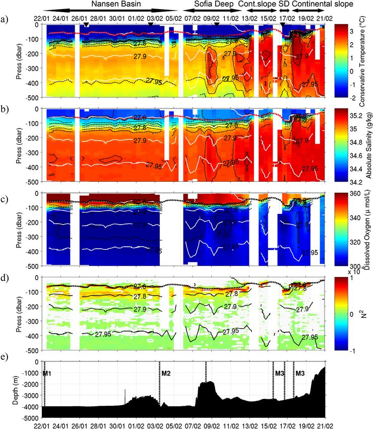
PUBLICATIONS
Journal of Geophysical Research: Oceans
RESEARCH ARTICLE                          Winter ocean-ice interactions under thin sea ice observed by
10.1002/2016JC012195
                                          IAOOS platforms during N-ICE2015: Salty surface mixed layer
Special Section:                          and active basal melt
Atmosphere-ice-ocean-
ecosystem Processes in a                     Koenig1, Christine Provost1, Nicolas Villacieros-Robineau1, Nathalie Senne
                                          Zoe                                                                          chael1, and
Thinner Arctic Sea Ice Regime:                         2
                                          Amelie Meyer
The Norwegian Young Sea ICE
Cruise 2015 (N-ICE2015)                   1
                                                                                      es, UPMC, Univ. Paris 6, CNRS-IRD-MNHN, Paris, France, 2Norwegian Polar
                                           Laboratoire LOCEAN-IPSL, Sorbonne Universit
                                          Institute, Fram Centre, Tromsø, Norway
Key Points:
 Large sea-ice melt over the inflowing
  Atlantic Water on the Svalbard          Abstract IAOOS (Ice Atmosphere Arctic Ocean Observing System) platforms, measuring physical param-
  northern continental slope in winter
 Sea-ice bottom melt associated with
                                          eters at the atmosphere-snow-ice-ocean interface deployed as part of the N-ICE2015 campaign, provide
  near-inertial waves and tides           new insights on winter conditions North of Svalbard. The three regions crossed during the drifts, the Nansen
 Winter hydrography shows a salty        Basin, the Sofia Deep, and the Svalbard northern continental slope featured distinct hydrographic properties
  mixed layer and three Atlantic Water
  pathways across and around the
                                          and ice-ocean exchanges. In the Nansen Basin, the quiescent warm layer was capped by a stepped halocline
  Yermak Plateau                          (60 and 110 m) and a deep thermocline (110 m). Ice was forming and the winter mixed layer salinity was
                                          larger by 0.1 g/kg than previously observed. Over the Svalbard continental slope, the Atlantic Water (AW)
Correspondence to:                        was very shallow (20 m from the surface) and extended offshore from the 500 m isobath by a distance of
Z. Koenig,                                about 70 km, sank along the slope (40 m from the surface) and probably shed eddies into the Sofia Deep. In
zklod@locean-ipsl.upmc.fr
                                          the Sofia Deep, relatively warm waters of Atlantic origin extended from 90 m downward. Resulting from
                                          different pathways, these waters had a wide range of hydrographic characteristics. Sea-ice melt was wide-
Citation:
Koenig, Z., C. Provost, N. Villacieros-
                                          spread over the Svalbard continental slope and ocean-to-ice heat fluxes reached values of 400 W m22
Robineau, N. Sennechael, and A. Meyer    (mean of 150 W m22 over the continental slope). Sea-ice melt events were associated with near 12 h fluc-
(2016), Winter ocean-ice interactions     tuations in the mixed-layer temperature and salinity corresponding to the periodicity of tides and near-
under thin sea ice observed by IAOOS
platforms during N-ICE2015: Salty
                                          inertial waves potentially generated by winter storms, large barotropic tides over steep topography, and/or
surface mixed layer and active basal      geostrophic adjustments.
melt, J. Geophys. Res. Oceans, 121,
7898–7916, doi:10.1002/
2016JC012195.

Received 28 JUL 2016                      1. Introduction
Accepted 1 OCT 2016
                                          With the rapid sea-ice decline [Comiso, 2012], the Arctic is the region in the world where climate change is
Accepted article online 5 OCT 2016
Published online 28 OCT 2016              most evident. The Arctic Ocean carries a large amount of ocean heat that has to be taken into account in the
                                          energy balance at the ice-ocean-atmosphere interface. Atlantic Water (AW) entering the Arctic Ocean through
                                          the Fram Strait with the West Spitsbergen Current (WSC) provides the main source of heat and salt to the Arc-
                                          tic Basin [Schauer et al., 2008; Aagaard et al., 1987]. The WSC splits into three branches upstream from the
                                          Yermak Plateau (Figure 1) [Quadfasel et al., 1987; Manley et al., 1992]: one branch recirculates back into the
                                          Fram Strait between 788N and 808N [Hattermann et al., 2016]; a narrow branch follows the western slope of
                                          the Yermak Plateau along the 1000 m isobath (called hereafter the Yermak Branch, YB) [Manley et al., 1992;
                                          Manley, 1995] and a main branch follows the northern continental slope of the Svalbard Archipelago along
                                          the 400–500 m isobath (called hereafter the Svalbard Branch, SB) [Sirevaag et al., 2011; Muench et al., 1992;
                                          Cokelet et al., 2008]. The Yermak Branch and the Svalbard Branch recombine east of the Yermak Plateau to
                                          continue as a boundary current eastward along the Eurasian continental slope [Rudels et al., 2015].
                                          A cold and fresh mixed layer lies above a strong pynocline and usually prevents the upwelling of AW up to
                                          the surface and hence sea-ice melt. This upper layer originates from low salinity shelf waters in most of the
                                          deep basins except in the Nansen Basin [Rudels, 2016]. In the Nansen Basin, as the warm AW inflow encoun-
                                          ters and melts sea ice, it creates an upper, low salinity surface layer that isolates the warm water from the
                                          sea ice and the atmosphere. The mixed layer in the Nansen Basin northeast of Svalbard forms as a result of
                                          AW cooling and freshening from sea-ice melt in the upper part of the water column. The AW heat released
C 2016. American Geophysical Union.
V                                         in the process is partly consumed by ice melt and partly escapes to the atmosphere. Evidence of basal sea-
All Rights Reserved.                      ice melt has been observed northeast of Svalbard in autumn [Steele and Morison, 1993] and on the Yermak

KOENIG ET AL.                                         WINTER OCEAN-ICE EXCHANGES N OF SVALBARD                                                            7898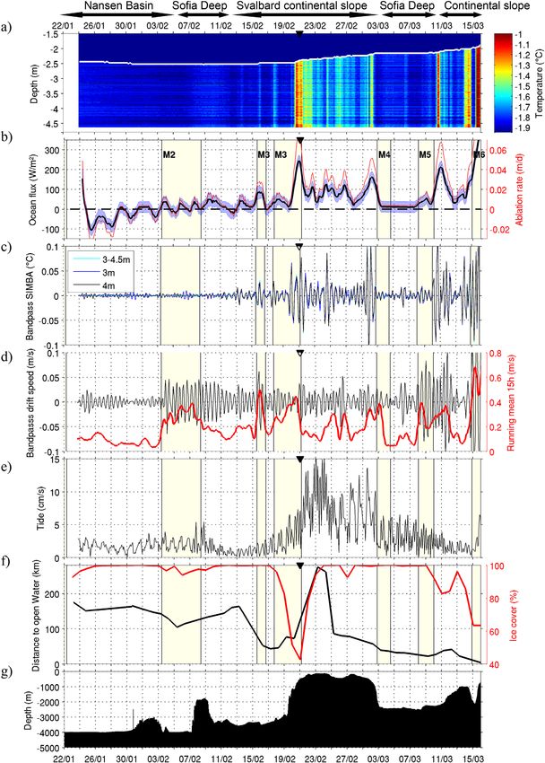
Journal of Geophysical Research: Oceans                                                                       10.1002/2016JC012195

                    Figure 1. Drift trajectory of the IAOOS platform during Floe 1 of N-ICE2015 campaign. Vertical colorbar is time. The Atlantic Water inflow
                    of the West Spitsbergen Current (WSC) splits into three branches, a recirculation to Fram Strait, the Yermak Branch (YB), and the Svalbard
                    Branch (SB) [Sirevaag et al., 2011]. The dashed line indicates the location of Floe 1 breakup when R/V Lance left and IAOOS7 continued
                    drifting alone. The two magenta lines show the offshore limit of the water originating from the Svalbard Branch over the Svalbard conti-
                    nental slope and the boundary between the Nansen Basin hydrography and the Sofia Deep hydrography, according to the data. Back-
                    ground is bathymetry (m). Yellow isolines are 0, 500, 700, 1000, 1500, and 2000 m. Bathymetry is from IBCAO (http://www.ngdc.noaa.gov/
                    mgg/bathymetry/arctic/arctic.html).

                    Plateau from late January to Mid-March 2003 [Mc Phee et al., 2003]. Winter sea-ice melt is also documented
                    by ice mass balance instrument during winter 2015 over the Svalbard Continental slope with ocean-to-ice
                    heat fluxes peaking at 400 W m22 (C. Provost et al., Observations of snow-ice formation in a thinner Arctic
                    sea ice regime during the N-ICE2015 campaign: Influence of basal ice melt and storms, submitted to Journal
                    of Geophysical Research, 2016). The trend in winter ice area loss North of Svalbard is close to 10% per decade
                    and the ice edge has retreated to the northeast along the AW pathway [Onarheim et al., 2014; Ivanov et al.,
                    2012]. Ivanov et al. [2016] suggest that the reemerging anomalies of ice free areas in midwinter Northeast
                    of Svalbard reveal a positive feedback with a ‘‘memory’’ of ice depleted conditions in summer transferring
                    to mid-winter via thinner ice more susceptible to lead formation allowing convection-induced upward heat
                    fluxes from the AW.
                    The Norwegian young sea ICE (N-ICE2015) expedition from January to June 2015 took place in this region
                    north of Svalbard to study ice-ocean-atmosphere interactions in a thinner Arctic sea-ice regime than it used
                    to be (Figure 1). This 6 month long campaign consisted of four drifting ice camps, relocated northward
                    each time the floes broke [Granskog et al., 2016]. The general hydrography and circulation patterns
                    observed during the 6-month drift are presented in Meyer et al. (A. Meyer et al., Winter to summer hydro-
                    graphic and current observations in the Arctic north of Svalbard, submitted to Journal of Geophysical
                    Research, 2016). Here we focus on mid-winter conditions as documented by IAOOS (Ice Atmosphere Arctic
                    Ocean Observing System) platforms deployed during Floe 1 of N-ICE2015 in January–February 2015 in the
                    middle of the polar night. These platforms carry an ice mass balance instrument monitoring temperature
                    across the air/snow/ice/ocean interface and an ocean profiler measuring conductivity hence salinity, tem-
                    perature and dissolved oxygen concentration down to 500 m or more. We use the IAOOS platform data to
                    examine the winter hydrography in the region and the ocean processes responsible for the winter basal
                    sea-ice melt over the Svalbard continental slope.
                    Section 2 presents the IAOOS platforms, the data processing and the platform drift over the western Nansen
                    Basin, the Sofia Deep and the Svalbard northern continental slope (Figure 1). Section 3 describes the distinct

KOENIG ET AL.                     WINTER OCEAN-ICE EXCHANGES N OF SVALBARD                                                                               7899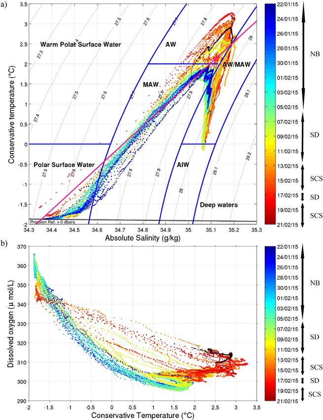
Journal of Geophysical Research: Oceans 10.1002/2016JC012195
hydrographic conditions sam-
pled by the profilers in the
three regions. Section 4 focuses
on the ocean-ice interface with
sea-ice growth and basal melt
processes. Finally in section 5
results are discussed and con-
clusions are drawn out.
2. IAOOS Platform and
Data
The IAOOS autonomous plat-
forms (Figure 2) document the
four media, ocean/ice/snow/
atmosphere, in the Arctic while
drifting with the ice [Provost
et al., 2015]. The atmospheric
part includes a GPS, a weather
mast and a microlidar [Mariage,
2015; Mariage et al., 2016]; the
ice/snow part an ice mass bal-
ance instrument [Jackson et al.,
2013]; and the ocean part an
ice-tethered profiler [Provost
et al., 2015] (Figure 2). Other
ice-tethered CTD profiling sys-
tems are used in the Arctic
[e.g., Krishfield et al., 2008;
Kikuchi et al., 2007]. Two plat-
forms were deployed during
Floe 1 (IAOOS7 on 22 January
and IAOOS8 on 26 January,
Table 1). Additional profiler
tests (IAOOS 9) were carried
out from 6 February to 19
February from a tent-covered
testing hole on Floe 1. The
three platforms were initially
located close to the ship, less
than 500 m from each other on
a second year ice floe, Floe 1.
R/V Lance drifted with Floe 1
from 15 January 15 (83.228N,
21.268E) until 21 February
(81.228N, 20.348E) when the
floe broke up (Figure 1). IAOOS
8 and 9 platforms were recov-
ered during Floe 1 breakup
while IAOOS 7 platform pur-
sued its drift until its recovery
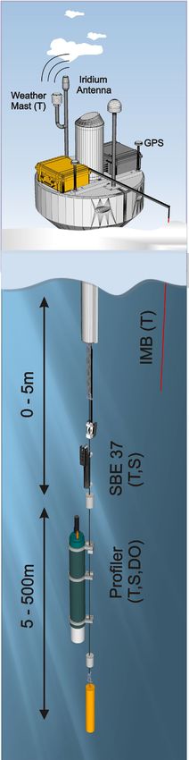
Figure 2. Schematic of the IAOOS platform showing weather mast, GPS, data transmission unit, by R/V Lance on March 16 (Fig-
ice mass balance unit (IMB measuring temperature through air, snow, ice, and upper ocean),
SBE37 instrument (recording temperature and salinity at 4 m depth) and the ocean profiler ure 1). The profiler on IAOOS 7
(measuring temperature, salinity, and dissolved oxygen concentration from 5 to 500 m depth). was lost on 21 February as the
KOENIG ET AL. WINTER OCEAN-ICE EXCHANGES N OF SVALBARD 7900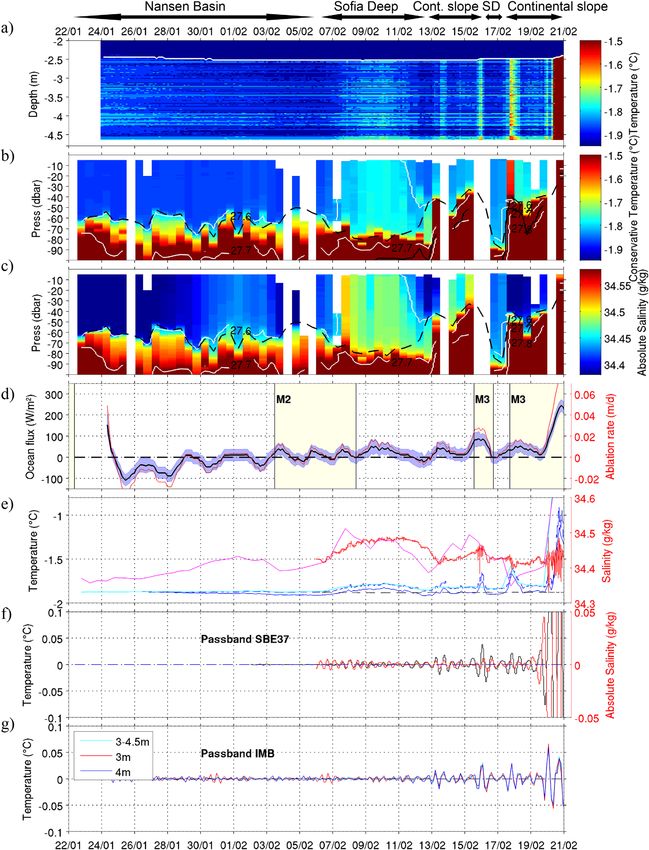
Journal of Geophysical Research: Oceans                                                     10.1002/2016JC012195

                                                                                             platforms drifted over ocean depths
                     Table 1. Characteristics of the IAOOS Platforms
                                                                                             smaller than 500 m (Table 1). Thus, from
                                               IAOOS 7             IAOOS 8      IAOOS 9
                                                                                             that date on, the only ocean data avail-
                     Deployment date         22 Jan 2015         26 Jan 2015   06 Feb 2015
                     Profiler lost            21 Feb 2015         21 Feb 2015
                                                                                             able are the near-ice ocean temperature
                     Recovery date           26 Mar 2015         23 Feb 2015   19 Feb 2015   profiles from the ice mass balance
                     Sampling rate (h)            12                  12            12       instrument.
                     Wire Length (m)             500                 500           850
                     SBE37                        No                 Yes           No The IAOOS weather mast provides local
                     IMB                         Yes                 Yes           No
                                                                                      atmospheric conditions. The ocean data
                     Good Profiles T               62                  50            26
                     Good Profiles S               53                  47            25collected from the IAOOS platforms doc-
                     Good Profiles DO              47                  44            21ument the warm water layer from the
                                                                                      Atlantic Water inflow, the halocline, the
                                                                                      mixed layer, the ocean-to-ice heat flux
                    and consequent winter basal ice melt (mid-January to mid-March 2015). The snow/ice mass balance instru-
                    ment data is analyzed in detail by Provost et al. (submitted manuscript) with a focus on snow-ice formation
                    observed in February and March 2015. Here we use the ice instrument data to examine closer the ocean-ice
                    interface.
                    The IAOOS weather mast recorded cold air temperatures below 2308C until 1 February and signatures of
                    the six main storms identified during N-ICE2015 by Hudson and Cohen [2015]: M1 (21–22 January), M2 (3–
                    8 February), M3 (15–21 February), M4 (3–4 March), M5 (8–10 March), and M6 (15–16 March) with air temper-
                    ature increase (up to 08C on 17 February) and large decrease in sea level pressure (down to 960 hPa on 9
                    March) (Figure 3a). M4 and M5 are recorded after Floe 1 breakup and the ship was not close to the IAOOS
                    platforms anymore. Hence, dates of M4 and M5 have been adjusted from Hudson and Cohen [2015] using
                    the data from the IAOOS weather mast. The GPS-derived platform drift speed increased during the storms
                    and reached 40 cm s21 during M2, 60 cm s21 on 16 February (M3), and even 100 cm s21 during M6
                    (Figure 3b).
                    The ice mass balance instrument from the Scottish Association for Marine Sciences (SAMS), hereafter called
                    SIMBA standing for SAMS ice mass balance for the Arctic, is composed of a thermistor chain of 5 m that pro-
                    vides profiles of temperature and a proxy of the thermal resistivity of the media with a 2 cm vertical resolu-
                    tion [Jackson et al., 2013]. The accuracy of each temperature sensor is 0.18C. SIMBA data from IAOOS 7 and
                    8 (SIMBA_2015h and SIMBA_2015i, respectively) have a 3 h sampling frequency. The SIMBA data analysis
                    that identifies the air/snow, snow/ice, and ice/ocean interfaces and estimates of heat flux densities is
                    detailed in Provost et al. (submitted manuscript). Here we use temperature data from SIMBA_2015h which
                    is the longest record with 51 days from 24 January to 16 March (Figure 3c). Snow thickness was 55 cm at
                    deployment and increased to 90 cm during storm M3 (Figure 3c). Ice thickness was 154 cm at deployment,
                    decreased to 125 cm on 9 March due to basal melt, and then increased to 145 cm from 9–11 March due to
                    snow-ice formation (Provost et al. submitted manuscript). The temperature time derivative (Figure 3d)
                    shows high-frequency variations in the atmosphere until storm M3 (there are no more sensors in the atmo-
                    sphere after M3 storm snow fall) that are dampened in the snow. In the ice the major changes in tempera-
                    ture are the cooling due to the initial refreezing of the deployment hole (until 1 February) and the
                    exothermal formation of snow-ice on 9 March. Changes in ocean temperature resulted in basal ice melt
                    that starts on 16 February.
                    The ocean profilers, from French manufacturer NKE (PROVOR SPI), a sliding profiler with inductive transmis-
                    sion, carried a Seabird SBE41CP CTD (Conductivity, Temperature, Depth) with an Aanderaa 4330 dissolved
                    oxygen (DO) optode. The profilers were set to perform two profiles a day from 500 m upward (850 m for
                    IAOOS9) starting at 6 am and 6 pm. They gathered a total of 138 profiles (62, 50, and 26 profiles for IAOOS7,
                    IAOOS8, and IAOOS 9, respectively; Table 1). The vertical resolution of the processed CTD data is 1 dbar in
                    the upper 400 dbars, 5 dbars from 400 to 550 dbars, and 10 dbars from 550 to 850 dbars; the vertical resolu-
                    tion in DO is 2 dbars over all depths. Salinity was calibrated and quality controlled using the ship CTD salini-
                    ty bottles (four dates) (Meyer et al., submitted manuscript). Following quality control, we retain all the
                    temperature profiles and remove 1% of the salinity profiles. Finally, the accuracy is estimated to be 0.0028C
                    in temperature, and 0.02 g/kg in salinity. Several profiles are missing or incomplete because of high drift
                    speeds (>0.4 m s21) impeding the ascent of the profiler. There were no bottle DO measurements available
                    during Floe 1 of N-ICE2015 to calibrate the DO data. DO accuracy is estimated comparing the deep values

KOENIG ET AL.                     WINTER OCEAN-ICE EXCHANGES N OF SVALBARD                                                      7901
Journal of Geophysical Research: Oceans                                                                                  10.1002/2016JC012195

Figure 3. Atmospheric and SIMBA data from 22 January to 16 March: (a) Sea level pressure and air temperature. Major storms are shaded in light yellow (M1, M2, . . .). (b) Drift velocity
estimated from GPS positions. (c) Temperature profiles from SIMBA (in 8C), white lines from Provost et al. [2016] indicate the air/snow/ice/ocean interfaces. (d) Time derivative of the
SIMBA temperatures (in 8C/d). The black triangle indicates the date after which there are no profiler data.

                                               of DO concentration (rather stable at 500m) between the three profilers. A difference of 3 lmol L21 is
                                               observed between IAOOS 8 and 9, and IAOOS 7. An offset of 3 lmol L21 is then applied to the oxygen data
                                               from IAOOS7 and the accuracy of the data is estimated to be at 3 lmol L21.
                                               IAOOS 8 also featured a Seabird SBE37 CTD recorder at about 4 m depth, sampling temperature, salinity,
                                               and pressure every 5 min from 22 January to 21 February. However, freezing of the SBE37 during deploy-
                                               ment prevents use of the temperature data before 27 January and of the salinity data before 6 February.
                                               The precision of the temperature sensor is 0.0028C and the conductivity sensor is 0.002 g/kg once converted
                                               in absolute salinity.
                                               In summary, the ocean data consist of temperature profiles in the upper 2 m with a 3 h time resolution
                                               from SIMBA-2015h (record length 51 days), temperature and salinity at 4 m depth with a 5 min resolution
                                               from the SBE37 (record length 25 days for temperature and 15 days for salinity), and temperature, salinity,
                                               and DO concentration with a 12 h resolution from 5 to 500 m from the profiler (record length 30 days). The

KOENIG ET AL.                                                WINTER OCEAN-ICE EXCHANGES N OF SVALBARD                                                                                7902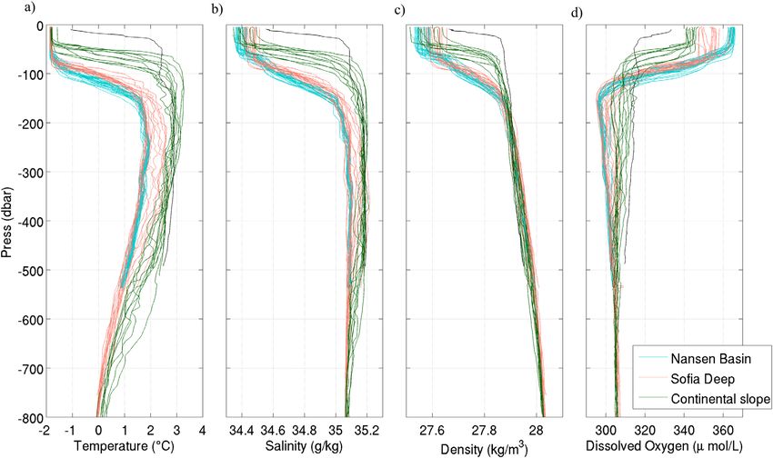
Journal of Geophysical Research: Oceans                                                 10.1002/2016JC012195

                    horizontal resolution depends upon drift velocity: for the profiler data it varies from 2 km on 2 February to
                    23 km on 15 February with an average of about 10 km.

                    3. Hydrography North of Svalbard in January–February 2015
                    The hydrographic sections presented in Figure 4 are composites of the three ocean profiler data. We use
                    the International Thermodynamic Equations of Seawater (TEOS-10) framework [McDougall et al., 2012] with
                    conservative temperature CT (8C) and absolute salinity SA (g/kg). In the region, absolute salinity values
                    exceed practical salinity values by about 0.16. We follow water mass definitions from Rudels et al. [2000, Fig-
                    ure 2] (Figure 5a) adapted to absolute salinity and conservative temperature. The warm layer comprises two
                    main water types: Modified Atlantic Water (MAW) (temperatures between 0 and 28C) and Atlantic Water
                    (AW) (temperatures larger than 28C). DO concentration varies from low values (290–310 lmol L21) in the
                    warm layer to larger values in the upper layer (range 340–367 lmol L21) (Figure 4c). The surface layer shows
                    absolute salinities between 34.35 and 34.55 g/kg, corresponding to practical salinities of 34.19 and 34.39
                    psu, respectively, slightly larger than those observed previously in the region (e.g., 34.1–34.2 psu) [Kikuchi
                    et al., 2004; Rudels et al., 2000; Sirevaag and Fer, 2009]. Near-surface temperatures are often at the freezing
                    point or close to it. The three regions crossed by Floe 1 drift, the Nansen Basin from 22 January to 6 Febru-
                    ary, the Sofia Deep and the tip of the Yermak Plateau from 6 to 12 February and on 17 February (called
                    hereafter Sofia Deep) and the Svalbard continental slope the rest of the time, present clearly distinct charac-
                    teristics in the warm water layer and in the surface layer (Figures 1 and 4).

                    3.1. The Warm Water Layer From the Atlantic Ocean
                    The warm water layer (with temperatures larger than 08C) extends from around 100 m to deeper than
                    500 m (Figure 4a), the deep 08C isotherm is at about 800 m in the 850 m deep IAOOS 9 profiles (Figures 6a
                    and 7a).
                    In the Nansen Basin (depth > 4000 m), the warm water, composed of MAW, shows layering with two cores
                    (at depths of around 250 and 400 m) with the same temperatures (around 11.88C), different salinities
                    (35.08 and 35.12 g/kg), and thus densities of 27.91 and 27.95, respectively (Figure 5a). The constant depth
                    of the two cores is highlighted in the Brunt V€ais€al€a frequency panel (Figure 4d). DO concentration is around
                    305 lmol L21 in the MAW (Figures 4d and 5b). Hydrographic properties of Nansen Basin profiles (in blue in
                    Figure 6) show little scatter in the AW range below 150 m. Isopycnals remain at the same depth except for
                    significant isopycnal displacements at depth (80 m displacement at 400 m) after 3 February coincident with
                    storm M2.
                    Over the continental slope off Svalbard, roughly from 12 February onward, the warm water is AW with a sin-
                    gle shallower core (150 m), warmer temperature (>2.58C), higher salinity (>35.15 g/kg), and slightly larger
                    DO concentration (315 lmol L21) (Figure 5). This AW appears to come directly from Fram Strait (Figure 1)
                    [Sirevaag and Fer, 2009]. The last profile (21 February) on the slope over 600 m shows AW as close as 20 m
                    from the surface (black profile in Figures 5b and 6). It is the warmest profile below 300 m (2.98C), and among
                    the saltiest and the lowest in DO concentration (35.19 g/kg, 312 lmol L21). The peculiar upper structure of
                    the profile is examined more closely in section 3.2. Profiles over the Svalbard Continental Slope show an off-
                    shore deepening of the top of the AW layer (08C isotherm) and a scatter of hydrographic properties at
                    depth indicative of lateral mixing. On 17 February, as the platform drifted to the north, the profiler sampled
                    MAW from the Sofia Deep at 81.88N and 18.58E–198E. This provides a local offshore limit of the location of
                    the Atlantic Water coming from the Svalbard Branch (Figure 1, magenta line and Figure 7).
                    Between 6 and 12 February, the profiler measured water over the northern tip of the Yermak Plateau and
                    over the Sofia Deep (Figures 1 and 4). The warm layer shows variations in isopycnal depths with amplitudes
                    of about 100 m at 400 m decreasing toward the surface to values of 80 m at 200 m, and 10 m at 100 m. The
                    troughs in isopycnal depth observed on 7 February likely correspond to topographically induced upwelling
                    of deep fresher water that mixes with AW (Figure 7) (see section 5). Apart from these upwelling events, the
                    warm layer comprises water from the Nansen Basin (Figure 4, 10–11 February). During 8 February and 11–
                    12, the layer contains water warmer and saltier than in the Nansen Basin associated with isopycnal ridges.
                    The warm water on 8 February at about 82.28N located on the slope of the Yermak Plateau (depth around
                    1800 m) is probably the Yermak Branch, with an AW core at 300 m, propagating southward from the tip of

KOENIG ET AL.                  WINTER OCEAN-ICE EXCHANGES N OF SVALBARD                                                       7903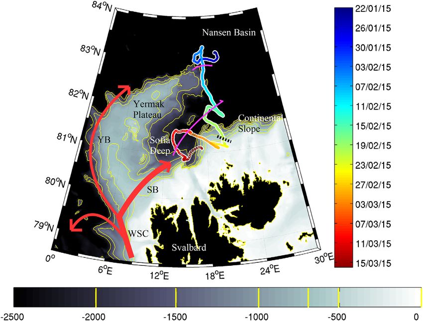
Journal of Geophysical Research: Oceans                                                                                     10.1002/2016JC012195

Figure 4. Composite section from the 3 profiler data (12 h averaged) of (a) conservative temperature (8C). The thick black line is the 08C isotherm. (b) Absolute salinity (g/kg). (c) Dis-
solved oxygen concentration (lmol L21). Thin black dashed lines are, respectively, temperature, salinity, and dissolved oxygen concentration isolines. Thin white lines are isopycnals. (d)
Brunt V€ais€al€a frequency (N2) along the drift (1024 s21). The thin black lines are isopycnals. (e) Bathymetry along the drift trajectory. Dashed lines delimit storms. Thick dashed lines (red
or black) are the mixed layer depth. Dates when the ship CTD were used to calibrate salinity data appear as black triangles. Arrows on the top indicate the ‘‘hydrographic regions’’ of
Nansen Basin, Sofia Deep (SD), and Svalbard continental slope. Missing profiles are white.

KOENIG ET AL.                                                  WINTER OCEAN-ICE EXCHANGES N OF SVALBARD                                                                                   7904
Journal of Geophysical Research: Oceans 10.1002/2016JC012195
Figure 5. (a) Conservative temperature-absolute salinity diagram from the IAOOS profiler data. Water mass boundaries are from Rudels
et al. [2000]: Atlantic Water (AW), Modified Atlantic Water (MAW), and Atlantic Intermediate Water (AIW). (b) Conservative temperature-DO
concentration diagram. Colorbar is time and corresponding hydrographic provinces, Svalbard continental slope (SCS), Sofia Deep (SD), and
Nansen Basin (NB), crossed during the drift are indicated. The black profile in both diagrams corresponds to the last one (20 February after-
noon) over very shallow waters. The magenta line is the mixing line in the Nansen Basin between Polar Surface Water and Modified
Atlantic Water. The blue dots under the magenta line in Figure 5a draw the shape of the convective halocline.
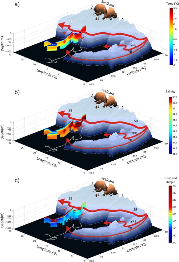
the Yermak Plateau (82.88N, 168E) following the 1000–2000 m isobath (Figures 1, 4, and 7). The warm water
on 11–12 February (82.28N, 198E) with a core at 300 m may originate from a branch flowing through the Yer-
mak Pass (a 700 m deep passage through the Yermak Plateau at 818N) [Gascard et al., 1995, Figure 34] or
could be a deep eddy that detached from the Svalbard Branch and sank (Figure 7). There is not enough
data to draw further conclusions. As a result of these different processes or paths, the range of hydrographic
characteristics in the warm water layer is larger in the Sofia Deep profiles (red in Figure 6) than in the
KOENIG ET AL. WINTER OCEAN-ICE EXCHANGES N OF SVALBARD 7905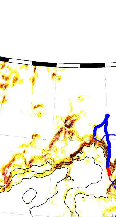
Journal of Geophysical Research: Oceans                                                                                    10.1002/2016JC012195

Figure 6. Vertical profiles from the profilers of (a) conservative temperature (8C), (b) absolute salinity (g/kg), (c) density (kg m23), and (d) dissolved oxygen concentration (lmol L21). Blue
profiles are from the Nansen Basin, red profiles from the Sofia Deep and green profiles from the Svalbard continental slope. Black profiles correspond to the last profile of the drift (20
February afternoon) over very shallow waters.

                                               Nansen Basin (blue in Figure 6) or the Svalbard continental slope profiles (green in Figure 6). In particular,
                                               the lowest salinity observed on 7 February where 35.05 g/kg at 300 m depth (Figure 6b), and the largest
                                               salinity at 370 m were 35.21 g/kg on 12 February (Figures 5a and 6b).
                                               The AW is DO-enriched (from 300 to 315 lmol L21) compared to the MAW (295–305 lmol L21) indicating
                                               that warm waters from the Svalbard Branch have been in contact with the atmosphere more recently than
                                               waters from the Nansen Basin (Figures 4c and 5b). The Nansen Basin (MAW) profiles show a DO-minimum
                                               ( 300 lmol L21) at about 140–150 m at the base of the lower halocline (blue in Figure 6d) whereas the
                                               shallowest Svalbard Branch (AW) profile (black in Figure 6d) is homogeneous below 20 m with DO values
                                               of 310 lmol L21. The spread in DO concentration in the other profiles is indicative of vertical mixing
                                               (Figure 6d).

                                               3.2. The Upper Layer Characteristics
                                               Over the Svalbard continental slope and the Sofia Deep, the depths of the thermocline, the halocline, and
                                               the pycnocline coincide. Gradients are steeper and shallower (40 m) above the Svalbard Branch, while
                                               weaker and deeper (90 m) over the Sofia Deep (Figure 6). Over the Nansen Basin, the thermocline is cen-
                                               tered at 110 m whereas the halocline (pycnocline) comprises an upper halocline (upper pycnocline) cen-
                                               tered at 60 m and a lower halocline (lower pycnocline) centered at 110 m (Figure 6). The processes
                                               responsible for this double pycnocline structure potentially involve formation of a convective cold halocline
                                               as ice is formed and/or the advection of cold salty water from shelves [e.g., Rudels et al., 1996; Kikuchi et al.,
                                               2004]. The observed T-S curves from the Nansen Basin fall below the mixing line joining T-S values at 220
                                               and 140 m (magenta line in Figure 5) and form a bend separating low salinity freezing surface layers from
                                               the thermocline waters. Indeed, the lower halocline water and the top of the thermocline water have salini-
                                               ty larger (temperature lower) than the mixing line between the AW and the Polar Surface Water. This fea-
                                               ture in the T-S diagram in the Nansen Basin indicates a convective mechanism leading to a stepped
                                               halocline after summer melt and refreezing [Kikuchi et al., 2004, Figure 4].

KOENIG ET AL.                                                 WINTER OCEAN-ICE EXCHANGES N OF SVALBARD                                                                                 7906
Journal of Geophysical Research: Oceans 10.1002/2016JC012195 Figure 7. Three-dimensional plot of (a) conservative temperature (8C), (b) absolute salinity (g/kg), and (c) dissolved-oxygen concentration (lmol L21). Isolines are 500, 700, 1000, and 1500 m. Red full arrows describe paths for the warm Water Inflow: the Yermak Branch (YB), the Svalbard Branch (SB), and the Yermak Pass branch (YPB) [Sirevaag et al., 2011; Rudels et al., 2000]. Dashed red lines are indication of downwelling of the Atlantic Water down the continental slope into the Sofia Deep. KOENIG ET AL. WINTER OCEAN-ICE EXCHANGES N OF SVALBARD 7907
Journal of Geophysical Research: Oceans                                                 10.1002/2016JC012195

                    The last profile on the slope with near-surface Atlantic Water at 20 m measures the warmest and among
                    the saltiest waters below 300 m and shows a stepped structure in both temperature and salinity, with a gra-
                    dient at 130 m, compensated in density (black profile in Figures 5 and 6). Below 30 m depth, stratification is
                    very weak (Figures 4d and 6c) and temperature and salinity profiles are well mixed on each side of the step
                    (Figures 6a and 6b). This structure suggests the loss of heat in the upper 120 m laterally and vertically along
                    the Svalbard Branch, followed by the advection of a layer of fresher melt water on top of it or active ice
                    melt creating a sharp near-surface thermocline and halocline [Rudels, 2016].
                    Apart from this peculiar profile, on the slope, the mixed layer depth (MLD) (here defined as the depth where
                    density is larger than the density at 10 m by 0.03 kg m23) is on average 40 m in the Svalbard Branch, 90 m
                    in the Sofia deep, and 60 m in the Nansen Basin. Note that the MLD is quite insensitive to the precise criteri-
                    on as the pycnocline is sharp [e.g., Timmermans et al., 2012; Toole et al., 2010]. The surface mixed layer is
                    cold (21.88C, the freezing temperature), with low salinity (34.35–34.50 g/kg) and DO-enriched compared
                    to the MAW/AW (340–370 lmol L21). The DO-enriched mixed layer corresponds to Polar Surface Water
                    (Figure 5). The salinity range is quite large from 34.35 to 34.51 g/kg and even reaching 34.55 g/kg for the
                    last profile (Figure 6b). These salinity values are high compared to MIMOC climatological values, 10.25 g/kg
                    (Meyer et al., submitted manuscript).
                    The Brunt-V€ais€al€a frequency [Gill, 1982] is larger above the Svalbard continental slope as the warm waters
                    are denser in the AW than in the MAW (Figure 4d). The main pynocline reaches Brunt-V€ais€al€a frequency val-
                    ues larger than 2 3 1024 s21 (Figure 4d), of the same order as in Fer [2009]. The deeper thermocline and
                    lower halocline in the Nansen Basin show large Brunt-V€ais€al€a frequency (5 3 1025 s21) under the main
                    pycnocline.
                    The mixed layer DO concentration is larger in the Nansen Basin than over the Svalbard Branch (360 lmol
                    L21 and 345 lmol L21, respectively, Figures 4c and 5b). This may be an indication of oxygen consumption
                    and hence of biomass remineralization over the AW that does not occur in the mixed layer over the MAW. It
                    may also be due to upwelling of low DO concentration AW through the pynocline over the Svalbard Branch
                    that does not occur in the Nansen Basin.

                    4. Upper Ocean, Sea-Ice Formation and Basal Melt
                    We now focus on the ice-ocean interface in two steps, first analyzing and comparing the SIMBA, SBE37, and
                    profiler data until 21 February, and then second by analyzing the only data available after 21 February
                    which is the SIMBA temperature data.

                    4.1. Upper Ocean Until the Loss of the Profilers (21 February)
                    4.1.1. Consistency Between the Instruments in the Vertical
                    Temperature time series from the upper 2 m of the ocean from SIMBA (3 h resolution shown with an
                    adapted colorbar to focus on the ice-ocean interface, Figure 8a) are consistent with the temperature time
                    series at 4 m from the SBE37 (5 min sampling) (Figure 8e) and the temperature time series in the upper
                    30 m from the profiler (12 h sampling) (Figure 8b). Several events with under-ice temperatures above freez-
                    ing temperature are identified.
                    The temperature increase observed from 7 to 11 February in the SIMBA, SBE37, and upper-ocean profiler
                    data (T  21.758C; Figures 8a and 8b, Figure 8e) coincides with an increase in salinity measured by the
                    SBE37 (S  34.35–34.5 g/kg) and the ocean profiler (S  34.48 g/kg; Figures 8e and 8c).
                    On 16, 18, and 20 February (Figure 8a), the under-ice temperature is above freezing (about 0.158C, 0.28C,
                    and 1.88C, respectively). The 18 and 20 February events are associated with warmer water down to the halo-
                    cline (profiler data; T  21.558C and T  218C, respectively) (Figure 8b). There is no profiler data on 16 Feb-
                    ruary. These three warm events occur over the Svalbard Branch, where the 08C isotherm is shallow
                    (between 60 and 18 m, Figure 8c).
                    From 30 January to 3 February, profiler data (below 8 m) indicate a salinity increase in the mixed layer
                    (34.45 g/kg instead of 34.4 g/kg, Figure 8c), while temperature remains stable (around 21.858C, Figure
                    8b). There is no signal in temperature in the upper 4 m of the ocean (SIMBA or SBE37) (Figures 8a and 8e).
                    This salinity-only event happens before M2, when the platform is located on the edge of the slope of the

KOENIG ET AL.                  WINTER OCEAN-ICE EXCHANGES N OF SVALBARD                                                       7908
Journal of Geophysical Research: Oceans 10.1002/2016JC012195 Figure 8. (a) SIMBA temperature zoomed on the ocean (scale 228C; 21.58C). (b) Conservative temperature (8C) in the upper 100 m from the profilers. The full black line is the 08C isotherm. (c) Absolute salinity (g/kg) in the upper 100 m from the profilers. White lines are isopycnals. The thick dashed line is the mixed layer depth. Missing data points are white. (d) Ocean Flux (left axis, W m22) and ablation rate (right axis, m/d), at the ice/ocean interface deduced from SIMBA data [Provost et al., 2016]. Blue shaded area is the ocean heat flux uncertainty [Provost et al., 2016]. Storm periods are shaded in light yellow. (e) Left axis: temperature from SIMBA (mean of the upper 2 m, 3 h sampling, blue), from SBE37 (4 m, 5 min sampling, dashed blue) and from profilers at 20 m (12 h sampling, cyan). The dotted line is the freezing temperature. Right axis: Salinity from SBE37 (red) and from profilers at 20 m (magenta). (f) Data from SBE37 filtered between 8 and 16 h: temperature (left axis, black), salinity (right axis, red). (g) Band-pass filter between 8 and 16 h of SIMBA temperatures at 3 m (red), 4 m (blue), and averaged between 3 and 4.5 m (black). KOENIG ET AL. WINTER OCEAN-ICE EXCHANGES N OF SVALBARD 7909
Journal of Geophysical Research: Oceans                                                   10.1002/2016JC012195

                    Yermak Plateau (seafloor depth about 3000 m). A salty mixed layer is characteristic of the Yermak Plateau
                    (Meyer et al., submitted manuscript).
                    The ocean (SIMBA, profilers and SBE37) data, therefore, provide a consistent picture of the upper-ocean vertical
                    structure despite the difference in time resolution (3 h for the SIMBA, 12 h for the profiler and 5 min for the
                    SBE37). For the following, it is important to recall that in the Nansen Basin the thermocline located at about
                    90 m depth is deeper than the pycnocline/halocline (around 60 m), while in the Sofia Deep and Svalbard
                    Branch the three gradients coincide and are shallower than 60 m, around 40 m. The ocean heat flux (Figure 8d)
                    was estimated as the sum of the latent heat flux (calculated from the time evolution of the ice-ocean interface
                    depth) and the conductive flux in the ice next to the ocean interface (calculated from the vertical derivative of
                    temperature) (Provost et al., submitted manuscript). The negative fluxes at the beginning of the time series
                    until 26 January (Figure 3d) correspond to lateral fluxes associated with the refreezing of the deployment hole
                    of the SIMBA. From 26 January to 1 February, sea-ice formation (growth) most likely caused the negative fluxes
                    in accordance with the formation of the stepped halocline in the Nansen Basin. The ocean flux is significantly
                    positive on several occasions, 9–11 February (50 W m22), 16 February (100 W m22), and 20 February (250 W
                    m22), when the near-ice ocean temperature is above freezing and coincide with sea-ice basal melt.
                    We now focus on the high frequencies observed in the under-ice ocean data (SIMBA and SBE37). The daily
                    resolution of the profiler data is not sufficient to examine the around 12 h period typical of tides and near-
                    inertial internal gravity waves in the area.
                    4.1.2. High-Frequency Variations in Temperature and Salinity
                    The melting events, associated with ocean temperature peaks, also correspond to large high-frequency fluc-
                    tuations detected in the 5 min sampling SBE37 data (Figure 8e). These high frequencies in salinity and tem-
                    perature, retrieved when subtracting a 15 min running mean, have amplitudes up to 0.05 g/kg and 0.038C
                    and are largely anticorrelated (r 5 20.88). These melt-associated high-frequency signatures could result
                    from vertical mixing and overturning induced by salt releases from warming sea ice [Widell et al., 2006].
                    Variations with a close to 12 h period are conspicuous in certain parts of the SBE37 salinity time series (Figure
                    8f). They are less clear in the temperature time series because of the large temperature scale adapted to the
                    large temperature range in Figure 8e. The close to 12 h period corresponds to the period of both semidiurnal
                    tides and near-inertial internal waves generated in the upper ocean around 828N, by passing storms or by geo-
                    strophic adjustment of strong mesoscale structures [Dosser et al., 2014]. Temperature and salinity variations in
                    the 8–16 h bandwidth were extracted from the SBE37 data (Figure 8f). Salinity fluctuation amplitudes are below
                    0.006 g/kg most of the time except during the large melt events after 19 February where amplitudes larger than
                    0.05 g/kg are observed. Temperature fluctuations in this period range exceed 0.018C for each melt event and
                    even 0.358C for the last event. This amplitude of 0.358C corresponds approximately to an isotherm displacement
                    of 15 m according to the last temperature profile (20 February 18:00: 21.158C at 6 m and 20.708C at 14 m).
                    In conclusion, the basal melt events until 21 February are associated with warming of the entire mixed layer
                    when heat comes from the AW of the Svalbard Branch to the surface. Possible processes for the heat trans-
                    fer from AW to the surface are discussed in section 4.2.
                    As observed in Fig. 3, basal melt is very active after February 21, when the only available data are that from
                    SIMBA. SIMBA sensors do not have the accuracy of a SBE37 sensor and the sampling frequency was 3 h
                    instead of 5 min. We cannot examine very high frequencies with the SIMBA data, however, we now show
                    that we can get reliable information about the close to 12 h fluctuations. We produced three temperature
                    time series out of the SIMBA profiles: two time series of the temperature averaged over 10 sensors around 3
                    and 4 m depth, and one time series of the temperature averaged over 75 sensors between 3 and 4.5 m. We
                    applied an 8–16 h band-pass filter to the three temperature time series (Figure 8g). The three times series
                    provide near 12 h fluctuations that are consistent with those extracted from the SBE37 data although with
                    somewhat reduced amplitudes: variations near the 12 h period are observed during the melting events on
                    13, 16, and 20 February with similar amplitudes to those derived from the SBE37 during the first two small
                    events and smaller amplitude on 20 February (Figure 8g). We now examine the full SIMBA time series.

                    4.2. Basal Ice-Melt Documented by SIMBA Data Until 15 March
                    Sea-ice melt is observed from 15 February to 2 March over the warm mixed layer of the Svalbard continen-
                    tal slope and estimated ocean to ice flux has a mean value of 100 W m22 over those 2 weeks (Figures 9a

KOENIG ET AL.                  WINTER OCEAN-ICE EXCHANGES N OF SVALBARD                                                         7910
Journal of Geophysical Research: Oceans 10.1002/2016JC012195 Figure 9. (a) SIMBA temperature zoomed on ocean from 22 January to 16 March. (b) Ocean flux (left axis, W m22) and ablation rate (right axis, m/d), at the ice/ocean interface deduced from the SIMBA data. Blue shaded area is the ocean heat flux uncertainty [Provost et al., 2016]. The black triangle is the date after which there are no profiler data. (c) SIMBA temperature band-pass filtered between 8 and 16 h at 3 m (red), 4 m (blue) and averaged between 3 and 4.5 m (black). (d) Drift speed of IAOOS7 platform band-pass filtered between 8 and 16 h (left axis) and filtered using a 15 h running mean (right axis). (e) Tide velocity (m/s) from the AOTIM5 model [Padman and Erofeeva, 2004] colocated with the IAOOS7 platform drift. (f) Distance of SIMBA-2015h to open water (left axis) from Itkin et al. [2016] and colocated ice cover (%) from AMSR-2 (right axis). (g) Bathymetry along the track. Storm periods are shaded in light yellow. KOENIG ET AL. WINTER OCEAN-ICE EXCHANGES N OF SVALBARD 7911
Journal of Geophysical Research: Oceans                                                   10.1002/2016JC012195

                    and 9b). On 3 March, SIMBA drifts away from the continental slope (Figures 1 and 9d) and sea-ice melt stops
                    as the under-ice water is at freezing temperature (21.88C, Figure 9a). Sea-ice melt resumes on 11 March, as
                    the platforms drifts back over the continental slope and the shallow Svalbard Branch. A maximum sea-ice
                    melt is observed at the end of the time series (15 March) as the platforms drifts southward over warm
                    waters (around 218C). The estimated heat flux then exceeds 350 W m22 (Figure 9b). In 1 month, the SIMBA
                    witnessed 71 cm of sea-ice basal melt.
                    In the SIMBA under-ice temperatures, large fluctuations with periodicities around 12 h and amplitudes
                    reaching 0.18C are observed and coincide with basal sea-ice melt (19 February to 2 March and 10–16 March)
                    (Figures 9c and 9a). These large 12 h period fluctuations occur over rough topography (Figure 9g) and/or
                    after large storms M5 and M6 (Figure 9c).
                    A variety of energy sources can generate near-inertial internal gravity waves with fluctuations close to 12 h,
                    including atmospheric forcing [Fer, 2014], tides interacting over topography and geostrophic adjustment of
                    mesoscale features [Alford et al., 2016]. Amplitudes of near-surface temperature variations at the near-inertial
                    wave frequency estimated from the SIMBA observations (Figure 9c) were compared to ice drift speeds (Figure
                    9d), barotropic tide velocity amplitudes (estimated using AOTIM-5 model outputs, Padman and Erofeeva
                    [2004] as in Meyer et al., (submitted manuscript)) (Figure 9e), sea-ice concentration from AMSR2 (https://earth-
                    data.nasa.gov), distance to ice edge (P. Itkin et al., Sea ice deformation from the buoy array: Identification of
                    deformation events and comparison to other datasets (SEDNA, FRAMZY, atmosphere), submitted to Journal of
                    Geophysical Research, 2016, Figure 9f), and seafloor roughness (Figure 9g) to get some insight into the mecha-
                    nisms responsible for those 12 h near-surface temperature variations. Ice drift speed was decomposed into
                    inertial ice speed using the same 8-16 h band pass filter and subinertial low frequency ice speed (Figure 9d).
                    Large amplitudes in inertial ice drift velocities are observed during and just after M3, and the ice pack concen-
                    tration falls to 40% (Figures 9d and 9f). The presence of leads and open water (lower ice concentration) and
                    the proximity to the ice edge (Figure 9f) allow more direct transfer of energy from the atmosphere to the
                    ocean, as observed during the second part of M3 and during M5 and M6 (Figure 9c). The fluctuations in tem-
                    perature with amplitude larger than 0.18C could be storm-induced inertial waves. They are generated over
                    ice-free ocean and detected when the platform is near open waters (ice edge or leads). The 12 h fluctuation
                    signature in under-ice temperature is modulated by the depth of the thermocline: when the thermocline is
                    below the pycnocline as in the Nansen Basin there is no signature of inertial waves in under-ice temperature.
                    The large episodic 12 h temperature fluctuations from 21 February to 3 March are concomitant with large
                    tides over shallow topography at a time when the ice edge is distant by over 200 km and sea-ice concentra-
                    tion is close to 100%. The barotropic tide interacting with the shallow bottom topography could induce
                    near-inertial waves with the observed under-ice temperature signal. As described in Rippeth et al. [2015],
                    large bathymetry gradients associated with large barotropic tides can cause enhanced vertical heat flux
                    from the AW across the pynocline through near-inertial waves development.
                    Geostrophic adjustment of mesoscale features can also generate near-inertial waves [Alford et al., 2016]. The
                    largest 12 h under-ice temperature signal is observed over the maximum of gradient of the continental
                    shelf (21 February, 3, 11, and 15 March, Figures 9g and 10), which corresponds with the offshore boundary
                    of the Svalbard Branch (Figure 1).
                    The precise mechanisms that could have generated the near-inertial waves in the area are difficult to assess
                    as tides, rough topography, and fronts are often concomitant when near-inertial wave signatures are
                    recorded in the SIMBA and SBE37 data. Furthermore an internal wavefield is composed of both locally and
                    remotely generated waves. The data do not permit to distinguish between locally generated downward
                    propagating waves and remotely generated upward propagating waves. However, it seems that the wind
                    has a major influence at the end of the time series when the platforms are in less compact ice, near leads or
                    the ice edge, and that the tidal effects dominate from 10 February to 3 March.

                    5. Summary and Discussion
                    The deployment of IAOOS platforms during the N-ICE2015 campaign [Granskog et al., 2016] provided new
                    insights on winter conditions in an area historically poorly sampled during that season (Meyer et al., submit-
                    ted manuscript).

KOENIG ET AL.                  WINTER OCEAN-ICE EXCHANGES N OF SVALBARD                                                        7912
Journal of Geophysical Research: Oceans 10.1002/2016JC012195
Figure 10. Summary of the study. Background is the bathymetry gradient amplitude (without units). Black contours are 0, 500, 700, 1000, 1500, and 2000 m depths. The drift trajectory is
red when Floe 1 drifted over Atlantic Waters, and blue when Floe 1 drifted over the Modified Atlantic Waters. The trajectory is thick during storms and thin otherwise. The black dashed
line (around 81.28N, 208E) in the map indicates the location of Floe 1 breakup when R/V Lance left and IAOOS7 continued drifting alone. The gray plots describe the ice-ocean interface
and the warm water layer at several key locations. The dashed line in the panel separate comments on the surface (top part) and on the deep warm waters (bottom part).
The three regions crossed by Floe 1, the Nansen Basin, the Sofia Deep, and the Svalbard continental slope
(Figures 7 and 10) presented distinct hydrographic conditions and ice-ocean interactions.
1. In the Nansen Basin the warm layer was deep, quiescent with layering in agreement with a description
by Rudels et al. [2000] and capped by a stepped halocline due to local ice formation after summer melt
as described in Kikuchi et al. [2004]. Ice was forming in the Nansen Basin as SIMBA-derived ocean-to-ice
fluxes were negative and the upper layer salinity was larger than previously observed by 0.1 g/kg. A pos-
sible explanation for this larger salinity is that, in an Arctic region with thinner ice and leads, new-ice
would grow faster in winter and salt release would be more important [Ivanov et al., 2016].
2. Over the Svalbard continental slope, the warm AW from the Svalbard Branch was only 20–40 m from the
sea surface. Profiler observations documented an 70 km AW extension offshore the 500 m isobath and
an offshore deepening of the AW over the continental slope. They were supportive of offshore AW eddy
KOENIG ET AL. WINTER OCEAN-ICE EXCHANGES N OF SVALBARD 7913Journal of Geophysical Research: Oceans 10.1002/2016JC012195
shedding as recently documented further east (308E) with velocity observations by Våge et al. [2016]. The
lateral extension and mesoscale activity may be only winter features as the Atlantic Water inflow is sea-
sonally variable with a larger transport in winter [Hattermann et al., 2016] (Z. Koenig et al., Atlantic Waters
inflow north of Svalbard: insights from IAOOS observations and Mercator Ocean global operational sys-
tem during N-ICE2015, submitted to Journal of Geophysical Research, 2016). SIMBA documented very
large ocean surface temperature on the shelf and large sea-ice basal melt. Mixed layer temperatures
were large because of enhanced local vertical heat fluxes from AW possibly due to: tides, mesoscale fea-
tures, vertical convection during overturning events, steep bathymetry, or wind forcing near the ice edge
and over leads.
3. In the Sofia Deep, the range of warm water characteristics was large and suggested different processes
and water paths (Figures 7 and 10): upwelling of deep fresher water into the AW layer as possibly linked
to tidal activity over rough topography [Luneva et al., 2015], mesoscale structures with AW cores from
the Yermak Branch, the Svalbard Branch, or coming from the Yermak Pass (a passage through the Yer-
mak Plateau deeper than 700 m at 818N) [Gascard et al., 1995; Rudels et al., 2000] (Figure 7). High-
resolution operational model outputs analyzed in a companion paper (Koenig et al., submitted manu-
script) support these interpretations in terms of warm water paths and eddy activity.
The mixed layer was at the freezing temperature except above the Yermak Plateau slope and above the
Svalbard Branch (Figure 10). The salty surface mixed layer located on the deep edge of the Yermak Plateau
probably originates from the Yermak Plateau (Meyer et al., submitted manuscript). Operational model out-
puts confirm the difference in salinity between the salty Yermak Plateau and the fresh Nansen Basin mixed
layers in winter (Koenig et al., submitted manuscript). The under-ice temperature, slightly above freezing
over the deep slope of the Yermak Plateau, did not generate significant melt. In contrast, the thin and warm
mixed layer above the Svalbard continental slope resulted in significant sea-ice melt in the middle of winter
(Figure 10). The warming of the under-ice ocean is clearly visible in the SIMBA data. Near-inertial fluctua-
tions in the under-ice temperature records suggest that near-inertial gravity waves bring heat from the shal-
low AW inflow up to the surface. However, the deep expression of the near-inertial signal could not be
examined with the 12 h sampling of the IAOOS profiler during N-ICE2015. A higher sampling rate should be
used in the future to enable studies like those by Dosser et al. [2014] or Dosser and Rainville [2016]. Near-
inertial waves in the upper ocean formed over the Svalbard Branch could be caused by several mechanisms:
tides interacting with topography, storms and mesoscale features. The largest near-inertial signal was
observed close to the ice edge (Figure 10), in less packed ice, as the wind could directly force the ocean. In
Acknowledgments
We thank Michel Calzas, Christine the changing Arctic, with more ice-free area and leads [Willmes and Heinemann, 2016], an increase in near-
Drezen, Magali Garracio, Antoine inertial waves is expected [Dosser and Rainville, 2016] potentially bringing heat up to the surface and pro-
Guillot, Jean-Luc Maria, Vincent moting sea-ice melt.
Mariage, Jacques Pelon, and Jean-
Philippe Savy for their contribution to In situ observations of large sea-ice basal melt (more than 71 cm in less than 2 months) over the Svalbard
the IAOOS platform preparation and
tests. We also thank Ilker Fer, Mats
continental slope caused by heat coming from the Atlantic Water confirmed previous influences from theo-
Granskog, and Arild Sundfjord for their retical considerations and indirect data [e.g., Rudels et al., 1996; Ivanov et al., 2016]. Large ocean-to-ice heat
most valuable comments on the flux is a main process responsible for the sea-ice melt in winter north of Svalbard.
manuscript. This work was supported
by the Equipex IAOOS (Ice Atmosphere We showed that the easy-to-deploy SIMBA instrument can capture some near-inertial signals in the under-
Ocean Observing System) (ANR-10-
ice ocean temperatures. The deployment of a SIMBA network in the Arctic with a high-frequency sampling
EQPX-32-01), and by funding from the
ICE-ARC program from the European combined with current data would improve the monitoring of the near-inertial wavefield at a time when
Union 7th Framework Progamme the Arctic is rapidly changing.
grant number 603887. Z. Koenig
acknowledges a PhD scholarship from
Universite Pierre et Marie Curie
(UPMC). This work has been supported
References
by the Norwegian Polar Institute’s Aagaard, K., A. Foldvik, and S. R. Hillman (1987), The West Spitsbergen Current: Disposition and water mass transformation. J. Geophys. Res.,
Centre for Ice, Climate and Ecosystems 92(C4), 3778–3784.
(ICE) through the N-ICE project. N-ICE Alford, M. H., J. A. MacKinnon, H. L. Simmons, and J. D. Nash (2016), Near-inertial internal gravity waves in the ocean, Ann. Rev. Mar. Sci., 8,
acknowledges the in-kind 95–123, doi:10.1146/annurev-marine 010814-015746.
contributions provided by other Cokelet, E. D., N. Tervalon, and J. G. Bellingham (2008), Hydrography of the West Spitsbergen Current, Svalbard Branch: Autumn 2001, J.
national and international projects and Geophys. Res., 113, C01006, doi:10.1029/2007JC004150.
participating institutions, through Comiso, J. C. (2012), Large decadal decline of the Arctic multiyear ice cover, J. Clim., 25(4), 1176–1193, doi:10.1175/JCLI-D-11-00113.1
personnel, equipment, and other Dosser, H. V., and L. Rainville (2016), Dynamics of the changing near-inertial internal wave field in the Arctic Ocean, J. Phys. Oceanogr., 46,
support. The IAOOS platforms data are 395–415, doi:10.1175/JPO-D-15-0056.1.
available at LOCEAN (Christine Provost, Dosser, H. V., L. Rainville, and J. M. Toole (2014), Near inertial internal wave field in the Canada Basin from ice-tethered profilers, J. Phys.
cp@locean-ipsl.upmc.fr). Oceanogr., 44, 413–426, doi:10.1175/JPO-D-13-0117.1.
KOENIG ET AL. WINTER OCEAN-ICE EXCHANGES N OF SVALBARD 7914Journal of Geophysical Research: Oceans 10.1002/2016JC012195
Fer, I. (2009), Weak vertical diffusion allows maintenance of cold halocline in the central Arctic, Atmos. Oceanic Sci. Lett., 2(3), 148–152.
Fer, I. (2014), Near-inertial mixing in the central Arctic Ocean. J. Phys. Oceanogr., 44(8), 2031–2049, doi:10.1175/JPO-D-13-0133.1.
Gascard, J.-C., C. Richez, and C. Rouault (1995), New insights on large-scale oceanography in Fram Strait: The West Spitsbergen Current, in
Arctic Oceanography, Marginal Ice Zones and Continental Shelves, vol. 49, edited by W. O. Smith, Jr. and J. M. Greibmeier, pp. 131–182,
AGU, Washington, D. C.
Gill, A. E. (1982), Atmosphere-Ocean Dynamics, vol. 30, Academic, N. Y.
Granskog, M. A., P. Assmy, S. Gerland, G. Spreen, H. Steen, and L. H. Smedsrud (2016), Arctic research on thin ice: Consequences of Arctic
sea ice loss, Eos, 97, 22–26, doi:10.1029/2016EO044097.9.
Hattermann, T., P. E. Isachsen, W.-J. von Appen, J. Albretsen, and A. Sundfjord (2016), Eddy-driven recirculation of Atlantic Water in Fram
Strait, Geophys. Res. Lett., 43, 3406–3414, doi:10.1002/2016GL068323.
Hudson, S., and L. Cohen (2015), N-ICE2015 Surface Meteorology v1. Norwegian Pol. Inst., Tromsø, Norway. [Available at https://data.npolar.
no/dataset/056a61d1-d089-483a-a256-081de4f3308d.]
Ivanov, V. V., V. A. Alexeev, I. A. Repina, N. V. Koldunov, and A. V. Smirnov (2012), Tracing Atlantic Water signature in the Arctic sea ice cover
east of Svalbard, Adv. Meteorol., 2012, 201818, doi:10.1155/2012/201818.
Ivanov, V., V. Alexeev, N. Koldunov, I. Repina, A. Sandø, L. Smedsrud, and A. Smirnov (2016), Arctic Ocean heat impact on regional ice
decay—A suggested positive feedback, J. Phys. Oceanogr., 46, 1437–1456, doi:10.1175/JPO-D-15-0144.1.
Jackson, K., J. Wilkinson, T. Maksym, D. Meldrum, J. Beckers, C. Haas, and D. Mackenzie (2013), A novel and low-coast sea ice mass balance
buoy, J. Atmos. Oceanic Technol., 30, 2676–2688, doi:10.1175/JTECH-D-13-00058.1.
Kikuchi, T., K. Hatakeyama, and J. H. Morison (2004), Distribution of convective Lower Halocline Water in the eastern Arctic Ocean,
J. Geophys. Res., 109, C12030, doi:10.1029/2003JC002223.
Kikuchi, T., J. Inoue, and D. Langevin (2007), Argo-type profiling float observations under the Arctic multiyear ice, Deep Sea Res., Part I,
54(9), 1675–1686.
Krishfield, R., J. Toole, A. Proshutinsky, and M. L. Timmermans (2008), Automated ice-tethered profilers for seawater observations under
pack ice in all seasons, J. Atmos. Oceanic Technol., 25(11), 2091–2105, doi:10.1175/2008JTECHO587.1.
Luneva, M. V., Y. Aksenov, J.D. Harle, and J. T. Holt (2015), The effects of tides on the water mass mixing and sea ice in the Arctic Ocean,
J. Geophys. Res., 120, 6669–6699, doi:10.1002/2014JC01310.
Manley, T. O. (1995), Branching of Atlantic Water within the Greenland-Spitsbergen passage: An estimate of recirculation, J. Geophys. Res.,
100(C10), 20,627–20,634.
Manley, T. O., R. H. Bourke, and K. L. Hunkins (1992), Near-surface circulation over the Yermak Plateau in northern Fram Strait, J. Mar. Syst.,
3(1), 107–125.
Mariage, V. (2015), Developpement et mise en œuvre de LiDAR embarques sur bouees derivantes pour l’etude des proprietes des
aerosols et des nuages en Arctique et des forçages radiatifs induits, UPMC, Villeurbanne, France. [Available at https://hal-insu.
archives-ouvertes.fr/tel-01264610.]
Mariage, V., et al. (2016), IAOOS microlidar-on-buoy development and first atmospheric observations obtained during 2014 and 2015 arctic
drifts, Opt. Express., 119, 4 pp.
McDougall, T. J., D. R. Jackett, F. J. Millero, R. Pawlowicz, and P. M. Barker (2012), A global algorithm for estimating Absolute Salinity, Ocean
Sci., 8, 1123–1134.
Mc Phee, M. G., T. Kikuchi, J. H. Morison, and T. P. Stanton (2003), Ocean-to-ice flux at the North Pole environmental Observatory, Geophys.
Res. Lett., 30(24), 2274, doi:10.1029/2003GL018580.
Muench, R. D., M. G. McPhee, C. A. Paulson, and J. H. Morison (1992), Winter oceanographic conditions in the Fram Strait-Yermak Plateau
region, J. Geophys. Res., 97(C3), 3469–3483.
Onarheim, I. H., L. H. Smedsrud, R. B. Ingvaldsen, and F. Nilsen (2014), Loss of sea ice during winter north of Svalbard, Tellus, Ser. A, 66,
23933, doi:10.3402/tellusa.v66.23933.
Padman, L., and S. Erofeeva (2004), A barotropic inverse tidal model for the Arctic Ocean, Geophys. Res. Lett., 31, L02303, doi:10.1029/
2003GL019003.
Provost, C., et al. (2015), IAOOS (Ice-Atmosphere-Arctic Ocean Observing System, 2011–2019), Mercator Ocean Quart. Newsl., 51,
13–15. [Available at http://www.mercator-ocean.fr/eng/actualitesagenda/newsletter/newsletter-Newsletter-51-Special-Issue-with-
ICE-ARC.]
Quadfasel, D., J. C. Gascard, and K. P. Koltermann (1987), Large scale oceanography in Fram Strait during the 1984 Marginal Ice-Zone Exper-
iment. J. Geophys. Res., 92(C7), 6719–6728.
Rippeth, T. P., B. J. Lincoln, Y. D. Lenn, J. M. Green, A. Sundfjord, and S. Bacon (2015), Tide-mediated warming of Arctic halocline by Atlantic
heat fluxes over rough topography, Nat. Geosci., 8(3), 191–194, doi:10.1038/ngeo2350.
Rudels, B. (2016), Arctic Ocean Stability: The effects of local cooling, oceanic heat transport, freshwater input and sea ice melt with special
emphasis on the Nansen Basin, J. Geophys. Res.Oceans, 121, 4450–4473, doi:10.1002/2015JC011045.
Rudels, B., L. G. Anderson, and E. P. Jones (1996), Formation and evolution of the surface mixed layer and the halocline of the Arctic Ocean,
J. Geophys. Res., 101(C4), 8807–8821.
Rudels, B., R. Meyer, E. Fahrbach, V. V. Ivanov, S. Østerhus, D. Quadfasel, U. Schauer, V. Tverberg, and R. A. Woodgate (2000), Water mass dis-
tribution in Fram Strait and over the Yermak Plateau in summer 1997, Ann. Geophys., 18(6), 687–705.
Rudels, B., M. Korhonen, U. Schauer, S. Pisarev, B. Rabe, and A. Wisotzki (2015), Circulation and transformation of Atlantic water in the
Eurasian Basin and the contribution of Fram Strait inflow branch to the Arctic Ocean heat budget, Prog. Oceanogr., 132, 128–152, doi:
10.1016/j.pocean.2014.04.003.
Schauer, U., A. Beszczynska-M€ oller, W. Walczowski, E. Fahrbach, J. Piechura, and E. Hansen (2008), Variations of measured heat flow through
the Fram Strait between 1997 and 2006, in Arctic- Subarctic Ocean Fluxes: Defining the Role of the Northern Seas in Climate, edited by
R. R. Dickson, J. Meincke, and P. Rhines, pp. 65–85, Springer Sci, Amsterdam, Netherlands.
Sirevaag, A., and I. Fer (2009), Early spring oceanic heat fluxes and mixing observed from drift stations north of Svalbard, J. Phys. Oceanogr.,
39(12), 3049–3069, doi:10.1175/2009JPO4172.1.
Sirevaag, A., S. D. L. Rosa, I. Fer, M. Nicolaus, M. Tjernstr€
om, and M. G. McPhee (2011), Mixing, heat fluxes and heat content evolution of the
Arctic Ocean mixed layer, Ocean Sci., 7(3), 335–349, doi:10.5194/os-7-335-2011.
Steele, M., and J. Morison (1993), Hydrography and vertical fluxes of heat and salt northeast of Svalbard in Autumn, J. Geophys. Res., 98(C6),
10,013–10,024.
Timmermans, M. L., S. Cole. and J. Toole (2012), Horizontal density structure and restratification of the Arctic Ocean surface layer, J. Phys.
Oceanogr., 42(4), 659–668.
KOENIG ET AL. WINTER OCEAN-ICE EXCHANGES N OF SVALBARD 7915You can also read