A mathematical model for the dynamics of happiness - AIMS ...
←
→
Page content transcription
If your browser does not render page correctly, please read the page content below

MBE, 19(2): 2002–2029.
                                                                             DOI: 10.3934/mbe.2022094
                                                                             Received: 12 September 2021
                                                                             Accepted: 13 December 2021
    http://www.aimspress.com/journal/MBE                                     Published: 24 December 2021

Research article
A mathematical model for the dynamics of happiness

Gustavo Carrero1,∗ , Joel Makin2 and Peter Malinowski3
1
     Centre for Science, Faculty of Science and Technology, Athabasca University, Edmonton, Canada
2
     School of Mathematics and Applied Statistics, University of Wollongong, Wollongong, Australia
3
     Research Centre for Brain and Behaviour, Liverpool John Moores University, Liverpool, United
     Kingdom

* Correspondence: Email: gustavoc@athabascau.ca.

Abstract:      Positive psychology recognizes happiness as a construct comprising hedonic and
eudaimonic well-being dimensions. Integrating these components and a set of theory-led assumptions,
we propose a mathematical model, given by a system of nonlinear ordinary differential equations, to
describe the dynamics of a person’s happiness over time. The mathematical model offers insights into
the role of emotions for happiness and why we struggle to attain sustainable happiness and tread the
hedonic treadmill oscillating around a relative stable level of well-being. The model also indicates that
lasting happiness may be achievable by developing constant eudaimonic emotions or human altruistic
qualities that overcome the limits of the homeostatic hedonic system; in mathematical terms, this
process is expressed as distinct dynamical bifurcations. This mathematical description is consistent
with the idea that eudaimonic well-being is beyond the boundaries of hedonic homeostasis.
Keywords: happiness model; hedonic well-being; eudaimonic well-being; mathematical bifurcations;
lasting happiness

1. Introduction

   Happiness has captured the attention and aspirations of humankind throughout history. The reason
seems quite simple; nobody wants to suffer and everyone wants to be happy. Despite this common
wish for happiness, and arguably due to its subjective nature, happiness remains a concept difficult to
define, measure and predict. Influenced by ancient Greek wisdom, positive psychology recognizes
happiness as a construct comprising hedonic and eudaimonic well-being dimensions [1–3]. The
hedonic dimension, which has philosophical roots in Aristippus’ notion of well-being, is generally
characterized by the prevalence of positive emotions and pleasure [4], and the eudaimonic dimension,
which has philosophical roots in Aristotle’s notion of well-being, is characterized by the development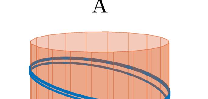
2003

of our full human potential, also referred to as flourishing [4, 5].

   While the components of these dimensions have been thoroughly studied (positive and negative
emotions and life satisfaction, for example), experts in the field of well-being point out the need for
theoretical models that offer a richer understanding of how the components of well-being interact,
account for the dynamical nature of well-being, and contribute to the multimethod approach of the
study of well-being [6].

   Motivated by this need, we take a very first step towards expressing the dynamical interrelation of
key components of well-being with a mathematical model.

   Since the components of happiness are certainly dynamic (our emotions for example), it is clear
that individual happiness also is dynamic and fluctuates over time. This is where mathematical
modelling becomes relevant. A continuous dynamical mathematical model can help us understand the
effects of the different determinants of happiness on its temporal dynamics, which in turn may provide
guidelines for making meaningful life changes to better our well-being. This mathematical approach
is illustrated in the pioneering dynamical model of happiness developed by Sprott [7], which
describes the dynamics of a person’s happiness in response to external events. While the model
successfully captures some hedonic aspects of happiness, it does not account for the multidimensional
nature of happiness and its derivation is, to a certain degree, arguable. First, the model’s derivation is
not based on any of the current views of well-being but simply on the assumption that the dynamics of
an individual’s happiness is equivalent to a like-dislike interaction among two individuals. Second,
the model supports a view where human beings are seen as passive individuals subjected to external
events, which according to positive psychology, is what led psychology in the past to become a
“victimology” [5, 8]. As a consequence, the model concludes that sustained happiness is unrealistic as
it would require an ever-increasing set of positive events for an individual to experience lasting
happiness.

    In this work, we overcome such limitations and develop a more comprehensive mathematical model
of happiness based on current positive psychology views of well-being where individuals are not seen
as victims of external forces but as proactive and self-determined beings who can master their well-
being and potentially achieve lasting happiness [5, 8]. The formulation of the model is based on a set
of theory-led assumptions which translate into a coherent definition of happiness and a description of
its dynamics with a nonlinear system of ordinary differential equations.

   The dynamics of the model offer insights into the role that emotions play in our happiness, the
reasons why we struggle to attain sustainable happiness and why we are often left treading the
hedonic treadmill and oscillating around a stable level of well-being in a hedonic homeostasis [3, 9].
Moreover, the model stability analysis indicates that lasting happiness may be achievable by
developing constant eudaimonic emotions or human altruistic qualities that overcome the boundaries
of the hardwired homeostatic hedonic system; in mathematical terms, this process of overcoming the
hedonic homeostasis is expressed as distinct dynamical bifurcations. This mathematical description is
consistent with the idea that eudaimonic well-being is beyond the boundaries of hedonic
homeostasis [10, 11].

Mathematical Biosciences and Engineering                                     Volume 19, Issue 2, 2002–2029.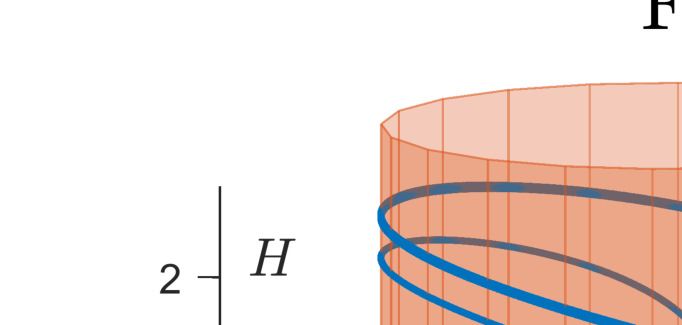
2004

2. Mathematical model

    One innovative and plausible aspect of Sprott’s dynamical model is that it defines happiness as a
rate of change [7]; initially, the rate of change of the emotion love. Although this approach has not
been derived from basic psychological principles and reducing happiness to love does not account for
its complexities, linking happiness to a rate of change is - as we shall see - a meaningful proposition
for the mathematical dynamical description of happiness.
    Indeed, the idea of happiness being a rate of change, and in particular, the rate of change of
satisfaction, is known to both Psychology and Philosophy. In the context of goal and discrepancy
theory, Carver and Scheier [12] suggested that the rate of change of satisfaction, also referred to as the
rate of change of progress towards a goal [5], rather than satisfaction itself, determines the experience
of happiness. Here, satisfaction is understood to be determined by the discrepancy or gap between
one’s present perceived reality and what one aspires or thinks one deserves [13–16]. As the
discrepancy decreases, the satisfaction increases.
    Interestingly, this idea of happiness being the rate of change of satisfaction also has philosophical
roots dating back to the nineteenth century. In particular, Schopenhauer [17] described human
happiness not as satisfaction per se but as the quick transition from wish and will striving to
satisfaction and from satisfaction to a new wish; in other words, happiness is described as the rate of
change of satisfaction.
    Perhaps the greatest challenge in developing a dynamical model for happiness is the need of clearly
defining happiness. Thus, for this purpose and using the idea of happiness as the rate of change of
satisfaction, we would like to describe mathematically the level of an individual’s happiness, H, as
                                                      dC(t)
                                             H(t) =         ,                                         (2.1)
                                                       dt
for a variable C (still to be determined) that could reflect the levels of an individual’s satisfaction or
contentment.
    The exact definition of the variable C and its range of values will become apparent as we develop
the mathematical model to describe an individual’s happiness over time. In order to build the model
we need to identify the main factors or ‘forces’ causing changes in the levels of happiness. From a
positive psychology perspective, emotions play a crucial role in an individual’s well-being. In
particular, positive emotions increase levels of well-being while negative ones decrease levels of
well-being [18–20]. Thus, both positive and negative emotions are driving ‘forces’ on the levels of an
individual’s happiness, and if F(t) denotes the intensity of emotions being experienced (affect), it is
reasonable to assume that
                                              dH(t)
                                                      = F(t) ,                                       (2.2)
                                                 dt
    Note that this basic model for the dynamics of happiness implies that if F(t) > 0 (the emotion being
experienced is positive), then dH(t)
                                 dt
                                     > 0 and the levels of happiness increase. Analogously, if F(t) < 0
(the emotion being experienced is negative), then dH(t)dt
                                                          < 0 and the levels of happiness decrease. This
is consistent with the positive psychology view that positive/negative emotions increase/decrease the
levels of well-being.
    In order to unfold the structure of F(t), it is necessary to consider not only our human emotional
inputs but also other well known mechanisms acting on these emotional inputs. In particular, using

Mathematical Biosciences and Engineering                                     Volume 19, Issue 2, 2002–2029.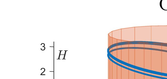
2005

information from adaptation, discrepancy, and goal-oriented theories, we will see in the next sections
that
                                       F(t) = Fe + Fd + Fr ,                                     (2.3)
where Fe , Fd , and Fr denote the emotional force, the hedonic damping, and the homeostatic restoring
force, respectively.

2.1. Emotional force
    Although there seems to be a clear consensus that positive emotions increase levels of well-being
and that negative ones decrease them, the fact that there are different classification systems and
measurement tools for positive and negative emotions [21–23] can pose a challenge not only for
defining what a positive or negative emotion is but also for determining the relative intensity of
positive and negative emotions. For this reason, and for the sake of developing a simple and
understandable model for happiness, we will define the emotional force Fe (t) as the overall intensity
of an individual’s emotions that arise at time t.
    If the overall intensity of emotions at a particular time is positive, i.e., Fe (t) > 0, we will refer to
it as a positive emotional force or input, and if the overall intensity of emotions at a particular time
is negative, i.e., Fe (t) < 0, we will refer to it as a negative emotional force or input. Thus, from Eq
(2.2), we notice that positive emotional inputs have the potential to increase a person’s happiness and
negative ones the potential to decrease it. However, we shall see that the impact of these emotional
inputs on the actual experience, F(t), of these emotions is affected by intrinsic human mechanisms of
adaptation and self-preservation.

2.2. Hedonic damping
    One of the mechanisms involved in reducing the impact of emotional inputs is known as hedonic
adaptation [24, 25]. This psychological process allows human beings to adapt to both favorable and
unfavorable circumstances and appears to reduce the affective impact of emotional inputs. For example,
when facing favorable circumstances that elicit positive emotions, which in turn can cause an increase
in the levels of happiness, the hedonic adaptation mechanism will reduce this effect and try to prevent
intense emotions causing euphoric states. Analogously, when unfavorable circumstances elicit negative
emotions, which can cause a decrease in the levels of happiness, the hedonic adaptation mechanism will
reduce this effect and try to prevent intense negative emotions causing depressive states. Therefore, it
is reasonable to describe the hedonic adaptation mechanism with the following hedonic damping term,
Fd , that reduces the impact of emotional inputs on a person’s levels of happiness:

                                                     dC
                                           Fd = −β      = −βH ,                                         (2.4)
                                                     dt
where β > 0 denotes the hedonic damping.

2.3. Well-being homeostatic system
   Another intrinsic psychological mechanism to be considered in the model is the subjective well-
being or hedonic homeostatic system that attempts to keep us with a positive view of ourselves by trying
to bring us to an equilibrium set-point of satisfaction [16, 26]. In order to describe this homeostatic

Mathematical Biosciences and Engineering                                       Volume 19, Issue 2, 2002–2029.
2006

system mathematically, we will consider some aspects of discrepancy and goal-oriented theories. In
particular, we will assume that the function of emotions is to help us progress towards a goal [22, 27];
the closer to the goal, the higher the satisfaction, i.e., the lesser the distance between our perceived
reality and where we would like to be [12]. In the context of discrepancy and goal-oriented theories,
we are continuously assessing our level of satisfaction. In the presence of discrepancy we adjust our
emotional response in the hope of getting closer to the goal and, in consequence, feeling satisfied [12].
    Under these assumptions, if the set-point level of satisfaction (which helps us keep a positive view of
the self) is perturbed, the hedonic homeostatic system will try to restore our stable level of satisfaction.
Thus, any emotional effort towards a goal will be affected by this restoring homeostatic system.
    Moreover, one basic notion that characterizes the hedonic homeostatic system is that goal
achievement is analogous or equivalent to a return to equilibrium [9]. Thus, two scenarios are
possible when an emotional input intends to move us towards a goal and the set-point of satisfaction is
perturbed, namely, the goal might not be achieved and the homeostatic system will bring us back to
the equilibrium set-point of satisfaction, or the goal is achieved and we also return to the equilibrium
set-point of satisfaction. Thus, the homeostatic system has a cyclic or periodic aspect to it with
respect to the levels of satisfaction. As we would like to capture this cyclic behaviour with a simple
periodic function, we describe the full mechanism of the hedonic homeostatic system with the
following homeostatic restoring force

                                           Fr = − sin(C) + p s ,                                       (2.5)

where C ∈ (−π, π], as we will see shortly, is a state variable that describes indirectly the level of
satisfaction, and the parameter p s , where −1 < p s < 1, will determine the stable or set-point level of
satisfaction.
    To appreciate the mathematical description of this homeostatic restoring force, illustrated in
Figure 1, we summarize its significant features and implications as follows:

     Figure 1. Homeostatic restoring force. A: The possible values for the discrepancy when
     C s < C(t) < π and −π < C(t) < C s are illustrated with solid and dashed blue and red
     lines, respectively. B: The blue and red trajectories describe, respectively, an adequate and
     an inadequate progress towards a goal.

Mathematical Biosciences and Engineering                                      Volume 19, Issue 2, 2002–2029.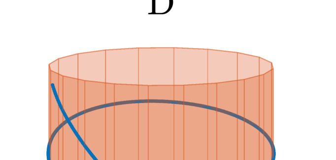
2007

  1) Given the periodic nature of the of the hedonic homeostatic system with respect to the levels
     of satisfaction, we restrict the domain of the homeostatic restoring force, Fr , to (−π, π], where
     C = −π is identified with C = π.
  2) There are two C-intercepts of Fr = − sin(C) + p s ; one closer to C = 0, denoted as C s , and one
     further away, denoted as Cu . In the following sections, we will see that C s represents a stable level
     of satisfaction, whereas Cu is an unstable steady state.
  3) Being away from the equilibrium C s at a particular time t places people in a position of
     dissatisfaction or discontentment, and they might aspire to a new state of satisfaction. For
     example, if C s < C(t) < Cu for a particular time t, the distance or discrepancy to a new state of
     satisfaction could be given by 2π + C s − C(t); however, a person might not aspire to that new
     state of satisfaction, in which case the discrepancy could be C(t) − C s (see Figure 1A). In
     general, if we represent each of these two different choices (aspiring or not aspiring to a new
     state of satisfaction) with m ∈ {0, 1}, the discrepancy D(t) at a particular time is determined by
     how far a person is to the equilibrium set-point of satisfaction C s in the following way:
     Case i. When C s ≤ C(t) ≤ π,

                                           D(t) = 2πm − (−1)m (C s − C(t)) .                             (2.6)
       This case is illustrated with the blue lines in Figure 1A.
       Case ii. When −π < C(t) < C s ,

                                           D(t) = 2πm + (−1)m (C s − C(t)) .                             (2.7)
       This case is illustrated with the red lines in Figure 1A.
       Note that D(t) ∈ [0, 2π]; the closer D(t) is to 0 the more satisfaction there is, and the closer D(t)
       is to 2π, the more dissatisfaction there is.
  4)   The magnitude of the restoring homeostatic force describes the adjustment needed in our
       emotional response to progress towards a new state of satisfaction or goal.
  5)   The progress towards a state of satisfaction reduces the discrepancy D(t) and can be either
       adequate or inadequate [12]. In the first case, dCdt
                                                              = H > 0, and in the second case, dC dt
                                                                                                     =H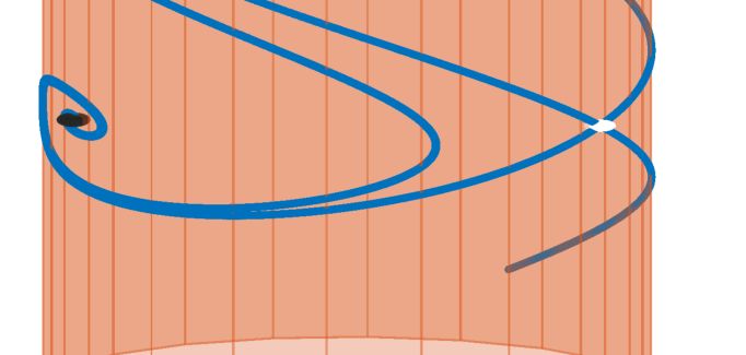
2008

    of satisfaction will be achieved), and to (C s , Cu ) as a range of low certainty. The behaviour within
    these ranges is consistent with the psychological view that contentment arises under conditions
    that include high certainty and low effort [28]. Note that this ideal dynamics, along the blue
    trajectory in Figure 1B, describes an adequate progress towards a goal, is obtained through a
    positive emotional force, and results in the experience of happiness ( dC   dt
                                                                                   = H > 0).
 8) Analogously, we could describe an inadequate progress towards a new state of satisfaction or
    goal. This dynamics is represented with the red trajectory in Figure 1B.
 9) If Fe (t) ≥ 1 − p s for a particular time t, we can think of the positive emotion at that time as being
    eudaimonic or flourishing in nature as it tries to overcome the homeostatic system in a positive
    way. This mathematical interpretation of an eudaimonic emotion is consistent with the positive
    psychology view that eudaimonic feelings overcome the limits of hedonic homeostasis [11].
    Similarly, if Fe (t) ≤ −1 − p s for a particular time t, we can think of the negative emotion as being
    destructive in nature as it tries to overcome the homeostatic system in a negative way.
10) The parameter p s can be interpreted as a genetic parameter determining the stable set-point level
    of satisfaction C s . Note that the higher the value of this set-point related parameter p s , the wider
    the range of high certainty; or equivalently, the narrower the range of low certainty. In other
    words, an individual with a high value of p s has a homeostatic goal-oriented mechanism that
    provides favorable conditions for an adequate progress towards a goal.

2.4. The full model
   Having unfolded the structure of the intensity of the affect F(t), we substitute its components given
by the emotional force, Fe , the hedonic damping, Fd , and the homeostatic restoring force, Fr , into
equation Eq (2.2), to obtain
                                   dH      dC(t)
                                      = −β       − sin(C) + p s + Fe (t) .                              (2.8)
                                   dt       dt
    Taking into account Eq (2.1), we can rewrite this last expression as the following second-order
differential equation describing the dynamics of happiness,
                                    d 2C    dC
                                       2
                                         +β    + sin(C) = p s + Fe (t) ,                                (2.9)
                                    dt      dt
where C ∈ (−π, π] is a state variable that describes indirectly the level of satisfaction, H = dC  dt
                                                                                                      denotes
the level of happiness, β > 0 is the hedonic damping coefficient, −1 < p s < 1 is the well-being set-
point related parameter, and Fe (t) is the emotional input. Interestingly, this equation, which describes
the dynamics of happiness, is the same differential equation used to describe the angular position of a
damped pendulum forced with a torque.
    Notice that since our interest is to describe the dynamics of happiness, H = dC  dt
                                                                                        , it is reasonable to
express the second-order differential equation given by Eq (2.9) as the following system of first-order
differential equations      " #0 "          #" # "                  # "       #
                             C        0 1 C                0             0
                                  =               +                  +          ,                      (2.10)
                             H        0 −β H         − sin(C) + p s     Fe (t)
where 0 denotes the derivative with respect to t, and (C, H) ∈ (−π, π] × (−∞, +∞). In other words, the
dynamics of happiness can be described on the surface of a cylinder (a cylindrical phase space) where

Mathematical Biosciences and Engineering                                       Volume 19, Issue 2, 2002–2029.
2009

the angular position describes indirectly the level of satisfaction and the height describes the level of
happiness.

   In the following sections, we will explore the effect of simple emotional inputs and different
parameter values for β and p s on the dynamics of happiness. In particular, we will show how
emotional impulses and increasing-decreasing positive emotional inputs can lead to a treadmill
dynamics of happiness, and investigate how the development of constant eudaimonic or flourishing
emotions can lead to lasting happiness. For the purpose of illustrating the results, all the solutions of
the happiness model in the following sections were obtained numerically using the ode solver ode45
in Matlab [29], which implements a Runge-Kutta method for the computations.

3. Model dynamics

3.1. Effect of an emotional impulse on the dynamics of happiness

  In order to understand the effect of an emotional impulse, we first analyze the basic dynamics of the
model in the absence of emotional inputs (i.e., Fe (t) = 0) by carrying out a linear stability analysis.

3.1.1. Dynamics in the absence of emotional inputs

   Assuming Fe (t) = 0 and, for the sake of simplicity, a well-being set-point related parameter p s = 0,
the proposed model for the dynamics of happiness given by Eq (2.10) becomes

                                     " #0 "    #" # "         #
                                      C    0 1 C          0
                                         =         +            ,                                       (3.1)
                                      H    0 −β H     − sin(C)

   By equating the vector field to zero we find that the fixed points (C ∗ , H ∗ ) of the system are given
by (C s , 0) = (0, 0) and (Cu , 0) = (π, 0). Notice that these fixed points are determined by the zeros of
the homeostatic restoring force. Moreover, by calculating the eigenvalues of the Jacobian matrix of the
vector field, it is easy to verify that (C s , 0) = (0, 0) is a spiral sink for 0 < β < 2 and stable node for
β ≥ 2, and that (Cu , 0) = (π, 0) is a saddle point. The phase portraits of these two cases are illustrated,
respectively, in Figure 2A,B.

Mathematical Biosciences and Engineering                                       Volume 19, Issue 2, 2002–2029.
2010
Figure 2. Dynamics in the absence of emotional inputs. A: Spiral sink (black) and saddle
point (white) of the happiness model with no emotional inputs given by Eq (3.1) when 0 <
β < 2. B: Stable node (black) and saddle point (white) of the happiness model with no
emotional inputs given by Eq (3.1) when β ≥ 2.
3.1.2. Dynamics in the presence of an emotional impulse
The importance of establishing first the dynamics of the happiness model with no emotional input,
given by Eq (3.1), stems from the fact that if we describe an emotional impulse as a dirac delta function
Fe (t − t0 ) = kδ(t − t0 ), where k and t0 are the intensity and the time of the emotional impulse, it can be
proved, using Laplace transforms, that solving the following system with an impulsive emotional input
for t > t0 ,
" #0 " #" # " # " # " # " #
C 0 1 C 0 0 C(t) 0
= + + ; = , t < t0 , (3.2)
H 0 −β H − sin(C) + p s kδ(t − t0 ) H(t) 0
is equivalent to solving the system with no emotional input
" #0 " #" # " # " # " #
C 0 1 C 0 C(t0 ) 0
= + ; = , (3.3)
H 0 −β H − sin(C) + p s H(t0 ) k
for t > t0 . Therefore, an emotional impulse causes a translation (equivalent to the intensity of the
impulse) in the happiness state variable of Eq (3.3) at the moment of the impulse. Figure 3A,B
illustrates how positive and negative emotional impulses perturb the stable steady state of the system
causing a sudden increase or decrease in the level of happiness, which then returns to its stable state.
Mathematical Biosciences and Engineering Volume 19, Issue 2, 2002–2029.2011
Figure 3. Dynamics in the presence of an emotional impulse. Solution (C(t), H(t)) on the
cylindrical phase space (top) and its happiness component H(t) (bottom) of the happiness
model given by Eq (3.2), where β = 1 and p s = 0, after applying an emotional impulse
Fe (t − 2) = kδ(t − 2) with A: k = 1.5, B: k = −1.5, and C: k = 4.5.
Also, Figure 3C shows that, if the intensity of the emotional impulse is high enough, it can
temporarily overcome the restoring homeostatic system, resulting in the solution going around the
cylindrical phase portrait before returning to the stable steady state.
Note that if our emotions comprise a series of positive and negative impulses, we will be
permanently subject to tread on the hedonic treadmill with ups and downs in our levels of happiness.
Moreover, emotional impulses describe particular emotional inputs that might not necessarily be the
most efficient way to progress towards a new state of satisfaction or to experience happiness.
3.2. Progressing towards a state of satisfaction through an increasing-decreasing positive emotional
input
In this section, we will describe how an increasing-decreasing positive emotion can overcome the
boundaries of the well-being homeostatic system temporarily, help us progress positively towards a
new state of satisfaction, and increase the time spent in a state of happiness. In particular, we consider
an emotional input of the form Fe (t) = k G(t), where
0, 0 ≤ t < ti ,
(t − ti )/(tm − ti ) , ti ≤ t ≤ tm ,
G(t) =
(3.4)
(t − t f )/(tm − t f ) , tm < t ≤ t f ,
0,
t>t ,
f
ti is the time when the positive emotion starts increasing, tm is the time when the maximum value k of
the emotion is reached and starts to decrease, and t f is the time when the positive emotion is no longer
present.
Mathematical Biosciences and Engineering Volume 19, Issue 2, 2002–2029.2012
This profile for Fe describes fairly reasonably how positive emotions can be regulated for the
purpose of reaching a new state of satisfaction. This is illustrated through an example in Figure 4.
Figure 4. Dynamics in the presence of an increasing-decreasing positive emotion. A: Graph
of the emotional input Fe (t) = kG(t), where G(t) is given by Eq (3.4), k = 1.5, ti = 2, tm = 12,
and t f = 17. Using this Fe (t), the solution of the happiness model given by Eq (2.10) with
β = 1, and p s = 0 is found and used to plot the temporal dynamics of B: the state variable
C(t), C: the happiness state variable H(t), D: the discrepancy D(t) given by Eq (2.6) and
Eq (2.7), and E: (C(t), H(t)) on the cylindrical phase space. F: Solution (C(t), H(t)) when the
parameters describing the positive emotional input Fe (t) are k = 1.5, ti = 2, tm = 10, and
t f = 15, i.e., the duration of the increasing positive emotional input is shorter.
In this example, after resting at a steady state a person has an initial desire to reach a new state of
satisfaction; we could say that this person is positively dissatisfied. At this moment (time ti = 2 in
Figure 4A), a positive emotion arises and increases in an effort to overcome the restoring homeostatic
force. Notice that the positive emotion reaches its maximum value at time tm = 12, and that C(tm ) > π/2
(Figure 4B); therefore, the positive emotion has already overcome the highest level of the homeostatic
restoring force (reached when C = π/2; see Figure 1). For this reason, the emotional response is
adjusted and starts to decrease until t f = 17. At this time, the effort of an emotional positive input is
not needed any longer as −π < C(t f ) < 0 (Figure 4B) and the positive homeostatic force will take the
person to the new state of satisfaction (Figure 1), represented, in this case, by the stable steady state
(C ∗ , H ∗ ) = (0, 0).
During this positive progression towards a new state of satisfaction, the levels of happiness are
positive (Figure 4C) and the discrepancy, described by Eq (2.6) and Eq (2.7), decreases (Figure 4D),
which in turn results in an increasing satisfaction. Given the transient, piecewise linear nature of the
emotional input in this case, the model was solved numerically first for the increasing part of the
emotional input, which then allowed us to have a new initial condition for solving the model with
the decreasing part of the emotional input, which in turn provided a new initial condition to solve the
Mathematical Biosciences and Engineering Volume 19, Issue 2, 2002–2029.2013
model with no emotional input.
The full dynamics of the happiness model on the cylindrical phase space is described in Figure 4E.
Note that the emotional input, interpreted as a response of the homeostatic restoring force, allowed the
solution to go around the cylindrical phase space. This is not the case if the positive emotion starts
to decrease before the maximum value of the homeostatic restoring is reached (let’s say, for example,
tm = 10 < 12); in other words, if the increasing positive emotional effort does not last long enough to
fully overcome the homeostatic restoring force. This results in an unsuccessful progress towards a new
state of satisfaction and the trajectory of the solution of the happiness model will not go completely
around the cylindrical phase space (Figure 4F).
We can see how the well-being homeostatic system plays a double role in the dynamics of happiness.
On the one hand, it tries to keep us content and with a positive view of ourselves by bringing us to an
equilibrium set-point of satisfaction. On the other hand, it challenges us to overcome its restoring force
in order to achieve a goal or new state of satisfaction. Therefore, the homeostatic system has a survival
function and also a human development function. By embracing the latter, we experience temporary
moments when the homeostatic system is broken; in other words, moments that allow us to flourish
and experience longer periods of happiness and eudaimonia.
If we assume that emotions are composed not only of discrete moments of positive and negative
impulses, but also of successful and unsuccessful attempts to adequately or inadequately progress
towards new goals or states of satisfaction, then our happiness level (driven mainly by these emotions)
will be subject to highs and lows (as shown in this and the previous section) and our well-being
experience could be described by a walk on the hedonic treadmill with moments of failures and
moments of flourishing.
Nonetheless, the dynamics of the model suggests that we can go beyond the hedonic treadmill, and
overcome the well-being homeostatic system. The following section is devoted to further explore this
dynamical behaviour by studying the effect that a constant positive emotional input can have on our
experience of happiness.
3.3. Dynamics of happiness in the presence of a constant positive emotional input
In the previous sections, we observed how the proposed model highlights the important role that
emotions play in the dynamics of the happiness and the satisfaction an individual experiences. In
particular, it demonstrates how emotional impulses and increasing-decreasing emotions that
temporarily overcome the well-being homeostatic system can leave us treading the hedonic treadmill
around positive and negative levels of happiness. Considering these dynamics, the question that
remains to be answered is whether lasting happiness is possible, or in other words, whether it is
possible to overcome the homeostatic system permanently. In order to answer this question, our focus
in this section will be on the effect that a constant positive emotional input can have in the dynamics
of happiness, i.e., we will consider an emotional input in Eq (2.10) of the form
Fe (t) = q , (3.5)
where q > 0.
Note that a constant positive emotional input directly and constantly affects the restoring
homeostatic force described by Eq (2.5). This becomes evident when we substitute the constant
Mathematical Biosciences and Engineering Volume 19, Issue 2, 2002–2029.2014
emotional input, given by Eq (3.5), into the happiness model described by Eq (2.10), which now
becomes " #0 " #" # " #
C 0 1 C 0
= + , (3.6)
H 0 −β H − sin(C) + p s + q
Notice that the restoring force, Fr , is affected by the constant emotional input q, and the C
component of the steady states of the happiness model given by Eq (3.6) is determined by the solution
of
Fr + Fe = − sin(C) + p = 0 , (3.7)
where p = p s + q .
Thus, we can interpret the development of a constant positive emotional input as a way of shifting
up the parameter p s and bringing up the homeostatic restoring force illustrated in Eq 2.5. In fact, it is
apparent that if a constant positive emotion is high enough such that p > 1 then the homeostatic system
can be permanently overcome. For the purpose of understanding how the overcoming of the hedonic
homeostatic system leads to lasting happiness, we start by carrying out a bifurcation analysis at p = 1.
Keeping in mind Eq (3.7), we note that there are two steady states, (C1 , 0) and (C2 , 0), of the
happiness model that come closer together as p increases and approaches 1. When p = 1, there is a
single equilibrium at (π/2, 0), which then disappears when p > 1. Moreover, as the Jacobian matrix of
the vector field of Eq (3.6), given by
" #
0 1
J= , (3.8)
− cos(C) −β
has a characteristic polynomial
p(λ) = λ2 + βλ + cos(C) , (3.9)
with roots p
λ1,2 = −β ± β2 − 4 cos(C) /2 , (3.10)
we conclude that when p approaches 1 from below the steady state (C1 , 0), where C1 > π/2, is a saddle
since λ1 < 0 < λ2 , and the steady state (C2 , 0), where C2 < π/2, is a stable node since λ1 , λ2 < 0.
This suggests that the homeostatic system can be broken through a saddle-node bifurcation as p
becomes greater than 1. Specifically, the steady state (π/2, 0) undergoes a saddle-node bifurcation at
the parameter value p = 1. In order to offer a rigorous proof of this bifurcation, we will show that
the (i) singularity, (ii) nondegeneracy and (iii) transversality conditions for a saddle-node bifurcation
to occur are met. These conditions are the basic assumptions of the saddle-note Theorem 8.6 and the
corresponding Corollary 8.7 stated by Meiss [30].
(i) Singularity:
To verify the singularity condition, we first introduce the following translation variables and new
parameter, respectively
z1 = C − π/2 , z2 = H , µ = p − 1 . (3.11)
Therefore, Eq (3.6) is transformed into the system
z01 = z2 = f1 (z1 , z2 ; µ) ,
(3.12)
z02 = −βz2 − cos(z1 ) + 1 + µ = f2 (z1 , z2 ; µ) ,
Mathematical Biosciences and Engineering Volume 19, Issue 2, 2002–2029.2015
with a Jacobian matrix for f (z1 , z2 ; µ) = ( f1 (z1 , z2 ; µ), f2 (z1 , z2 ; µ)) evaluated at (z1 , z2 ; µ) = (0, 0; 0)
given by " #
0 1
J f (0, 0; 0) = . (3.13)
0 −β
Thus, f (z1 , z2 ; µ) satisfies the singularity conditions
f (0, 0; 0) = (0, 0) , spec(J f (0, 0; 0)) = {0, −β; β , 0} . (3.14)
(ii) Nondegeneracy and (iii) Transversality:
Note that the system in Eq (3.12) can be rewritten in its matrix form as
" #0 " #" # " # " # " #
z1 0 1 z1 0 z1 0
= + = J f (0, 0; 0) + . (3.15)
z2 0 −β z2 − cos(z1 ) + 1 + µ z2 − cos(z1 ) + 1 + µ
To verify the nondegeneracy and transversality conditions, we need to transform Eq (3.15) into its
normal form. For this, we need to transform the Jacobian matrix of f at the origin, J f (0, 0; 0), into
Jordan normal form, JN , by finding the nonsingular matrix P of eigenvectors of J f (0, 0; 0), such that
JN = P−1 J f (0, 0; 0)P . (3.16)
Note that the eigenvectors corresponding to the eigenvalues 0 and −β of J f (0, 0; 0) are given by
(1, 0)T and (−1, β)T , respectively. Thus,
" # " #
1 −1 1 1/β
P= , P =
−1
, (3.17)
0 β 0 1/β
and "#
0 0
JN = P J f (0, 0; 0)P =
−1
. (3.18)
0 −β
Consider now the transformation of variables
" # " # " #" # " #
z1 x1 1 −1 x1 x1 − x2
=P = = , (3.19)
z2 x2 0 β x2 βx2
and its derivatives " #0 " #0
x z
P 1 = 1 . (3.20)
x2 z2
Substituting Eq (3.15) into Eq (3.20), multiplying both sides of the resulting equation from the left
by P−1 , and using Eq (3.19), we obtain the normal form of equation Eq (3.15)
" #0 " # " #
x1 x1 0
= P J f (0, 0; 0)P
−1
+P −1
, (3.21)
x2 x2 − cos(x1 − x2 ) + 1 + µ
which can be rewritten, using Eq (3.17) and Eq (3.18), as
" #0 "
g1 (x1 , x2 ; µ)
#" # " #
x1 0 0 x1
= + , (3.22)
x2 0 −β x2 g2 (x1 , x2 ; µ)
Mathematical Biosciences and Engineering Volume 19, Issue 2, 2002–2029.2016
where
g1 (x1 , x2 ; µ) = g2 (x1 , x2 ; µ) = − cos(x1 − x2 )/β + 1/β + µ/β , (3.23)
g(0, 0; 0) = (g1 (0, 0; 0), g2 (0, 0; 0)) = (0, 0) , (3.24)
and a Jacobian matrix of g(x1 , x2 ; µ) = (g1 (x1 , x2 ; µ), g2 (x1 , x2 ; µ)) evaluated at (x1 , x2 ; µ) = (0, 0; 0)
" #
0 0
Jg (0, 0; 0) = . (3.25)
0 0
Having the normal form in Eq (3.22) allows to show that the nondegeneracy condition
∂2 1
g1 (0, 0; 0) = , 0 , (3.26)
∂x1 2 β
and the transversality condition
∂ 1
g1 (0, 0; 0) = , 0 , (3.27)
∂µ β
in the saddle-node Theorem 8.6 and corresponding Corollary 8.7 in [30] are satisfied. Thus, we
conclude that the steady state (π/2, 0) of the happiness model given by Eq (3.6) undergoes a
saddle-node bifurcation at the parameter value p = 1. Also, if the constant emotional input is
sufficiently high such that p > 1, there are no equilibrium points and the hedonic homeostatic system
is permanently overcome. We will show that this leads to a stable state of lasting happiness described
by a limit cycle.
3.3.1. A state of lasting happiness
In order to prove the existence of a stable and lasting state of happiness when a sufficiently high
constant emotional input has been developed, we will prove the existence, uniqueness and global
stability of a periodic orbit with positive values of happiness around the cylindrical phase space when
p > 1.
Note that H 0 < 0 when H > (p + 1)/β and H 0 > 0 when H < (p − 1)/β. Then, if we choose constants
H1∗ < (p − 1)/β , and H2∗ > (p + 1)/β , (3.28)
all trajectories in the region H1∗ < H < H2∗ must, by Poincaré-Bendixson on the cylinder, stay in the
region and approach a periodic orbit as there are no fixed points when p > 1. This means that the
periodic orbit, indeed, exists. Moreover, this periodic orbit cannot be a libration (a periodic orbit that
does not circuit around the cylindrical phase space) as if it were, it should encircle a fixed point, but
again, there are no fixed points when p > 1. Therefore, the existing limit cycle is a rotation with values
of H > 0.
To prove that this limit cycle is unique, we first need to show that the following equality holds for
any rotation H(C), Z π
2πp
H(C)dC = . (3.29)
−π β
On the one hand, using Eq (3.6), we obtain that
Z π Z π Z π
dH
dC = (−βH − sin(C) + p) dC = −β HdC + 2πp . (3.30)
−π dt −π −π
Mathematical Biosciences and Engineering Volume 19, Issue 2, 2002–2029.2017
On the other hand, keeping in mind that the rotation is periodic with period denoted as T , we can also
compute the previous integral as
Z π Z T Z T Z T
dH dH dC dH dH
dC = dt = H dt = − H dt , (3.31)
−π dt 0 dt dt 0 dt 0 dt
which implies that
Z π
dH
dC = 0 . (3.32)
−π dt
Note that the substitution of Eq (3.32) into Eq (3.30), results in Eq (3.29).
Now, let us assume that there are two different rotations H1 (C) and H2 (C). As trajectories cannot
cross, we can also assume, without loss of generality, that H2 (C) > H1 (C) for all values of −π < C ≤ π.
Thus,
Z π Z π
H2 (C)dC > H1 (C)dC , (3.33)
−π −π
which contradicts Eq (3.29), and consequently, we conclude that the limit cycle for p > 1 is unique.
To prove that this limit cycle is globally asymptotically stable, note that H1∗ and H2∗ in Eq (3.28)
can have values arbitrarily negative and positive, respectively, Therefore, using again
Poincaré-Bendixson on the cylinder and the uniqueness of the limit cycle, we conclude that all the
trajectories of the happiness model approach the limit cycle asymptotically.
Thus, the globally attracting limit cycle with H > 0 that exists when p > 1 describes a state of
lasting happiness that can be achieved through the development of a constant positive emotion that
overcomes the hedonic homeostatic system.
Mathematical Biosciences and Engineering Volume 19, Issue 2, 2002–2029.2018
3.3.2. Path towards lasting happiness
Figure 5. Two-dimensional bifurcation diagram and homoclinic bifurcation. A: Graph of
Fr + Fe = − sin(C) + p for increasing values of p ; the black dots represent the C component
of the stable steady states and the white and grey dots the C component of the unstable ones.
B: βp-parameter space; the dashed blue line represents the expected saddle-node bifurcation
curve and the red lines denote the fixed values of β (0.5 and 1.5) where the p-values p1 = 0.5,
p2 = 0.6, p3 = 0.7, p4 = 0.99, p5 = 1, p6 = 1.1, p7 = 0.95, p8 = 1, and p9 = 1.1 were chosen
to illustrate all the possible bifurcations. C: Two-dimensional bifurcation diagram for the
happiness model given by Eq (3.6) on the βp-parameter space. D–F: Homoclinic bifurcation;
solution (C(t), H(t)) on the cylindrical phase space for the happiness model given by Eq (3.6)
with β = 0.5 and values of p = p s + q, chosen before the homoclinic bifurcation (p1 = 0.5
for D), at the homoclinic bifurcation (p2 = 0.6 for E), and after the homoclinic bifurcation
(p3 = 0.7 for F).
It is reasonable to think that the development of a constant positive emotion capable of overcoming
the hedonic homeostatic system, as illustrated in Figure 5A, can occur gradually until p > 1. In this
section, we shall see that this gradual development, which could be described by different values of
a constant positive emotion (and therefore, different values of p > 0), can go through two distinctive
paths leading to the state of lasting happiness explained in the previous section, namely, a path that
goes through a homoclinic bifurcation before encountering the saddle-node bifurcation at p = 1 and
another path that does not go through any bifurcation before encountering the saddle-node bifurcation
at p = 1.
Based on the bifurcation analysis carried out above, it is logical to consider a region in the βp-
parameter space, determined by p = 1, where the saddle-node bifurcation takes place, as shown in
Figure 5B. Within this region, the dynamics of the happiness model with a constant emotional input,
given by Eq (3.6), can be unfolded analogously to how the dynamics of the Josephson junction and
Mathematical Biosciences and Engineering Volume 19, Issue 2, 2002–2029.2019
the damped pendulum with a constant torque are unfolded [31–34]. This dynamics, which will be
illustrated shortly, is described by the two dimensional bifurcation diagram in Figure 5C, which shows
the curves where homoclinic, saddle-node and saddle-node on the invariant circle bifurcations occur in
the βp-parameter space. Given the relevance of the happiness model in offering a resulting dynamics
describing an achievable state of lasting happiness and the importance of the saddle-node bifurcation
experienced at p = 1 in identifying the threshold of the constant emotional input necessary to achieve
this state of lasting happiness, we focus the rigorous mathematical analysis on these significant aspects.
In particular, we carried out, in the previous sections, an in-depth saddle-node bifurcation analysis at
p = 1 and also a meticulous global stability analysis for the attracting limit cycle that exists for p > 1.
The rigorous study of the homoclinic bifurcation would be lengthy and would deviate from the main
narrative and scope of this manuscript. For this reason, we refer the reader interested in the thorough
details of such bifurcation to Levi and Hoppensteadt [31] and Guckenheimer and Holmes [32].
The homoclinic bifurcation curve in Figure 5C was generated numerically by carrying out
simulations of the happiness model in Eq (3.6) for starting values of β and p close to zero and close to
the line p = 4β/π to spot the homoclinic orbits. The reason for using this line is that Guckenheimer
and Holmes [32] derived a analytical approximation for the homoclinic bifurcation curve for values of
β close to zero and showed that this approximation is tangent to the line p = 4β/π as β approaches
zero. Thus, after graphing the homoclinic bifurcation curve in Figure 5C for the initial values of β and
p, we continued generating it by tracking the homoclinic orbit of the happiness model within
increments of length 0.05 for β until the homoclinic bifurcation curve touched p = 1.
In order to illustrate the dynamics of the happiness model with a constant emotional input, shown
in the βp-bifurcation diagram, we consider two fixed values for β (β = 0.5 and β = 1.5) and let p
vary across the homoclinic, the saddle-node and the saddle-node on the invariant circle bifurcation
curves. The particular values of p, shown in Figure 5B, were carefully chosen after having generated
Figure 5C, so that (i) p1 , p2 , and p3 lie, respectively, below, over, and above, the homoclinic bifurcation
curve, (ii) p4 , p5 , and p6 lie, respectively, below, over, and above, the saddle-node bifurcation curve
given by p = 1 with a pairing value of β such that p4 falls in a bistability region, and (iii) p7 , p8 , and
p9 lie, respectively, below, over, and above, the saddle-node on the invariant circle bifurcation curve
given by p = 1, with a pairing value of β such that p7 does not fall in a bistabilty region.
Homoclinic path towards lasting happiness.
Using β = 0.5 and letting p vary across the homoclinic bifurcation curve with values of p1 = 0.5,
p2 = 0.6, and p3 = 0.7, we can see in Figure 5D–F, how the dynamics of the happiness model varies
accordingly to these parameter values.
Figure 5D, obtained when p = p1 , describes the dynamics of the model before the homoclinic
bifurcation occurs, and therefore shows the existence of a stable fixed point and an unstable one (a
saddle). In this case, all the trajectories, except the ones starting at the saddle point or its stable
manifold, will go to the stable fixed point. This same dynamics is shared when the choice of parameter
values falls in the ‘stable fixed point’ region in Figure 5C.
Figure 5E, obtained when p = p2 , describes the dynamics of the model when the homoclinic
bifurcation occurs, and therefore shows the existence of a homoclinic curve that arises when one of the
branches of the unstable manifold of the saddle point joins one of the branches its stable manifold. This
dynamical behaviour is shared when the choice of parameter values lies on the homoclinic bifurcation
Mathematical Biosciences and Engineering Volume 19, Issue 2, 2002–2029.2020
curve in Figure 5C.
As p increases, for example when p = p3 , a stable limit cycle arises from the homoclinic bifurcation,
as shown in Figure 5F, creating a bistable dynamics, where some of the trajectories will be attracted to
the limit cycle and others to the stable fixed point. This dynamics occurs when the choice of parameter
values falls on the ‘bistability’ region in Figure 5C.
Notice, on the one hand, that if the constant positive emotional input Fe (t) = q is not high enough
to make p = p s + q greater than the p-values given by the homoclinic bifurcation curve, then the
dynamics of happiness will be determined by the stable steady state and will be subject to the well-
being homeostatic system just as in the previous sections. In other words, if this constant positive
emotional input is accompanied by a series of positive and negative impulses that perturb the stable
steady state, and by successful and unsuccessful attempts to achieve new states of satisfaction, a person
will be left treading the hedonic treadmill with ups and downs in the levels of happiness. However, it
is important to mention that even though the qualitative dynamics in this case does not differ to the one
described in the previous sections, the development of a constant positive emotion will always bring
the worthy benefit of lifting up the homeostatic restoring force, which puts an individual in a better
position to adequately progress towards new goals or states of satisfaction.
On the other hand, if the constant positive emotional input Fe (t) = q is high enough and p =
p s + q < 1 becomes greater than the p-values given by the homoclinic bifurcation curve, the bistability
dynamics will allow for the possibility of experiencing a ‘taste’ of lasting happiness even though the
well-being homeostatic system is not fully broken. This is represented by trajectories starting at a
certain region of the cylindrical phase space that are attracted to the stable limit cycle, which in turn
oscillates with positive values of happiness H (Figure 5F). We call this experience ‘shakable lasting
happiness’ as a negative emotional input can bring a person to points on the cylindrical phase space
leading to trajectories that are attracted to the stable steady state.
We refer to this possible progression in the development of a constant positive emotional input
passing through the homoclinic bifurcation curve as the homoclinic path towards lasting happiness.
Saddle-node path towards lasting happiness.
In order to follow the dynamics after the homoclinic bifurcation, we keep β = 0.5 and let p increase
across p = 1 with values p4 = 0.99, p5 = 1, and p6 = 1.1. Figure 6A–C show how the dynamics
of the happiness model varies according to these parameter values. Note that the choice p = p4 falls
in the ‘bistability’ region, and the model dynamics, described by Figure 6A, shares the same bistable
dynamical feature as the previous case (i.e., p = p3 ) but with the steady states closer together and the
stable fixed point becoming a stable node.
When p reaches the SN (saddle-node) bifurcation value p5 = 1, the stable node and the saddle
collide into a unique unstable fixed point (Figure 6B), which then disappears as p reaches values
greater than one, for example, p = p6 (Figure 6B), while the stable limit cycle, which came originally
from the homoclinic bifurcation, persists.
A similar, but mathematically slightly different, behaviour occurs when the value of the hedonic
damping coefficient β is too high (for example, β = 1.5) for the model dynamics to undergo a
homoclinic bifurcation. In this case, the only path to lasting happiness is through p crossing the SNIC
(saddle-node on the invariant circle) bifurcation value. This is described in Figure 6D–F as p crosses
the saddle-node bifurcation curve with values of p7 = 0.95, p8 = 1, and p9 = 1.1. In this case, a limit
Mathematical Biosciences and Engineering Volume 19, Issue 2, 2002–2029.2021
cycle did not exist before the saddle-node bifurcation occurred, but since this bifurcation takes place
on the invariant circle formed by the two branches of the unstable manifold of the saddle with the
stable steady state (Figure 6D, E), a stable limit cycle arises as p becomes greater than one
(Figure 6F).
Thus, for both these saddle-node bifurcation cases (SN and SNIC), if a person develops a constant
emotional input q > 0, such that p = p s + q > 1, there will be a stable limit cycle oscillating with
positive values of happiness H attracting all the trajectories of the model, as proved in Section 3.3.1.
In other words, the person fully overcomes the well-being homeostatic system and guarantees the
experience of lasting happiness.
Figure 6. SN (Saddle-Node) and SNIC (Saddle-Node on the Invariant Circle) bifurcations.
A–C: SN bifurcation; solution (C(t), H(t)) on the cylindrical phase space for the happiness
model given by Eq (3.6) with β = 0.5 and values of p = p s + q, chosen before the SN
bifurcation (p4 = 0.99 for A), at the SN bifurcation (p5 = 1 for B), and after the SN
bifurcation (p6 = 1.1 for C). D–F: SNIC bifurcation; solution (C(t), H(t)) on the cylindrical
phase space for the happiness model given by Eq (3.6) with β = 1.5 and values of p = p s + q,
chosen before the SNIC bifurcation (p7 = 0.95 for D), at the SNIC bifurcation (p8 = 1 for
E), and after the SNIC bifurcation (p9 = 1.1 for F).
Low and high hedonic damping progression towards lasting happiness.
In order to further describe the path towards lasting happiness through the development of a constant
positive emotional input, we graph the one-dimensional bifurcation diagrams with respect to p when a
person is characterized with low and high hedonic damping coefficients.
Figure 7A,B shows the bifurcation diagrams with respect to the parameter p for the state variables
H and C, respectively, when a person is characterized with a low β = 0.5, which can be interpreted as
a value characterizing a person with high sensitivity to emotional inputs. The presence of a bistability
region as p passes the value p = 0.6 becomes evident in Figure 7A, which shows how a stable limit
Mathematical Biosciences and Engineering Volume 19, Issue 2, 2002–2029.2022
cycle (with maximum and minimum values described by the red and blue curves in the figure) appears
after the homoclinic bifurcation. This limit cycle persists beyond the occurrence of the SN bifurcation
at p = 1 (shown in Figure 7B for the phase variable C), which guarantees the experience of lasting
happiness.
5 2
limit cycle minimum Stable fixed point limit cycle minimum
limit cycle maximum Unstable fixed point limit cycle maximum
4 fixed point fixed point
1.5
3
/2 1
2
0.5
1
0 0 0
0 0.6 1 1.5 2 0 0.5 1 1.5 0 0.5 1 1.5 2
1 2.5 3
2 2.5
0.5 1.5 2
1 1.5
0 0.5 1
0 0.5
-0.5 -0.5 0
0 5 10 15 20 25 0 5 10 15 20 25 0 5 10 15 20 25
Figure 7. One-dimensional bifurcation diagrams and bistable dynamics. One-dimensional
bifurcation diagrams of the happiness model given by Eq (3.6) with respect to the parameter
p = p s + q for A: the state variable H when β = 0.5 , B: the state variable C when β = 0.5 ,
and C: the state variable H when β = 1.5 . Solution H(t) of the happiness model given by
Eq (3.6) with β = 0.5, and D: a parameter p = 0.5 , and initial condition (C(0), H(0)) =
(arcsin(p), 0) , E: a parameter p = 0.7 and initial conditions (C(0), H(0)) = (arcsin(p), 1)
and (C(0), H(0)) = (arcsin(p), 1.5) (blue and red curves, respectively), and F: a parameter
p = 1.1 , and initial condition (C(0), H(0)) = (0, 0) .
An interesting phenomenon indicated by the arrows in the bifurcation diagram of Figure 7A is that
of hysteresis. If the value of p and H are initially small, then as p increases, H will continue to be
attracted to the fixed point (H = 0) even after passing the homoclinic bifurcation value p = 0.6. When
p exceeds the saddle-node bifurcation value p = 1, the happiness H will jump up into a positive state
given by the limit cycle. If at this state p is brought back down below p = 1, the happiness H will
not jump back down or be attracted to the fixed point, instead it will be attracted to the stable limit
cycle that persisted for values less than 1. The H values of the limit cycle will tend to zero as p
decreases towards the homoclinic bifurcation value p = 0.6. Thus, if a person develops a positive
constant emotional input that makes p > 1 and overcomes the well-being homeostatic system, then
the hysteretic phenomenon allows the person to relax the value of p below the saddle-node bifurcation
value, regain the well-being homeostatic system and still enjoy being in a state of lasting happiness
described by the positive limit cycle.
In Figure 7C, we plot the bifurcation diagram for the happiness variable H when the hedonic
damping β = 1.5, which can be interpreted as a value characterizing a person less sensitive to
Mathematical Biosciences and Engineering Volume 19, Issue 2, 2002–2029.2023
emotional inputs (i.e., a person who is not as impacted by emotional inputs). Note that the progress
towards lasting happiness does not go through a homoclinic bifurcation, and a hysteretic phenomenon
is not present. The bifurcation diagram for C, in this case, would look like the one in Figure 7B, and
as mentioned before, the path to lasting occurs as p passes the SNIC bifurcation at p = 1.
We could, therefore, think that having a low hedonic damping β is advantageous as it would allow
for the possibility of experiencing a shakable sustainable happiness due to the bistable dynamics
arising from the homoclinic bifurcation. This is true; however, a low hedonic damping also poses the
disadvantage of ups and downs between positive and negative values of happiness as a response to
emotional disturbances around a spiral fixed point. The reverse situation applies when the hedonic
damping β is high; the advantage of reducing the impact of emotional inputs is having a more steady
return to the fixed point, and the disadvantage would be the absence of bistable dynamics.
Nonetheless, regardless of how well an individual reduces the impact of emotional inputs, the
development of a constant eudaimonic or altruistic emotion will overcome the well-being homeostatic
system and will lead to a path of lasting happiness. Once this altruistic state is reached, the concept of
a personal satisfaction described by the happiness model is dissolved as the well-being homeostatic
system is overcome and the fixed points determined by it are now nonexistent.
The progression of regulating our emotional input in an increasing positive and constant fashion
is represented by different temporal dynamics of happiness in Figure 7D–F for increasing values of
p = p s + q chosen to be below the homoclinic bifurcation value (Figure 7D), within the region of
bistability (Figure 7E), and above the saddle-node bifurcation value (Figure 7E).
Assuming a path towards lasting happiness through both the homoclinic and the saddle-node
bifurcations, the initial stage of this progression requires the development of a “not so high” constant
positive emotional input that falls in the “stable fixed point” region of the two-dimensional bifurcation
diagram represented in Figure 5C. At this stage, the main gain is the beneficial effect of lifting up the
restoring homeostatic system, which in turn places a person in a better position to achieve new states
of satisfaction or goals. An example of the temporal dynamics of happiness at this stage is given in
Figure 7D. The next stage would require the development of a “high enough” constant positive
emotional input that falls into the “bistability” region of the bifurcation diagram and allows for the
possibility to experience a “taste” of lasting happiness. An example of the two possible temporal
dynamical behaviours for happiness is given in Figure 7E. Finally, the last stage in the path towards
lasting happiness requires the development of a “high” and “altruistic” constant positive emotional
input that falls into the “stable limit cycle” region of the bifurcation diagram, overcomes the
well-being homeostatic system, and guarantees the experience of lasting happiness, as illustrated in
Figure 7F and proved in Section 3.3.1.
4. Discussion
As the purpose of the proposed model is to increase our understanding of the dynamical nature of
happiness and gain insight into the theoretical underpinnings of well-being components, its validity
will rest not only on its ability to fit empirical data but also on its ability to predict qualitatively
expected conceptual outcomes related to well-being. We can think of this as a distinction between the
quantitative and the qualitative predictive ability of the model. The focus of this section is to offer an
initial discussion of these two aspects.
Mathematical Biosciences and Engineering Volume 19, Issue 2, 2002–2029.You can also read