A Stacking Ensemble Deep Learning Model for Bitcoin Price Prediction Using Twitter Comments on Bitcoin
←
→
Page content transcription
If your browser does not render page correctly, please read the page content below
mathematics

Article
A Stacking Ensemble Deep Learning Model for Bitcoin Price
Prediction Using Twitter Comments on Bitcoin
Zi Ye † , Yinxu Wu †                  , Hui Chen     , Yi Pan, Qingshan Jiang *

                                          Shenzhen Institute of Advanced Technology, Chinese Academy of Sciences, Shenzhen 518055, China;
                                          zi.ye@siat.ac.cn (Z.Y.); wyx83coria@hotmail.com (Y.W.); hui.chen1@siat.ac.cn (H.C.); yi.pan@siat.ac.cn (Y.P.)
                                          * Correspondence: qs.jiang@siat.ac.cn
                                          † These authors contributed equally to this work.

                                          Abstract: Cryptocurrencies can be considered as mathematical money. As the most famous cryp-
                                          tocurrency, the Bitcoin price forecasting model is one of the popular mathematical models in financial
                                          technology because of its large price fluctuations and complexity. This paper proposes a novel
                                          ensemble deep learning model to predict Bitcoin’s next 30 min prices by using price data, technical
                                          indicators and sentiment indexes, which integrates two kinds of neural networks, long short-term
                                          memory (LSTM) and gate recurrent unit (GRU), with stacking ensemble technique to improve the
                                          accuracy of decision. Because of the real-time updates of comments on social media, this paper uses
                                          social media texts instead of news websites as the source data of public opinion. It is processed by lin-
                                          guistic statistical method to form the sentiment indexes. Meanwhile, as a financial market forecasting
                                          model, the model selects the technical indicators as input as well. Real data from September 2017 to
                                          January 2021 is used to train and evaluate the model. The experimental results show that the near-real
                                time prediction has a better performance, with a mean absolute error (MAE) 88.74% better than the

                                          daily prediction. The purpose of this work is to explain our solution and show that the ensemble
Citation: Ye, Z.; Wu, Y.; Chen, H.;
                                          method has better performance and can better help investors in making the right investment decision
Pan, Y.; Jiang, Q. A Stacking
                                          than other traditional models.
Ensemble Deep Learning Model for
Bitcoin Price Prediction Using Twitter
                                          Keywords: cryptocurrencies; forecasting model; financial technology; ensemble learning; Bitcoin
Comments on Bitcoin. Mathematics
2022, 10, 1307. https://doi.org/
                                          price prediction
10.3390/math10081307
                                          MSC: 68Uxx; 68U35
Academic Editors: Maria Del Mar
Miralles-Quirós and José Luis
Miralles-Quirós

Received: 27 February 2022                1. Introduction
Accepted: 10 April 2022                        Bitcoin is the first and the most important cryptocurrency. It is a ledger application
Published: 14 April 2022                  based on blockchain, cryptography and peer-to-peer technology. In the field of financial
Publisher’s Note: MDPI stays neutral
                                          technology, many mathematical models are developed to forecast Bitcoin’s future price.
with regard to jurisdictional claims in   These models can provide investment advice for quantitative investors.
published maps and institutional affil-        Similar to other assets, such as stocks [1,2] and commodities, Bitcoin price forecasts are
iations.                                  a series of continuous predictions because Bitcoin prices also change over time. One major
                                          difference between Bitcoin and a stock is that stocks trade only at certain times on weekdays,
                                          but the Bitcoin market typically operates around the clock, and investors can buy or sell
                                          Bitcoin all day, which may result in Bitcoin price fluctuations at unpredictable times. We can
Copyright: © 2022 by the authors.         learn the stock price prediction method and use it to predict the price of Bitcoin. To address
Licensee MDPI, Basel, Switzerland.        the time series problem of Bitcoin prices, two types of models have mainly been used in
This article is an open access article    previous works: traditional time series models, such as autoregressive comprehensive
distributed under the terms and           moving average (ARIMA) [3] and generalized autoregressive conditional heterovariance
conditions of the Creative Commons
                                          (GARCH) [4]. Another is machine learning models, such as random forest (RF), and deep
Attribution (CC BY) license (https://
                                          learning networks, such as recurrent neural networks (RNN), long short-term memory
creativecommons.org/licenses/by/
                                          (LSTM), and gated recurrent units (GRU) [5].
4.0/).

Mathematics 2022, 10, 1307. https://doi.org/10.3390/math10081307                                           https://www.mdpi.com/journal/mathematics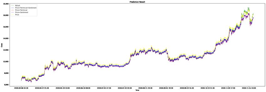
Mathematics 2022, 10, 1307                                                                                             2 of 21

                                   According to a study by the American Institute of Economic Research (AIER), globally
                             influential news and sentiment can drive large fluctuations in the price of Bitcoin [6]. Some
                             research uses sentiment analysis based on Twitter data to predict the price of Bitcoin [5,7]. It
                             is effective to explore people’s reactions to Bitcoin from tweets since Twitter is an incredibly
                             rich source of information about how people are feeling about a given topic. Previous
                             research methods of sentiment analysis based on Bitcoin-related comments can be divided
                             into two types: dictionary-based methods, such as valence aware dictionary and sentiment
                             reasoner (VADER) [8], and machine learning-based methods, such as RF [7], hard voting
                             classifiers [5], deep learning-based classifiers [9], and other specific analyzers [10].
                                   However, the current research still has some limitations: Firstly, in most previous
                             works, only historical data are used as the input data of the prediction model, which ignores
                             that prices are also affected by unexpected factors in price data. Secondly, sentiment analysis
                             simply categorizes every tweet or comment as positive, neutral or negative and then creates
                             a simple statistic, which loses much emotional detail and is not conducive to learning how
                             different levels of sentiment affect prices. Thirdly, a single model such as ARIMA, LSTM,
                             or GRU, is employed by most previous methods. To solve the existing limitations, this
                             paper proposed following aspects: Firstly, considering the financial nature of Bitcoin, we
                             added the most commonly used technical indicators in traditional finance as predicting
                             input. Secondly, instead of using a simple statistical method to categorize the mood trend
                             of tweets, we used a linguistic method to process tweets about Bitcoin, which proved it
                             brought a higher accuracy. Thirdly, to improve the prediction results, a stacking ensemble
                             Deep Learning, combining LSTM and GRU, was trained to forecast the price of the next
                             time interval. The major steps are as follows. We proposed to use linguistic sentiment
                             analysis to categorize tweets and a stacking ensemble deep learning model to forecast the
                             price of the next time interval based on sentiment trend of tweets and technical indicators.
                             It combines multiple models to add a bias to the final prediction result, which will be offset
                             by the variance of the neural network, making the prediction of the model less sensitive to
                             the details of training data.
                                   The rest of this paper is organized as follows: Section 2 shows the previous related
                             work; Section 3 shows the whole methodology of this paper, including the data acquisition
                             step, data preprocessing step and stacking ensemble prediction model; Section 4 lists all the
                             experimental results and compares our method with common methods; Section 5 draws
                             the conclusion of this paper.

                             2. Related Work
                                  Many previous studies can mainly be divided into three main models and three main
                             data categories. The three models include: (1) statistical methods; (2) machine learning;
                             (3) ensemble learning. The three main data types are as follows: (1) price data, including
                             opening, highest, lowest, closing, trading volume, number of trades, quote asst volume
                             and other data; (2) technical indicators based on price data and indicators derived from
                             market technical statistics, such as moving average convergence divergence (MACD) and
                             relative strength index on balance volume (RSI OBV) statistics; (3) sentiment indicators
                             refer to the indicators calculated after natural language processing of text data from social
                             media during a certain time period; (4) other related data, such as blcokchain hashrate,
                             number of online nodes, active address, Google trends and other financial indexes.
                                  Early research into the price prediction of bitcoin were mostly based on the statistical
                             method. P. Katsiampa et al. [11] used price data, and certain types of GARCH models
                             have been used to calculate the daily closing prices between 18 July 2010 and 1 October
                             2016. As a result of the paper, AR-CGARCH is the best model. S. Roy et al. [4] used
                             price data and performed ARIMA, autoregressive (AR), and moving average (MA) models
                             on the time series dataset. The results of this paper used the ARIMA model to predict
                             the price of Bitcoin with an accuracy rate of 90.31%. Therefore, it can be said that the
                             best results are obtained using ARIMA. Ayaz et al. [12] used price data and only used
                             the ARIMA algorithm to predict the price of Bitcoin. To find the lowest mean square
Mathematics 2022, 10, 1307 3 of 21
error (MSE), the researchers used different fitting functions in the ARIMA algorithm and
found that the lowest MSE = 170,962.195. Because it avoids the use of scaling functions, this
result is different from those of other studies. In a recent paper [13], it proposed a general
method of user behavior analysis and knowledge pattern extraction based on social network
analysis. This method extracts relevant information from the blockchain transaction data in
a specified period, carries out statistics and builds an ego network, and extracts important
information such as active transaction addresses and different user groups. Using Ethereum
blockchain data from 2017–2018, the method was proved to be able to identify bubble
speculators. In 2021, R. K. Jana et al. [14] proposed a regression framework based on
differential evolution to predict bitcoin. They first decomposed the original sequence into
granular linear and nonlinear components using maximum overlapping discrete wavelet
transform, and then fitted polynomial regression with interaction (PRI) and support vector
regression (SVR) on both linear and nonlinear components to obtain the component-
wise projections.Apart from the previously introduced statistical methods, Jong-Min Kim
et al. [15] proposed to use linear and nonlinear error correction models to predict bitcoin log
returns, and compared with neural network, ARIMA and other methods. The experiment
was verified with the price data from 1 January 2019 to 27 August 2021. The results showed
that the error correction model was the best in all evaluation indexes, and MAE was as
low as 1.84, while other comparison models were all above 3.2. They also ran a Granger
causality test on 14 cryptocurrencies.
Over the past few decades, major advances in machine learning have allowed more
accurate methods to spread across the field of quantitative finance. A Bayesian neural net-
work model that uses blockchain information to predict the price of Bitcoin was proposed
by Jang et al. in 2017 [16]. Specifically, they use price data, blockchain data, economic
indices, currency exchange rates and more. Four methods were trained for price prediction
using price data, including logistic regression, support vector machine, RNN and ARIMA
models in [17]. As far as the prediction accuracy of these four methods is concerned,
ARIMA only has a 53% return on the next day’s price prediction, and the long-term perfor-
mance is poor, such as using the price prediction of the last few days to predict the price
of the next 5–7 days. The RNN consistently obtains an approximate accuracy of 50% for
up to 6 days. It does not violate the assumptions of the logistic regression-based model; it
can accurately classify only when there is a separable hyperplane with 47% accuracy. The
support vector machine has an accuracy rate of 48%. Shen et al. [18] used price data for
training the GARCH, simple moving average (SMA) and RNN (GRU) models. The GRU
model performs better than the SMA model with the lowest root MSE (RMSE) and mean
absolute error (MAE) ratios. Some researchers used price data, technical indicators and
a complex neural network called CNN-LSTM [19]. Compared with a single CNN and a
single LSTM model, the results are slightly improved, with the MAE reaching 209.89 and
the RMSE reaching 258.31. The stochastic neural network model has also been used to
predict the price of cryptocurrency [20]. The model introduces layer-wise randomness into
the observed neural network feature activation to simulate market fluctuations. It used
market transaction data, blockchain data, and Twitter and Google Trends data. A latest
research on cryptocurrencies by Wołk [21] used Google Trends and Twitter to predict the
price of cryptocurrencies by distinctive multimodal scheme. However, they used textual
data mechanically, unlike our article, which considers linguistic approaches to textual data.
In 2021, Jagannath et al. [22] proposed a Bitcoin price prediction method using data features
of users, miners, and exchanges. They also propose jSO adaptive deep neural network
optimization algorithm to speed up the training process. The model uses Bitcoin data from
2016 to 2020 for training and testing. The MAE value of LSTM is 2.90, while the MAE value
of this method is 1.89, thus effectively reducing the MAE value. A novel price prediction
model WT-CATCN was proposed in 2021 by Haizhou Guo et al. [23]. It utilizes Wavelet
Transform (WT) and Casual Multi-Head Attention (CA) Temporal Convolutional Network
(TCN) to predict cryptocurrency prices. The data input of the model is divided into three
categories: blockchain transaction information, exchange information, and Google Trends.Mathematics 2022, 10, 1307 4 of 21
Considering how widespread cryptocurrency information has become, Loginova proposed
a bitcoin price direction prediction method in 2021 that combined the sentiment analysis
model JST and TS-LDA [24]. They used market trading data as well as text data from
Reddit, CryptoCompare and Bitcointalk. The model was verified by using the data from 20
February 2017 to 6 April 2019. The accuracy of the model using JST and TS-LDA was 57%,
which was improved compared with the same model that was not used. For Dogecoin,
which has a huge market cap, Sashank Sridhar et al. proposed a multi-head attention-based
encoder–decoder model for a transformer model to predict its price [25]. It is verified using
real DOGE hourly transaction data from 5 July 2019 to 28 April 2021, with an R-squared
value of 0.8616 for the model. A more complex hybrid framework, DL-GuesS, was pro-
posed by Raj Parekh et al. for cryptocurrency price prediction [26]. This framework takes
into account its interdependence with other cryptocurrencies and market sentiment. The
model uses transaction data from different cryptocurrencies as input, along with Twitter
text. The model was validated using Bitcoin Cash data from March 2021 to April 2021, and
the model MSE value was as low as 0.0011.
Ensemble learning is also a popular method for forecasting. Using this approach,
researchers have been able to improve the accuracy and stability of predictions. Ahmed
Ibrahim [27] used price and sentiment data to predict Bitcoin prices by constructing an
XGBoost-Composite integrated model. A paper using price data to compare different
ensemble models, including averaging, bagging, and stacking was written in 2020 [28].
Among them, stacking has the best performance, but the blending ensemble was not used
in the paper. Other researchers used price data and integrated LSTM models after training
for different lengths of time (days, hours, and minutes) to obtain an integrated model that
was superior to each individual model [29].
Mainly inspired by Li and Pan [1], whose workflow is shown in Figure 1, this paper
designs a series of methods to avoid these current limitations: (1) more data sources are
used as input; (2) linguistic methods are used for sentiment analysis to replace the simple
statistical methods used in most papers; (3) one kind of ensemble model is used for training
and prediction.
Figure 1. The workflow for forecasting stock using news data in Li [1].
However, due to different data sources, the methods proposed in this paper are
somewhat different from those proposed in Li [1]. The differences of specific data sources
are as follows:
1. There is less news about digital currency than stocks, which means there are not
many reports about digital currency in the news, which is not enough to support our
real-time prediction, so we chose social media.
2. Digital currencies are traded 24 h a day and comments on Twitter are live 24 h a day,
so real-time comments on Twitter can be very effective for price forecasting.Mathematics 2022, 10, 1307 5 of 21
3. Li’s work uses two data sources, price and news, to predict price. Considering
the financial properties of digital currency, we use price, comments on Twitter and
technical indicators to predict price.
4. Data preprocessing methods are also different: The text data used in Li [1], namely
news data, does not need to be cleaned and can be scored directly by VADER. More-
over, the Twitter data we obtain from crawlers is very dirty, such as pictures, links,
etc., which need to be cleaned.
3. Methodology
In this paper, sentiment indicators are combined with Bitcoin price data to predict the
future price. The proposed model workflow is shown in Figure 2. In step 1, Twitter data
are collected and processed to form a structured Twitter date, which is in CSV format. In
step 2, the structured Twitter date is sent to the sentiment calculation program. The SGSBI
and SGSDI are calculated and attached to the market sentiment indicator data. In step 3,
Bitcoin price data are collected and processed with TA-LIB to generate price data with
technical indicators. In step 4, two parts of the data are merged by time indexes to evaluate
the models.
Figure 2. The proposed model workflow for Bitcoin price prediction using tweets.
3.1. Bitcoin Price Data
Bitcoin price data is provided by Binance.com. To help Bitcoin researchers, Binance
collects and processes all their trading data and provides them at http://data.binance.
vision/, accessed on 2 November 2021. The data is stored in CSV format. In this paper, the
data from September 2017 to January 2021 are selected as the data for model learning and
prediction in most cases.
3.2. Twitter Data
3.2.1. Data Collection
Twint is used to collect tweets from Twitter in this paper. Twint, which is the abbrevia-
tion for the Twitter Intelligence Tool, is an open source Twitter scraper that searches and
scrapes tweets; it is different from the Twitter Search API. Since no authentication is needed,
Twint is an out-of-the-box tool for anyone who needs to scrape tweets. Additionally, Twint
has no rate limitations, while the Twitter Search API limits a search to the last 3200 tweets.
Certainly, Twint supports almost all the functions of the Twitter Search API, which allows
users to request specific queries and allows filtering based on language, region, geographic
location, and time range. CSV, JSON, and txt are supported output file formats.Mathematics 2022, 10, 1307 6 of 21
BTC and Bitcoin are the keywords to search for in the related tweets. Instead of #, $
is used for the hashtag symbol to avoid a very large number of unwanted tweets. From
September 2017 to January 2021, more than 7 million tweets were collected.
3.2.2. Sentiment Score Calculation
This paper uses VADER for the basic sentiment score calculation. VADER is an open
source Python library for sentiment analysis based on dictionaries and rules. The library
is used out-of-the-box and does not need to use text data for training. Compared with
traditional sentiment analysis methods, VADER has many advantages: (1) it is suitable for
multiple text types, such as social media; (2) training data are not required; and (3) due to
fast speeds and streaming data, it can be used online.
VADER not only calculates the positive, neutral and negative scores about the input
statement but also provides a compound score, which is a numeric value between −1 and
+1. In general, a compound score from −1 to −0.05 is considered negative, a score from
0.05 to 1 is considered positive, and the rest is considered neural. However, in this way,
information of the numeric score is filtered out. For example, the compound scores 0.12 and
0.86 are both considered positive emotions, but the degree of positive emotion expressed is
not the same.
3.2.3. Small Granularity Sentiment Indicators
According to previous work [30], the sentiment indexes constructed by Antweiler and
Frank have been revised. Specifically, this work took advantage of VADER and the work of
Antweiler and Frank and then proposed small granular sentiment indicators, as shown in
Equations (1)–(3).
Neg
∑ CtPos − ∑ Ct
SGSBIt = Neg
(1)
∑ CtPos + ∑ Ct
∑i∈ D(t) (Ci − SGSBIt )2
SGSDIt = Neg
(2)
∑ CtPos + ∑ Ct
Neg
Comtt = MtPos + MtNeu + Mt (3)
3.3. Technical Indicator Calculation
The technical indicators in Table 1, including MACD, SMA, OBV, RSI and MFI, are
calculated based on the raw price data through a Python library called TA-Lib. The input
data to the TA-Lib function are transferred to the ndarray type by numpy in advance.
These technical indicators are chosen because of their popularity in the field of traditional
financial market price forecasting.
The simple moving average (SMA) is a simple technical analysis tool that smooths
out price data by creating a constantly updated average price. A simple moving average
helps cut down the amount of noise on a price chart. The stop and reverse (SAR) indicator
is used by traders to determine trend direction and potential reversals in price. Moving
average convergence divergence (MACD) is a trend-following momentum indicator that
shows the relationship between two moving averages of a security’s price. The MACD
is calculated by subtracting the 26-period exponential moving average (EMA) from the
12-period EMA. The relative strength index (RSI) is a momentum indicator used in technical
analysis that measures the magnitude of recent price changes to evaluate overbought or
oversold conditions in the price of a stock or other asset. The Money Flow Index (MFI) is a
technical oscillator that uses price and volume data for identifying overbought or oversold
signals in an asset. On-balance volume (OBV) is a technical trading momentum indicator
that uses volume flow to predict changes in stock price.Mathematics 2022, 10, 1307 7 of 21
Table 1. Technical indicators.
Technical Indicators Type Description
MACD: Moving Average Con- Momentum Indicator Func- MACD = EMA12-period − EMA26-period
vergence/Divergence tions
SMA: Simple Moving Average Overlap Studies Functions SMA = P1 + P2 +n. . . + Pn
Pn = the price of asset at period n
n = the number of total periods
SAR: Stop And Reverse Overlap Studies Functions SARup = SAR prior + AFprior ( EPprior − SAR prior )
SARdown = SAR prior − AFprior (SAR prior − EPprior )
OBV: On Balance Volume Volume Indicators i f pricetclose > pricetclose
−1 :
OBV = OBVprior + Day’s VolumeCurrent
i f pricetclose = pricetclose
−1 :
OBV = OBVprior (+0)
i f pricetclose < pricetclose
−1 :
OBV = OBVprior − Day’s VolumeCurrent
100
RSI: Relative Strength Index Momentum Indicator Func- RSI = 100 − 1+ RS
tions
Average gain
RS = Average loss
100
MFI: Money Flow Index Momentum Indicator Func- MFI = 100 − 1+ Money Ratio
tions
positive
Money f low14-period
MoneyRatio = negative
Money f low14-period
3.4. Stacking Ensemble Neural Network
3.4.1. Long Short-Term Memory
Long short-term memory (LSTM) is a neural network with the ability to remember
long-term and short-term information. It was first proposed by Hochreiter and Schmid-
hub [31] in 1997 and then led to the rise of deep learning in 2012. After undergoing several
generations of development, a relatively systematic and complete framework has been
formed for the LSTM model.
LSTM is a special kind of RNN model that is designed to solve the problem of gradient
dispersion of the RNN model. In traditional RNNs, back propagation through time (BPTT)
is used in the training algorithm. When the training time is relatively long, the residual error
that needs to be returned will decrease exponentially, which leads to slow network weight
updating; hence, it cannot reflect the long-term memory effect of RNNs [32]. Therefore, a
storage unit is needed to store memory, and the architecture of the LSTM model prevents
the problem of long-term dependence.
In an ordinary RNN, which is shown in Figure 3, the structure of the repeating module
is very simple; for example, there is only one tanh layer. LSTM also has a kind of chain
structure, which is shown in Figure 4, but its repeating module structure is different. There
are four neural network layers in the repeating module of LSTM, and the interactions
between them are very special.
The LSTM model can store important past information into the cell state and forget
unimportant information. Its memory cell consists of three parts: the forget gate, the input
gate, and the output gate.Mathematics 2022, 10, 1307 8 of 21
Figure 3. RNN basic architecture [33].
Figure 4. LSTM basic architecture [33].
The first step of LSTM is to decide what information will be abandoned from the cell
state. The decision is controlled by a sigmoid layer called the “forget gate”. f t (the forget
gate) observes ht−1 (the output vector) and xt (the input vector) and outputs a number
between 0∼1 for each element in the cell state Ct−1 , where 1 means “keep this information
completely” and 0 means “discard this information completely”.
f t = σ (W f x X t + W f h h t − 1 + b f ) (4)
The next step is to decide which new information will be stored in the cell state. First,
there is a sigmoid layer called the “input gate” it that determines what information should
be updated. Next, a tanh layer creates a new candidate value cet , which may be added to
the cell state.
it = σ (Wix xt + Wih ht−1 + bi ) (5)
cet = σ (Wcx xt + Wch ht−1 + bc ) (6)
Then, the old cell state Ct−1 updates to the new state ct .
ct = f t ct−1 + it cet (7)
In the end, the final output ot is supposed to be decided, and it is based on the current
cell state after some filtering. Initially, an output gate in the sigmoid layer is established to
determine which parts of the cell will be output. Then, the cell state is multiplied by the
output gate after passing through the tanh layer, and the output value is between −1∼1.
ot = σ (Wox xt + Woh ht−1 + bo ) (8)
ht = ot tanh(ct ) (9)
3.4.2. Gate Recurrent Unit
Proposed by Cho et al. in 2014 [34], Gate recurrent unit (GRU), another special kind of
RNN, was proposed to solve the vanishing gradient problem of RNNs through an update
gate and a reset gate. In addition to eliminating the RNN vanishing gradient problem, the
two gates can store relevant information in the memory cell and pass the values to the nextMathematics 2022, 10, 1307 9 of 21
steps of the network. The performances of LSTM and GRU are equally matched under
different test conditions. However, there are some differences between GRU and LSTM:
first, GRU does not have a separate memory cell; computationally, GRU is more efficient
than LSTM because of the lack of memory units; and when dealing with small datasets,
GRU is more suitable.
3.4.3. Stacking Ensemble
As a primary paradigm of machine learning, ensemble learning has achieved notable
success in a vast range of real-world applications. One model that fits an entire training
dataset may not be enough to meet all expectations. Many previous studies have shown that
ensemble learning, which combines multiple individual learning algorithms, outperforms
a single learning algorithm in both accuracy and robustness [35].
Thomas G. Dietterich pointed out the reasons for the better performance of ensemble
learning from statistical, computational, and representational aspects [36]. There are various
types of ensemble learning models, such as bagging, boosting, stacking, and blending [36].
A deep learning network, a special kind of artificial neural network, consists of multiple
processing layers. With the ability to mine information from the plethora of historical data
and effectively use that data for future predictions, deep learning has become a popular
choice for problem solving [37]. However, deep learning methods have one obvious
disadvantage: deep learning models are very sensitive to initial conditions. According
to [38], it is computationally expensive to train deep learning neural networks, and even if a
vast amount of time is spent to train a model, the trained network with the best performance
on validation sets may not perform best on new test data. Generally, we could regard
deep learning neural networks as models with low bias but high variances. Combining
the advantages of both deep learning and ensemble learning, ensemble deep models have
been proposed [39]. Specifically, ensemble deep models combine the predictions from
multiple good but different deep learning models. Good means that the performance of
each deep learning neural network used is relatively good. Different means that each
of the deep learning neural networks has different prediction errors. As stated in [40],
different models usually have different errors on a test set, and this has resulted in studies
on model averaging. The combination of ensemble models and deep learning models adds
bias that in turn cancels out the variance in a single training neural network model. The
bias–variance tradeoff is illustrated in the graph in Figure 5.
Figure 5. The bias–variance tradeoff [41].Mathematics 2022, 10, 1307 10 of 21
In addition to reducing the variance in the prediction, an ensemble deep model can
also produce better predictions than any single best model according to the ensemble model
properties described above.
Our model consists of two levels, shown in Figure 6: level 1 contains five LSTM
and five GRU, which are called sub-models; and level 2 is a single-layer model called the
meta-model. We choose LSTM and GRU as sub-models due to their good performance in
the field of price prediction. Based on a large number of experiments, we set the number
of sub-models in the first layer to five in order to achieve a balance between accuracy and
computation. The steps of the model are as follows:
Figure 6. Stacking ensemble architecture.
1. Data split: Divide the data used into training set and test set as shown in the step (1).
2. Sub-model training: Further divide the training set into five subsets, defined as train1
to train5. Then define the five LSTM instances as LSTM1 to LSTM5, and the five GRU
instances as GRU1 to GRU5.
• Train sub models: Train LSTM1 on train1 to train4, and then predict the result as
Prediction1 on data subset train5. Train LSTM2 on train1, train3 to train5, and
then predict the result as Prediction2 on data subset train4, and so on. The same
action was repeated in the five instances of GRU as shown in the step (2);
• Generate training features for meta-model: Combine prediction1-5 of LSTM
successively and therefore obtain the feature meta-train1 for training meta-
model. The same action was repeated on GRU to obtain the feature meta-train2
for training meta-model as shown in the step (3);
• Create new prediction features for layer two: Make predictions respectively
on LSTM1-5 to obtain five prediction results by using the test set. Average
these results to yield a feature meta-test1 for prediction. The same operation
was repeated on GRU to obtain another feature for prediction as shown in the
step (4).Mathematics 2022, 10, 1307 11 of 21
3. Meta-model training and predicting: Concatenate meta-train1 and meta-train2 for
training the meta-model. Predict the result by using meta-model through the merging
of meta-test1 and meta-test2 as shown in the step (5).
Let n be sequence length and d be representation Dimension, and the LSTM/GRU of
this model is a single layer. The time complexity of the stacking ensemble is estimated to
be O(n · d2 ).
3.5. Evaluation Metrics
Many metrics have been used to compare the performance of price trend and price
movement direction predictions of different models. To comprehensively evaluate the per-
formance of the models, four widely used indicators are adopted in the experiments:
the MSE, the MAE, the mean absolute percentage error (MAPE), and the symmetric
MAPE (sMAPE).
1 N
N i∑
MAE = |yi − ŷi | (10)
=1
N
1
MSE =
N ∑ (yi − ŷi )2 (11)
i =1
100% N yi − ŷi
N i∑
MAPE = | | (12)
=1
yi
200% N |yi − ŷi |
N i∑
sMAPE = (13)
|y | + |ŷi |
=1 i
where N is the number of predictions, y is the actual value and ŷ is the predicted value of
the model.
The movement direction accuracy (MDA) is an evaluation metric of price movement
direction.
Number o f Correct Movement Predictions
MDA = (14)
Total Number o f Movement Predictions
4. Result Evaluation
In this section, the proposed method is used to forecast the Bitcoin closing price. We
implement the proposed method using the TensorFlow deep learning framework on TITAN
RTXs through the Python programming language. Many trials of simulation experiments
are conducted to determine the parameters of the model.
The comparative experiments in this paper are divided into two categories: the first is
to compare the performance of different models; the other is to compare the performance
of different categories of data combinations in the forecast.
As shown in Figure 7, the whole data is divided into two parts: training data, and
testing data. The training data is from 24 September 2017 to 11 April 2020, which is used to
train the weak learners in level 1; the testing data is from 12 April 2020 to 30 November
2020, which is used to make the final prediction.
A rolling window with 5 steps is used in these financial time series data, as shown
in Figure 8. In addition, technical indicators and sentiment indicators are calculated as
data sources. Table 2 lists the input features for Bitcoin price prediction from the price data
sector, technical indicator sector, and sentiment indicator sector.Mathematics 2022, 10, 1307 12 of 21
Figure 7. Schematic diagram of the split dataset.
Figure 8. Schematic diagram of the time step window.
Table 2. Features and indicators used in the model.
Price Data Technical Indicators Sentiment Indicators
Open MACD CA
High RSI SGSBI
Low MFI SGSDI
Close OBV
Volume SMA
Quote Asset Volume
Number of Trades
Taker Buy Base Asset Volume
Taker Buy Quote Asset Volume
The training duration of models are show in Table 3. Stacking ensemble model training
on 30 min interval data only costs about 27 min because of the GPU.
Table 3. Time complexity and training duration of models.
Training Duration (Unit Second) Training Duration (Unit Second)
Model
(30-min Interval) (1-Day Interval)
LSTM 169 26
GRU 154 16
AE 266 33
BE 322 48
SE 1576 99Mathematics 2022, 10, 1307 13 of 21
The first part is the experiments that compare the different models. The compared
models include not only neural network models, such as LSTM and GRU, but also average
ensemble (AE) and blending ensemble (BE). Both LSTM and GRU are single models that
can be used for prediction. They are essential components of our ensemble models. The
average ensemble model takes the average of the sum of the LSTM and GRU results
as the final result. The MAE, MSE, MAPE, sMAPE, and MDA are used to evaluate the
performance results of the proposed method and other models. All our results are shown
in the Tables 4 and 5.
Table 4. Results of the 30 min intervals.
Price Data Price Data Price Data Price Data
Technical Indicators Sentiment Indicators Technical Indicators
Metric Model Sentiment Indicators
MAE LSTM 312.011825 374.999918 330.661338 412.554188
GRU 268.728793 415.652382 419.355862 389.918484
AE 168.247519 262.082363 172.195087 271.482766
SE 155.933634 130.200637 107.650458 88.740831
BE 156.373369 210.544757 103.320151 188.535888
MSE LSTM 108,823.7765 153,829.8002 121,815.3616 184,271.5385
GRU 105,638.9155 186,314.9489 190,762.1637 165,616.467
AE 48,081.01116 88,879.84332 50,461.551 97,194.7086
SE 60,092.71839 36,440.18042 27,892.31183 30,067.70409
BE 43,270.7287 59,769.57549 31,385.89856 58,818.47366
MAPE LSTM 2.969864 3.592678 3.151563 3.966612
GRU 2.361411 4.008615 4.0305 3.740284
AE 1.483315 2.387113 1.533826 2.457365
SE 1.341431 1.103336 0.951954 0.69763
BE 1.376177 1.932841 0.849297 1.651553
sMAPE LSTM 2.922733 3.524576 3.098525 3.884225
GRU 2.393608 3.924512 3.945382 3.666772
AE 1.497166 2.418689 1.548865 2.490969
SE 1.356031 1.101221 0.958526 0.70038
BE 1.388322 1.954286 0.855509 1.66841
MDA LSTM 51.591618 51.618368 51.654035 51.645118
GRU 48.773963 51.627285 51.716451 51.618368
AE 49.166295 48.72938 49.121712 48.747214
SE 49.478377 51.457869 50.325457 52.144449
BE 49.193045 48.952296 50.50379 48.970129
As shown in Table 6, the proposed stacking ensemble model has amazing performance
in the MAE, MSE, and MDA evaluation categories. In MAPE evaluation, the proposed
stacking ensemble model is the best compared with the other models on the 30 min time
interval, but on the 1-day time interval, the blending ensemble obtains the best MDA score.
In general, the proposed stacking ensemble model outperforms other models in most cases.
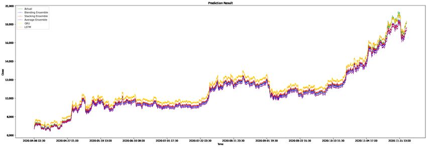
Figure 9 shows the results of the different models on the testing data. Figure 10 is
part of Figure 9, the result of stacking ensemble model is marked ‘X’ and the actual value
is marked ‘+’ to illustrate performance of models. The graph visually illustrates that the
prediction results of the stacking ensemble model are closer to the actual closing price, and
the shape of the prediction line is more identical to the shape of the actual line.Mathematics 2022, 10, 1307 14 of 21
Table 5. Results of 1-day intervals.
Price Data Price Data Price Data Price Data
Technical Indicators Sentiment Indicators Technical Indicators
Metric Model Sentiment Indicators
MAE LSTM 848.14 886.21 710.44 724.19
GRU 853.15 547.62 612.19 854.11
AE 446.10 489.68 454.78 902.65
SE 396.47 382.03 443.76 492.90
BE 395.78 359.08 461.73 521.10
MSE LSTM 1,269,660.00 1,295,847.00 1,019,135.00 1,047,841.00
GRU 1,118,205.00 428,177.66 525,815.54 911,621.13
AE 439,481.27 514,340.94 421,803.11 1,010,587.00
SE 432,656.06 253,018.37 412,734.49 392,582.15
BE 334,694.01 276,185.43 357,483.50 430,310.16
MAPE LSTM 7.05 7.45 5.81 5.92
GRU 7.27 5.26 5.87 8.34
AE 3.73 4.09 3.91 8.82
SE 3.25 3.53 3.73 4.49
BE 3.37 3.18 4.25 4.89
sMAPE LSTM 7.42 7.83 6.06 6.17
GRU 7.62 5.10 5.67 7.93
AE 3.80 4.19 3.91 8.36
SE 3.29 3.46 3.75 4.40
BE 3.44 3.16 4.16 4.74
MDA LSTM 47.21 46.35 48.50 48.93
GRU 42.49 57.94 59.23 57.51
AE 54.51 49.36 57.08 58.37
SE 54.08 59.23 56.65 57.51
BE 52.79 57.08 59.66 59.23
Figure 9. Price + technical indicator + sentiment indicator prediction results of the models.Mathematics 2022, 10, 1307 15 of 21
Table 6. Comparison of the metrics obtained by the models.
Interval 30 min 1 Day
Price Data Price Data
Technical Indicators Technical Indicators
Metric Model Sentiment Indicators Sentiment Indicators
MAE LSTM 412.554188 724.19
GRU 389.918484 854.11
AE 271.482766 902.65
SE 88.740831 492.90
BE 188.535888 521.10
MSE LSTM 184,271.5385 1,047,841.00
GRU 165,616.467 911,621.13
AE 97,194.7086 1,010,587.00
SE 30,067.70409 392,582.15
BE 58,818.47366 430,310.16
MAPE LSTM 3.966612 5.92
GRU 3.740284 8.34
AE 2.457365 8.82
SE 0.69763 4.49
BE 1.651553 4.89
sMAPE LSTM 3.884225 6.17
GRU 3.666772 7.93
AE 2.490969 8.36
SE 0.70038 4.40
BE 1.66841 4.74
MDA LSTM 51.645118 48.93
GRU 51.618368 57.51
AE 48.747214 58.37
SE 52.144449 57.51
BE 48.970129 59.23
Note: the underlined numbers indicate the best performance out of the different models.
Figure 10. Price + technical indicator + sentiment indicator prediction results of the models from 11
November 2020 to 13 November 2020.Mathematics 2022, 10, 1307 16 of 21
The second part is the comparative experiments with different data combinations. It
is shown in Table 7 that, for different time intervals, the data combinations that produce
optimal performance are not necessarily the same. Specifically, when the data interval
is one day, the combination of price data and technical indicators has better prediction
performance than other data combinations since it obtains the best value of 492.90 among
all the 1-day interval data combinations. The combination of price data, technical indicators,
and sentiment indicators outperforms the other combinations for time intervals of 30 min,
since it obtains the best value of 88.74 among all data combinations for 30-min intervals.
Table 7. Comparison of the MAE obtained by the stacking ensemble with different intervals.
Price Data Price Data Price Data Price Data
Technical Indicators Sentiment Indicators Technical Indicators
Interval Sentiment Indicators
1 day 396.47 382.03 443.76 492.90
30 min 155.933634 130.200637 107.650458 88.740831
Note: The underlined numbers indicate the best performance out of the different data combinations.
Experiments show that, in most cases, the combination of price data, technical indica-
tors and sentiment indicators outperforms the data combination in previous articles. We
can conclude that the richness of the input data used in the prediction can improve the
accuracy of the prediction.
Furthermore, other metrics are shown in Figure 11. The better the prediction obtained
with the data combination, the redder the values are; the worse the prediction obtained with
the data combination, the whiter its values are. The combination of price data and technical
indicators achieves the best performance for 1-day intervals, and the combination of price
data, technical indicators and sentiment indicators achieves the best performance for 30 min
intervals. From our experiments, we found that price data with technical indicators are
better for short-term predictions, such as predicting the next-day prices; however, price data
with sentiment indicators are better for extra-short-term predictions, such as predicting the
prices in the next 30 min.
Figure 11. Stacking ensemble model prediction results of the data combinations.
Figure 12 shows the testing data with different data combinations. Figure 13 is part of
Figure 12, the result of using all data is marked ‘X’ and the actual value is marked ‘+’ to illus-
trate performance of data combinations. The graph visually illustrates that, for the stacking
ensemble model, the accuracy of the prediction results depends on whether it is used for
short-term prediction or long-term prediction. Generally, the combination of price data and
technical indicators is better for short-term prediction, and the combination of price data,
technical indicators and sentiment indicators is better for extra short-term prediction.
At present, in the research field of Bitcoin price prediction, there are several difficulties
limiting the fair comparison of the new proposed method and previous methods: (1) the
data format is diverse and difficult to unify; (2) the data acquisition methods are different,Mathematics 2022, 10, 1307 17 of 21
and the versions are different; (3) some implementation details are not mentioned in the
theses of previous studies; (4) the source code is hard to obtain and run in new environments.
Therefore, we briefly compare the results of previous related work with our newly proposed
method in Table 8.
Figure 12. Stacking ensemble model prediction result for different data combinations.
Figure 13. Stacking ensemble model prediction result for different data combinations from 11
November 2020 to 13 November 2020.
Specially, the data combination of price and sentiment indicators under the 1-day
time internal can be considered as the variant of Li and Pan’s proposed method [1] in our
experiments. By this way, it is shown that our proposed method has got the improvement
from Li and Pan’s proposed method.
Bitcoin price data and social media text data are presented in different formats due to
different providers or acquisition tools. Most of the methods in this paper only read data in
one of the formats. For data formats other than the specified format, additional processing
work is required.
As there are no standard open data for Bitcoin price prediction, all researchers collect
data on their own. At present, there are several major trading platforms that provide their
own transaction data for Bitcoin price data. The version differences among Bitcoin’s social
media texts, such as those on Twitter or Reddit, are even more serious because the collection
tools are different and the collection times are different. For example, a tweet that wasMathematics 2022, 10, 1307 18 of 21
published yesterday may be deleted by the author today. Then, the data version collected
today is not the same as the data version collected yesterday.
Table 8. Comparison of the proposed method and previous methods in Bitcoin price prediction.
Author & Reference No. Year Method Dataset Metric
S, Ji [42] 2019 Deep neural network Daily Bitcoin price data and MAPE: 3.61%
(DNN) blockchain infomation from 29
November 2011 to 31 Decem-
ber 2018
RMSE: 197.515
S, Raju [43] 2020 LSTM (LSTM) 634 daily Bitcoin English
tweets and transaction data
from 2017 to 2018
M, Shin [29] 2021 Ensemble Minute + Transaction data from Decem- RMSE: 31.60
Hour + Day LSTM ber 2017 to November 2018 per (weighted price)
3 min
Proposed work (ensem- 2021 Stacking ensemble Tweets, transaction data, tech- MAE: 88.740831
ble deep model) deep model of 2 base nical data from September 2017 RMSE: 173.400415
models: LSTM & GRU to January 2021 per 30 min MAPE: 0.69763%
There are many parameters and implementation details in modeling and model train-
ing. In a deep neural network, the structure of each layer has many parameters. However,
these parameters are not all written in the original theses for good reasons. Moreover, there
are many details in modeling, such as the split of training and test data and some shuffle
operations to prevent overfitting of the model. These details can also be missing due to
the lengths of the theses and the focus of the topics. The lack of this information makes it
difficult to reproduce previous methods solely by the theses themselves.
If one is fortunate enough to obtain the source code with the author’s consent, there
will still be environmental and operational difficulties. We know that many machine
learning and statistical toolkits are updated very frequently. A piece of code can run under
the package version used by the author at the time, but it may not be able to run smoothly
under a new version. In addition, it is also possible that the running result is different
from the author’s result due to the inability to obtain the same running environment as
the author.
5. Conclusions
The price of Bitcoin often fluctuates wildly, inspired by the work of Li and Pan [1],
we propose an ensemble deep method, which combines two RNNs, to predict the future
price and price movement of Bitcoin based on the combination of historical transaction
data, tweet sentiment indicators and technical indicators. It is worth noting that we
crawled two datasets at different time intervals: 1 day and 30 min. Because of the financial
attribute of cryptocurrency, four evaluation indicators, the MSE, the MAE, the MAPE, and
the sMAPE, are used to measure the price prediction performance, and the movement
direction accuracy (MDA) is used to measure the price movement prediction. Two types
of comparative experiments are conducted in this research: experiments that compare
different models and experiments that compare the impact of different data combinations
on forecast prices. The results show that in the same situation, a stacking ensemble can
help with fewer training resources and better performance, and social media sentiment
analysis makes a greater contribution to extra short-term price prediction than to short-term
price prediction.
Prediction models and input data sources have great room for improvement in the
future. First, the model can be optimized from the three aspects of the model framework,
model size and optimization process to improve prediction performance [44]. For theMathematics 2022, 10, 1307 19 of 21
model framework, we can consider changing the model types and activation function. For
the model size, the width and number of hidden layers are two potential values where
we can make adjustments. For optimization, the proper setting of the hyperparameters is
essential. Second, the inclusion of other data sources may improve the existing forecasting
accuracy. In this research, we consider the historical transaction data, sentiment trends of
Twitter, and technical indicators. However, there may be other potential factors, including
regulatory and legal matters, competition between Bitcoin and other cryptocurrencies, and
the supply and demand of Bitcoin. In addition, the microexpressions of cryptocurrency
investors during trading can also be considered potential factors affecting cryptocurrency
prices. Third, we can also dynamically change the size of the window according to different
data types. For example, news is not published as quickly as social media comments, such
as tweets. Therefore, we can set different window sizes for data with different update
frequencies and study the long-term or short-term influences on prices. Experiments
based on the proposed model can be extended to research on the price prediction of other
cryptocurrencies. The new bitcoin price prediction model proposed by us provides a
reference for practitioners to avoid their potential risks in trading. In addition, researchers
can develop better regulatory measures and laws by studying the relationship 429 between
opinion analysis on social media and price movements of cryptocurrencies.
Author Contributions: Conceptualization, Y.P. and Q.J.; Data curation, Z.Y. and Y.W.; Formal analysis,
Z.Y. and Y.W.; Funding acquisition, Q.J.; Investigation, Y.P. and Q.J.; Methodology, Z.Y. and Y.P.; Project
administration, H.C., Y.P. and Q.J.; Resources, Y.P. and Q.J.; Software, Z.Y. and Y.W.; Supervision, H.C.,
Y.P. and Q.J.; Validation, Z.Y. and Y.W.; Visualization, Y.W.; Writing—original draft, Z.Y. and Y.W.;
Writing—review and editing, Z.Y., Y.W. and H.C. All authors have read and agreed to the published
version of the manuscript.
Funding: This work is supported by the Hebei Academy of Sciences under research fund No. 22602
and the National Key Research and Development Program of China under fund No. 2021YFF1200104.
Data Availability Statement: The data used in this work is available at https://github.com/Coria/
bitcoin_prediction_with_twitter, accessed on 26 February 2022.
Acknowledgments: The authors would like to thank all the anonymous reviewers for their insightful
comments and constructive suggestions that have upgraded the quality of this manuscript.
Conflicts of Interest: The authors declare that they have no known competing financial interests or
personal circumstances that could have appeared to influence the work reported in this manuscript.
References
1. Li, Y.; Pan, Y. A novel ensemble deep learning model for stock prediction based on stock prices and news. Int. J. Data Sci. Anal.
2021, 13, 139–149. [CrossRef] [PubMed]
2. Aslam, S.; Rasool, A.; Jiang, Q.; Qu, Q. LSTM based model for real-time stock market prediction on unexpected incidents. In
Proceedings of the 2021 IEEE International Conference on Real-Time Computing and Robotics (RCAR), Xining, China, 15–19 July
2021; pp. 1149–1153. [CrossRef]
3. Sutiksno, D.U.; Ahmar, A.S.; Kurniasih, N.; Susanto, E.; Leiwakabessy, A. Forecasting historical data of bitcoin using ARIMA and
α-Sutte indicator. J. Phys. Conf. Ser. 2018, 1028, 012194. [CrossRef]
4. Roy, S.; Nanjiba, S.; Chakrabarty, A. Bitcoin price forecasting using time series analysis. In Proceedings of the International
Conference of Computer and Information Technology, Dhaka, Bangladesh, 21–23 December 2018; Volume 1, pp. 1–5. [CrossRef]
5. Pant, D.R.; Neupane, P.; Poudel, A.; Pokhrel, A.K.; Lama, B.K. Recurrent neural network based bitcoin price prediction by Twitter
sentiment analysis. In Proceedings of the 2018 IEEE 3rd International Conference on Computing, Communication and Security
(ICCCS), Kathmandu, Nepal, 25–27 October 2018; Volume 1, pp. 128–132. [CrossRef]
6. Gulker, M. Bitcoin’s largest Price Changes Coincide with Major News Events about the Cryptocurrency. Available online: https:
//www.aier.org/article/bitcoins-largest-price-changes-coincide-with-major-news-events-about-the-cryptocurrency/ (accessed
on 15 December 2021).
7. Li, T.R.; Chamrajnagar, A.S.; Fong, X.R.; Rizik, N.R.; Fu, F. Sentiment-based prediction of alternative cryptocurrency price
fluctuations using gradient boosting tree model. Front. Phys. 2019, 7, 98. [CrossRef]
8. Ötürk, S.S.; Bilgiç, M.E. Twitter & Bitcoin: Are the most influential accounts really influential? Appl. Econ. Lett. 2021, 1–4.
[CrossRef]Mathematics 2022, 10, 1307 20 of 21
9. Nasekin, S.; Chen, C.Y.-H. Deep Learning-Based Cryptocurrency Sentiment Construction; SSRN Scholarly Paper ID 3310784; Social
Science Research Network: Rochester, NY, USA, 2019. [CrossRef]
10. Liu, W.; Jiang, Q.; Jiang, H.; Hu, J.; Qu, Q. A Sentiment Analysis Method Based on FinBERT-CNN for Guba Stock Forum. J. Integr.
Technol. 2022, 11, 27–39. [CrossRef]
11. Katsiampa, P. Volatility estimation for Bitcoin: A comparison of GARCH models. Econ. Lett. 2017, 158, 3–6. [CrossRef]
12. Ayaz, Z.; Fiaidhi, J.; Sabah, A.; Anwer Ansari, M. Bitcoin price prediction using ARIMA model. TechRxiv 2020. [CrossRef]
13. Bonifazi, G.; Corradini, E.; Ursino, D.; Virgili, L. A Social Network Analysis–based approach to investigate user behaviour during
a cryptocurrency speculative bubble. J. Inf. Sci. 2021.
14. Jana, R.K.; Ghosh, I.; Das, D. A differential evolution-based regression framework for forecasting Bitcoin price. Ann. Oper. Res.
2021, 306, 295–320.
15. Kim, J.M.; Cho, C.; Jun, C. Forecasting the Price of the Cryptocurrency Using Linear and Nonlinear Error Correction Model. J. Risk
Financ. Manag. 2022, 15, 74.
16. Jang, H.; Lee, J. An Empirical Study on Modeling and Prediction of Bitcoin Prices With Bayesian Neural Networks Based on
Blockchain Information. IEEE Access 2018, 6, 5427–5437. [CrossRef]
17. Mangla, N. Bitcoin price prediction using machine learning. Int. J. Inf. Comput. Sci. 2019, 6, 318–320.
18. Shen, Z.; Wan, Q.; Leatham, D.J. Bitcoin Return Volatility Forecasting: A Comparative Study of GARCH Model and Machine Learning
Model; Technical Report 290696; Agricultural and Applied Economics Association: Washington, DC, USA, 2019. Available online:
https://ideas.repec.org/p/ags/aaea19/290696.html (accessed on 15 December 2021).
19. Li, Y.; Dai, W. Bitcoin price forecasting method based on CNN-LSTM hybrid neural network model. J. Eng. 2020, 2020, 344–347.
[CrossRef]
20. Jay, P.; Kalariya, V.; Parmar, P.; Tanwar, S.; Kumar, N. Stochastic Neural Networks for Cryptocurrency Price Prediction. IEEE
Access 2020, 8, 82804–82818. [CrossRef]
21. Wołk, K. Advanced social media sentiment analysis for short-term cryptocurrency price prediction. Expert Syst. 2020, 37, e12493.
[CrossRef]
22. Jagannath, N.; Barbulescu, T.; Sallam, K.M.; Elgendi, I. A Self-Adaptive Deep Learning-Based Algorithm for Predictive Analysis of
Bitcoin Price. IEEE Access 2021, 9, 34054–34066. [CrossRef]
23. Guo, H.Z.; Zhang, D.; Liu, S.Y.; Wang, L. Bitcoin price forecasting: A perspective of underlying blockchain transactions. Decis.
Support Syst. 2021, 151, 113650. [CrossRef]
24. Loginova, E.; Tsang, W.K.; van Heijningen, G.; Kerkhove, L.; Benoit, D.F. Forecasting directional bitcoin price returns using
aspect-based sentiment analysis on online text data. Mach. Learn. 2021.
25. Sridhar, S.; Sanagavarapu, S. Multi-Head Self-Attention Transformer for Dogecoin Price Prediction. In Proceedings of the 2021
14th International Conference on Human System Interaction (HSI), Gdansk, Poland, 8–10 July 2021.
26. Parekh, R.; Patel, N.P.; Thakkar, N.; Gupta, R.; Tanwar, S. DL-GuesS: Deep Learning and Sentiment Analysis-based Cryptocurrency
Price Prediction. IEEE Access 2022, 10, 35398–35409.
27. Ibrahim, A.; Kashef, R.; Li, M.; Valencia, E.; Huang, E. Bitcoin network mechanics: Forecasting the btc closing price using vector
auto-regression models based on endogenous and exogenous feature variables. J. Risk Financ. Manag. 2020, 13, 189. [CrossRef]
28. Livieris, I.E.; Pintelas, E.; Stavroyiannis, S.; Pintelas, P. Ensemble deep learning models for forecasting cryptocurrency time-series.
Algorithms 2020, 13, 121. [CrossRef]
29. Shin, M.; Mohaisen, D.; Kim, J. Bitcoin price forecasting via ensemble-based LSTM deep learning networks. In Proceedings of the
2021 International Conference on Information Networking (ICOIN), Jeju Island, Korea, 13–16 January 2021; Volume 1, pp. 603–608.
[CrossRef]
30. Ye, Z.; Liu, W.; Jiang, Q.; Pan, Y. A cryptocurrency price prediction model based on Twitter sentiment indicators. In Proceedings of
the International Conference on Big Data and Security, Shenzhen, China, 26–28 November 2021. [CrossRef]
31. Hochreiter, S.; Schmidhuber, J. Long short-term memory. Neural Comput. 1997, 9, 1735–1780. [CrossRef] [PubMed]
32. Lipton, Z.C.; Berkowitz, J.; Elkan, C. A critical review of recurrent neural networks for sequence learning. arXiv 2015,
arXiv:1506.00019.
33. Colah Understanding LSTM Networks. 2015. Available online: http://colah.github.io/posts/2015-08-Understanding-LSTMs/
(accessed on 15 December 2021).
34. Cho, K.; van Merrienboer, B.; Bahdanau, D.; Bengio, Y. On the properties of neural machine translation: Encoder-decoder
approaches. arXiv 2014, arXiv:1409.1259.
35. Zhou, Z.-H. Ensemble Methods: Foundations and Algorithms; Chapman and Hall/CRC: London, UK, 2012. [CrossRef]
36. Dietterich, T.G. Ensemble methods in machine learning. In Multiple Classifier Systems; Springer: Berlin/Heidelberg, Germany, 2000;
pp. 1–15. [CrossRef]
37. Zhang, D.; Jiang, Q.; Li, X. Application of neural networks in financial data mining. In Proceedings of the International Conference
on Computational Intelligence, Xi’an, China, 15–19 December 2005; Volume 4.
38. Bishop, C.M. Neural Networks for Pattern Recognition; Oxford University Press: Oxford, UK, 1995.
39. Ganaie, M.A.; Hu, M.; Tanveer, M.; Suganthan, P.N. Ensemble deep learning: A review. arXiv 2021, arXiv:2104.02395
40. Goodfellow, I.; Bengio, Y.; Courville, A. Deep Learning; The MIT Press: Cambridge, UK, 2016.You can also read