Forecasting Global Weather with Graph Neural Networks - arXiv
←
→
Page content transcription
If your browser does not render page correctly, please read the page content below
Forecasting Global Weather
                                                                        with Graph Neural Networks

                                                                                            Ryan Keisler
arXiv:2202.07575v1 [physics.ao-ph] 15 Feb 2022

                                                                                        rkeisler@gmail.com

                                                                                              Abstract
                                                          We present a data-driven approach for forecasting global weather using graph
                                                          neural networks. The system learns to step forward the current 3D atmospheric
                                                          state by six hours, and multiple steps are chained together to produce skillful
                                                          forecasts going out several days into the future. The underlying model is trained
                                                          on reanalysis data from ERA5 or forecast data from GFS. Test performance on
                                                          metrics such as Z500 (geopotential height) and T 850 (temperature) improves upon
                                                          previous data-driven approaches and is comparable to operational, full-resolution,
                                                          physical models from GFS and ECMWF, at least when evaluated on 1-degree
                                                          scales and when using reanalysis initial conditions. We also show results from
                                                          connecting this data-driven model to live, operational forecasts from GFS.

                                                 1   Introduction
                                                 Numerical weather prediction (NWP), as part of the broader weather enterprise, has had an enormous
                                                 and positive impact on society. Decades of steady improvements in the quantity and types of
                                                 observational data, better modeling techniques, and more computational power have resulted in
                                                 increasingly accurate weather forecasts and growing adoption of NWP in real-world applications.
                                                 While statistical techniques have been used within NWP for decades, the core dynamical engines of
                                                 these models continue to be based on the physical principles governing the atmosphere and ocean.
                                                 More recently, spurred on by advancements in machine learning (ML), there has been a surge of
                                                 interest in statistical, data-driven techniques for weather forecasting. The motivation for using ML is
                                                 to improve upon an already extremely successful NWP program through some combination of better
                                                 forecasts, faster forecasts, or more forecasts, i.e. larger ensembles. There may also be opportunities
                                                 for using ML to advance our scientific understanding of the underlying physical processes [Cranmer
                                                 et al., 2020].
                                                 There is currently a very active hub of research at the intersection of NWP and ML. Example research
                                                 areas include: faster or more accurate solving of relevant PDEs [Bar-Sinai et al., 2019, Alieva et al.,
                                                 2021, Um et al., 2021, Li et al., 2021, Brandstetter et al., 2022], data assimilation [Frerix et al.,
                                                 2021, Maulik et al., 2021], subgrid parameterization [Brenowitz and Bretherton, 2019, Chantry et al.,
                                                 2021, Yuval et al., 2021, Meyer et al., 2021], nowcasting [Sønderby et al., 2020, Agrawal et al.,
                                                 2019, Espeholt et al., 2021, Klocek et al., 2021, Ravuri et al., 2021], nudging global NWP models
                                                 [Watt-Meyer et al., 2021], replacing global NWP models [Dueben and Bauer, 2018, Arcomano et al.,
                                                 2020, Rasp and Thuerey, 2021, Scher and Messori, 2021, Weyn et al., 2020, 2021, Clare et al., 2021],
                                                 high-level proposals for end-to-end ML weather systems [Schultz et al., 2021], and decision making
                                                 in the context of high-impact weather events [Mcgovern et al., 2017, Gagne et al., 2017].
                                                 In this work we present a data-driven, machine learning model for forecasting global weather. Our
                                                 approach is similar to and inspired by previous efforts to use ML to emulate global NWP such as
                                                 Rasp and Thuerey [2021] and Weyn et al. [2020], but with some notable differences described below.
                                                 First, we model a significantly denser physical system. Each step of our model outputs 6 physical
                                                 variables defined on 13 pressure levels on a 1.0-degree latitude/longitude grid, corresponding to
∼5,000,000 physical quantities. For reference, this is ∼50-2000X larger than the number of physical
quantities predicted by the models in Rasp and Thuerey [2021] or Weyn et al. [2020]. The motivation
for modeling a denser physical system was to reach closer towards the highly successful and much
denser physical system being modeled in traditional NWP. Put another way, our system uses ML to
perform non-linear interpolation between previously seen spatiotemporal patterns, and if the extent of
that pattern in space and time is small, then it will have simpler dynamics that are easier to interpolate
between. In the limit of using the extremely dense spatial grid and short time step used in operational
NWP simulations (well beyond the scope of this work), the ML system would "only" have to learn
the relatively compact set of physical laws driving those systems.
Second, our approach differs from Rasp and Thuerey [2021] and Weyn et al. [2020] in that we use
message-passing graph neural networks (GNNs) rather than convolutional neural networks (CNNs).
The strongest motivation for this choice was observing the success that Pfaff et al. [2021] had using
GNNs for simulating physical systems. Message-passing GNNs provide a more general architecture
than conventional CNNs, and we believe the flexibility of the underlying spatial graph provides
benefits that are well suited to NWP. These include (i) handling the spherical geometry of the earth
in a straightforward way, (ii) the potential for learning multi-resolution models, which we explored
briefly in this work, and (iii) the potential for adaptive mesh refinement, i.e. putting the compute
where it is needed at each time step, which was explored in Pfaff et al. [2021] but not in this work.
The paper is structured as follows. In Section 2 we describe the data used to train and validate our
model. In Section 3 we describe the architecture and training of our model. We cover results in
Section 4, provide additional disccusion in Section 5, and conclude in Section 6.

2     Data

We train and validate our model using one of two datasets: the ERA5 reanalysis dataset from the
European Centre for Medium-Range Weather Forecasts (ECMWF) and a subset of 2021 forecasts
from NOAA’s Global Forecast System (GFS).

2.1   ERA5

For most of the results show in this work we use the ERA5 reanalysis dataset [Hersbach et al., 2020]
from ECMWF. This dataset synthesizes decades of meteorological observations into a consistent
physical framework using 4D-Var data assimilation [Rabier et al., 2000]. The result is a set of hourly
snapshots of the 3D atmospheric state from 1950 to present.
We use six physical variables: temperature T , geopotential height Z, specific humidity Q, the eastward
component of the wind U , the northward component of the wind V , and the vertical component
of the wind W . These variables are interpolated onto a 3D grid prior to download: a 1-degree
latitude/longitude grid (horizontal resolution) and 13 pressure levels (vertical resolution). The pressure
levels are 50, 100, 150, 200, 250, 300, 400, 500, 600, 700, 850, 925, and 1000 hPa. We download
data for every third hour from 1979-01-01 to 2021-01-01. After downloading and processing data
from the Copernicus Climate Data Store, we persist the data as a single Zarr array, backed by Google
Cloud Storage, with dimensions (ntime , nlat , nlon , nvariables ∗ nlevels ) = (122728, 181, 360, 78). We
divide the data into three sets: validation (1991, 2004, 2017), testing (2012, 2016, 2020), and training
(all other years in 1979-2020, inclusive).

2.2   GFS

As discussed more in Section 4.6, we also explore training on historical forecasts from NOAA’s GFS.
We use 712 forecasts issued by GFS v16 between 2021-04-23 and 2021-10-18. We keep every third
hour of forecast output (f000, f003, etc.) from the first 249 hours of output, for a total of 59,096
individual time steps. We divide the data into a set of 18-contiguous-day chunks for training and a set
of 6-day-contiguous chunks for validation, with 3-day buffers between all chunks.
We use the same set of physical variables, the same 1-degree latitude/longitude grid, and the same
13 pressure levels that we use with ERA5. We note that, despite these similarities between our
ERA5 and GFS datasets, we do observe subtle differences between them (e.g. how variables are

                                                    2
interpolated "underground" for pressure levels that are larger than the surface pressure) that prevent
straightforward interoperability between ERA5 and GFS.

2.3        Additional Datasets

We use three additional datasets as inputs to the model. First, we use two static datasets from ERA5: a
land-sea mask and an orography dataset, both at 1-degree resolution. Additionally, we use an analytic
approximation to the top-of-atmosphere solar radiation at each location, evaluated at the current time
and 10 neighboring times spanning ± 12 hours.

3         Model

Our data-driven weather forecasting model is based on message-passing graph neural networks
(GNN) and draws heavily from the approach of Pfaff et al. [2021]. The parameters of the GNNs are
machine-learned using historical training data. We use jax and two jax-based packages: jraph for
building the graph neural network structures and haiku for managing the actual neural networks.

3.1        Architecture

The model architecture, shown in Figure 1, is made up of three components: an Encoder, a Processor,
and a Decoder. At a high level, the Encoder maps from the native data space (physical data on a
latitude/longitude grid) to an intermediate space (abstract feature data on an icosahedron grid). The
Processor then processes in that intermediate space, and the Decoder maps back to the native data
space.
The motivation to use an icosahedron grid for the intermediate representation is that it would provide
a processing grid that is more uniformly distributed and efficient than the original latitude/longitude
grid. We use the h3 package1 to define a level=2 icosahedron grid that has 5,882 nodes (compared
to 65,160 in the original lat/lon grid) with ∼3-degree (∼330 km) angular separation between nodes.
Each of the three model components is implemented as a message-passing GNN. We refer the reader
to Pfaff et al. [2021] or Battaglia et al. [2018] for more information, but in short, these GNNs are
characterized by an underlying graph (i.e. a set of nodes plus a set of directional edges connecting
some of those nodes), a neural network that updates node features, and a neural network that updates
edge features. For our neural networks we use 2-layer MLPs with ReLU activation, LayerNorm, and
256 output channels. In Figure 2 we provide a schematic view of the local graph connectivity in the
Encoder, Processor, and Decoder.

3.1.1       Encoder

As mentioned above, the Encoder maps from physical data defined on a latitude/longitude grid to
abstract latent features defined on an icosahedron grid. The Encoder GNN uses a bipartite graph
(lat/lon→icosahedron) with edges only between nodes in the lat/lon grid and nodes in the icosahedron
grid. Put another way, spatial and channel information in the local neighborhood of each icosahedron
node is gathered using connections to nearby lat/lon nodes.
The initial node features are the 78 atmospheric variables described in Section 2.1, plus solar radiation,
orography, land-sea mask, the day-of-year, sin(lat), cos(lat), sin(lon), and cos(lon). The initial
edge features are the positions of the lat/lon nodes connected to each icosahedron node. These
positions are provided in a local coordinate system that is defined relative to each icosahedron node.

3.1.2       Processor

The Processor iteratively processes the 256-channel latent feature data on the icosahedron grid using
9 rounds of message-passing GNNs. During each round, a node exchanges information with itself
and its immediate neighbors. There are residual connections between each round of processing.

      1
          https://h3geo.org/

                                                    3
Figure 1: Using the current atmospheric state, the model evolves the state forward by 6 hours. The
3D atmospheric state is defined on a uniform latitude/longitude grid, with 78 channels per pixel (6
physical variables × 13 pressure levels = 78 channels). An Encoder GNN encodes onto latent features
defined on a icosahedron grid, a Processor GNN performs additional processing of the latents, and a
Decoder GNN maps back to the atmospheric state on a latitude/longitude grid.

Figure 2: A schematic view of the local graph connectivity in the Encoder, Processor, and Decoder.
Left: local spatial and channel information is encoded into an icosahedron node using data from
nearby nodes on the input latitude/longitude grid. Center: data on the icosahedron node is further
processed using data from nearby icosahedron nodes (including itself, which is not explicitly shown).
Right: the output latitude/longitude data is created by decoding data from nearby icosahedron nodes.

3.1.3   Decoder
The Decoder maps back to physical data defined on a latitude/longitude grid. The underlying graph
is again bipartite, this time mapping icosahedron→lat/lon. The inputs to the Decoder come from
the Processor, plus a skip connection back to the original state of the 78 atmospheric variables on
the latitude/longitude grid. The output of the Decoder is the predicted 6-hour change in the 78
atmospheric variables, which is then added to the initial state to produce the new state. We found 6
hours to be a good balance between shorter time steps (simpler dynamics to model but more iterations
required during rollout) and longer time steps (fewer iterations required during rollout but modeling
more complex dynamics).

                                                 4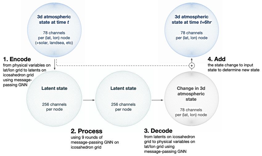
3.2     Model Size and Latency

The model has 6.7M parameters, i.e. 27 MB of information when using float32 representation. This
is ∼80,000X smaller than the 2.1 TB of ERA5 data used to train the model. As expected, we see no
evidence of overfitting on the training dataset; validation and test losses are indistinguishable from
the training loss.
The model is fast to run. After the initial overhead of loading the model weights and compiling to
XLA (all handled by jax), a single 6-hour model step takes 0.04 seconds when running on a NVIDIA
A100 GPU, i.e. creating a 5-day forecast takes 0.8 seconds.

3.3     Training

We trained our final model using the Adam optimizer and a 3-round training schedule with progres-
sively smaller learning rates: 3.5 days of training at lr=3e-4, 1 day at lr=3e-5, and 1 day at lr=3e-6.
The total training time was 5.5 days on a single NVIDIA A100 GPU, which cost approximately
$370 using the Google Cloud Platform. The training procedure used multi-resolution training data, a
multi-step loss, and a specific loss normalization, as described below.

3.3.1    Multi-resolution training data

One useful feature of using message-passing GNNs is that we can encode the relative positions
between nodes into the messages, so that a single model can learn from data at different resolutions.
We took advantage of this by first training on 2-degree data for the first round of training and then
switching to training on 1-degree data for the last two rounds. For reasons we do not understand, this
produced better results than training on 1-degree data throughout.

3.3.2    Multi-step loss

Although our core model makes a single, 6-hour step into the future, we would like it to work well
when making, say, a 5-day forecast requiring a 20-step rollout. We encouraged this behavior by
training with a multi-step loss. More specifically, during training we rolled out the model for ∼10
steps and accumulated the loss at each of those 6-hour steps. We used a progressively larger rollout
for each round of training: 4, 8, and 12-step losses, corresponding to 1, 2, and 3-day rollouts, for the
three rounds of training. Using even larger rollouts is enticing, but there are probably diminishing
returns [Metz et al., 2021], and in practice we obtained only slightly worse results when using a
4-step loss throughout.

3.3.3    Loss normalization

We observed that one of the most important choices for getting good performance was how we
normalized the data when calculating the training loss. Prior to calculating our mean-squared error
(MSE) loss, we re-scale each physical variable such that it has unit-variance in its 3-hour temporal
difference. For example, we divide the temperature data at all pressure levels by σT,3hr , where
  2
σT,3hr  is the variance of the 3-hour change in temperature, averaged across space (lat/lon + pressure
levels) and time (∼100 random temporal frames). The motivations for this choice are (i) we are
interested in predicting the dynamics of the system, so normalizing by the magnitude of the dynamics
is appropriate and (ii) a physically-meaningful unit of error, e.g. 1 K of temperature error, should
count the same whether it is happening at the lower or upper levels of the atmosphere.
We also re-scale the data by a nominal, static air density at each pressure level. This did not have a
strong impact on performance, but we did use this re-scaling in our final model.
Finally, when summing the loss across the latitude/longitude grid, we use a weight proportional to
each pixel’s area, i.e. a cos(lat) weighting.

                                                   5
Figure 3: An example of the 6-hour difference in geopotential height, temperature, and humidity in
the ERA5 dataset (left column) and the prediction from the machine learning model (right column).
The model is able to accurately predict 6-hour changes in these variables using only the initial state.
All raster figures in this paper use a 1◦ latitude/longitude grid centered on the prime meridian.
4 Results
4.1 Single-step results
Our model operates by stepping forward in 6-hour steps, and the results from an example step are
shown in Figures 3 and 4. We see that the model has learned how to use the current atmospheric state
to predict the change in that state over the next 6 hours.
4.2 Multi-step results
We can also look at how the model performs when rolled out for many steps. The process is
autoregressive: the output of the first step of the model becomes the input for the second step of the
model, and so on. In Figure 5 we show the result of a 12-step (3-day) rollout. We see that the output
of the data-driven forecast generally tracks the large-scale flows of the specific humidity at 850 hPa,
although the data-driven forecast does become smoother over time.
4.3 Stability
We observe that the model forecast is numerically stable when being rolled out ∼6 days. This is
somewhat surprising given that we did not enforce any kind of physically motivated "conservation
law" (e.g. conservation of momentum) nor did we attempt to stabilize model rollouts by training with
additional noise as in Pfaff et al. [2021].
However, we did observe hexagon-patterned instabilities beginning to form when rolling out past
∼6 days. This seems to be caused by the use of the icosahedron grid in the Processor; we did not
observe this pattern when using a simpler (but slightly less performant) architecture that did not use
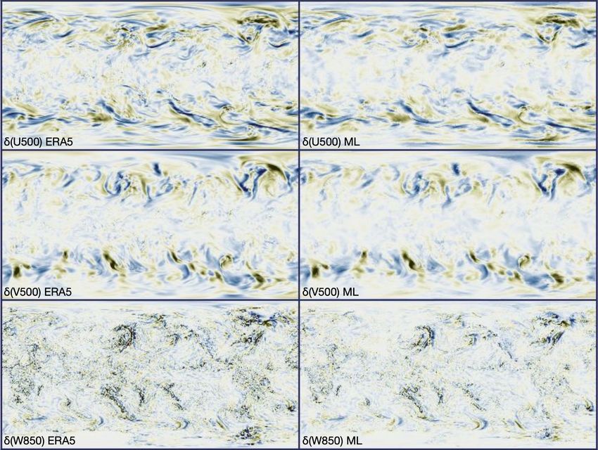
6Figure 4: An example of the 6-hour difference in eastward component of the wind, the northward component of the wind, and the vertical component of the wind in the ERA5 dataset (left column) and the prediction from the machine learning model (right column). The model is able to accurately predict 6-hour changes in these variables using only the initial state. the icosahedron grid and instead remained in latitude/longitude space. We speculate that this hexagon instability pattern would be mitigated by some combination of (i) using and predicting multiple time steps as in Weyn et al. [2020], rather than using and predicting only one time step as in this work, (ii) applying additive noise to the inputs of the model as in Pfaff et al. [2021], or (iii) mildly randomizing the graph connectivity within the icosahedron grid, a kind of edge Dropout. 4.4 Comparison to data-driven models We compare the forecast performance of our data-driven model to two previous data-driven models: Rasp and Thuerey [2021] and Weyn et al. [2020]. To the best of our knowledge, these are the two best-performing data-driven global weather forecast systems to date. The methods and discussions presented in these two papers were a major source of inspiration for the work presented here. For reference, the best-performing models in Rasp and Thuerey [2021] used a CNN to directly (i.e. not autoregressively) predict a single physical variable, like temperature at 850 hPa, at 5.625-degree resolution. Weyn et al. [2020] used a CNN to autoregressively predict four variables at ∼1.9-degree resolution: geopotential height at 500 hPa and at 1000 hPa, the 300-to700-hPa geopotential thickness, and the 2-meter temperature. The major differences between these models and ours are: (i) we use data with finer spatial resolution (1.0 deg vs 1.9 or 5.625 deg), (ii) we predict 78 channels of information rather than
Figure 5: An example multi-step rollout of the ML forecast vs reanalysis data from ERA5. Beginning
with the ERA5 initial conditions at 0 hours, the ML system steps forward autoregressively in 6-hour
steps. While the model evolves 78 separate physical channels, we show only Q850, the specific
humidity on the 850 hPa pressure level. The output of the ML forecast generally tracks the large-scale
flows seen in ERA5, although the predictions do become smoother over time. Additional media,
including videos, can be found at https://rkeisler.github.io/graph_weather

                                                  8
Figure 6: Performance metrics (RMSE of geopotential height and temperature) of our data-driven
model vs previous data-driven models from Rasp and Thuerey [2021] and Weyn et al. [2020]. The
metrics for our model are calculated on a 1.0◦ latitude/longitude grid with FWHM=1.5◦ spherical
gaussian smoothing. All metrics are computed globally (i.e. extratropics and tropics) over the year
2016.
model performance on 2016 data, and we evaluate globally (i.e. tropics + extratropics). For reasons
described in the following section, we calculate metrics for our data-driven model on a 1.0-degree
latitude/longitude grid with FWHM=1.5-degree spherical gaussian smoothing. Results are shown in
Figure 6. We see that the model presented in this work outperforms these two previous approaches,
in addition to (and perhaps due to) modeling more channels of information at higher spatial and
temporal resolution.
4.5 Comparison to operational NWP models
We compare the forecast performance of our data-driven model to two operational, physics-based
NWP models: ECMWF’s IFS and NOAA’s GFS. Below we describe some limitations of this
comparison before discussing the actual results of the comparison.
We use the 2020 performance metrics for ECMWF and GFS provided by WMO-LCDNV3 . These
metrics represent the operational, full-resolution models evaluated on a 1.5-degree latitude/longitude
grid with T120 spectral truncation. We calculate metrics for our data-driven model on a 1.0-degree
latitude/longitude grid with FWHM=1.5-degree spherical gaussian smoothing to approximate the
T120 truncation. We compute metrics for our model only over the extratropics in order to compare to
the average of the northern and southern hemisphere metrics provided by WMO-LCDNV.
It should be said that while evaluating performance metrics on these relatively coarse angular scales
is standard practice, ECMWF and GFS run simulations and provide data products at significantly
finer spatial resolution, e.g. simulations at ∼10 km horizontal resolution and data products at 0.25
degrees.
It should also be said that the performance metrics for ECMWF and GFS are evaluated as true
forecasts, while we are making our data-driven forecasts after the fact. Additionally, the initial
conditions for our data-driven model are from ERA5, a reanalysis dataset that assimilates data in
12-hour windows. This means that the initialization of a particular data-driven forecast could contain
information from 0 to 12 hours into the future. To approximately correct for this artificial advantage,
we have shifted the data-driven metrics to the left by 6 hours in Figure 7
3
https://apps.ecmwf.int/wmolcdnv/
9Figure 7: Performance metrics (RMSE of geopotential height, temperature, wind, and relative
humidity) of our data-driven model vs operational, physics-based models. The data-driven model
generally outperforms the GFS v15.2 model used in production in 2020 and generally underperforms
the ECMWF model used in production in 2020. The metrics for GFS and ECMWF are taken
from WMO-LCDNV and represent the operational, full-resolution models evaluated on a 1.5◦
latitude/longitude grid with T120 spectral truncation. The metrics for our data-driven model are
calculated on a 1.0◦ latitude/longitude grid with FWHM=1.5◦ spherical gaussian smoothing to
approximate the T120 truncation. Additionally, the metrics for our data-driven model have been
shifted to the left by 0.25 days to approximately remove the artificial advantage gained by the 0.5-
day data assimilation window of the ERA5 data used to initialize those forecasts. All metrics are
computed over the year 2020 and only over the extratropics.
With these caveats, we can see in Figure 7 that the data-driven model performs remarkably well. It
generally performs better than the GFS v15.2 model used in production in 2020 and is comparable in
performance to the ECMWF model used in production in 2020.
4.6 Connecting to live GFS runs
The work presented up to this point has focused on building and validating a data-driven weather
forecast model using historical reanalysis data from ERA5. In this section we demonstrate that
this kind of model can also be connected to a live, operational weather forecast system. The
motivations for doing this are (i) to simply demonstrate that our data-driven model can, without much
additional effort, be fused with a live system, producing a live, hybrid physics+ML system, and (ii)
to demonstrate that this system can anticipate forecast-to-forecast changes (e.g. changes between a
06Z forecast and a 12Z forecast) prior to those changes being published, which could be useful for
time-sensitive applications.
We target the operational Global Forecast System (GFS) model from NOAA, because its forecast
data is publicly and freely available. We train a model on historical GFS v16 forecasts made in April-
10Figure 8: An example of connecting our data-driven model to live data from GFS. We show forecast-to-
forecast changes in temperature (top row) and humidity (bottom row) from two sets of GFS forecasts:
the 06Z and 12Z forecasts from 2022-01-25, with the forecast valid for 2022-02-04T06:00:00. The
data-driven model (right column) was connected to the live output of these GFS forecasts and
accurately approximated the true 06Z-to-12Z change (left column) 22 minutes prior to the true change
being published.
October 2021. Our GFS-trained, data-driven model is essentially an emulator for the physics-based
GFS forecast engine. It takes as input any single GFS data snapshot, e.g. the 0-hour (f000) or the
120-hour (f120) forecast data product, and quickly (within ∼1 second) extends that forecast into the
future by some number of days. We can view the combined system as a hybrid physics+ML model,
in which the data assimilation step and the first forecast steps are performed by the physics-based
GFS model, and additional forecast steps are performed by the data-driven model.
The hybrid system works as follows. The GFS model publishes its forecast data products as usual.
We then have a simple Python script scanning for and downloading new data as it is made available.
Once a new forecast snapshot, e.g. f120, is downloaded, we preprocess it and use it to initialize a
multi-step rollout of our data-driven forecast model. The time horizon of this rollout, e.g. 3 days, is a
free parameter which can be used to balance an inherent tradeoff between wanting a longer lead time
with respect to the published data (i.e. more time to make a decision) and wanting a more accurate
approximation to the true forecast-to-forecast change (i.e. making a higher quality decision). By
repeating this process for each new forecast snapshot (f000, f003, etc.) the data-driven model is able
to "look ahead" and anticipate where the GFS forecast is heading before it gets there.
In Figure 8 we show an example of connecting our data-driven model to live GFS data. In this
example we tracked changes in temperature and humidity made between two forecasts, the 06Z and
12Z forecasts on 2022-01-25. The data-driven model was configured to extend the forecast by 3 days,
corresponding to a lead time of ∼20 minutes (because it takes GFS ∼20 minutes to publish 3 days
worth of forecast data). We see that this setting gave a high-correlation approximation to the true
forecast-to-forecast change, and, in this particular case, did so 22 minutes earlier than the relevant
12Z GFS data was published. Whether or not this level of accuracy and lead time would be useful
would depend on the actual application, but regardless, we find it interesting that the data-driven
model is able to anticipate where the physics-based model is going before it actually gets there.
5 Discussion
In this section we discuss why we believe the data-driven model described in this work performs
well, i.e. why it outperforms previous data-driven approaches and why, with the caveats described in
Section 4.5, it is comparable in performance to operational models. Our work was aimed at optimizing
forecast performance within our time and compute budget, and we did so using a large number of
11small, intuition-building experiments. As such, we did not prioritize clarity of understanding and
cannot point to a set of clean ablation studies. Nonetheless, we feel it is worthwhile to provide our
experiment-informed but somewhat subjective view of why this model performs well.
• GNNs - We have highlighted our use of message-passing graph neural networks. This
design choice was motivated by the success of Pfaff et al. [2021] in simulating physical
systems with GNNs. We have mild empirical evidence from an early experiment that the
ability to aggregate information on the sphere over a physically-uniform neighborhood (e.g.
100 km) improves upon using the latitude-dependent neighborhood of, say, a 3x3 CNN
kernel. We have not tested that the generality provided by message-passing GNNs is in itself
beneficial, but we believe it would be critical for future work such as adaptive meshing or
multi-resolution models; in these applications, a node would need to communicate to its
neighbors "here is my data" but also "here is my location".
• Simulating a dense physical system - Because traditional NWP works extremely well, we
were motivated to design a data-driven model in which key prognostic variables (temperature,
wind, etc.) are evolved forward with relatively short time steps on a relatively dense 3D
grid. As discussed below, we model a system that is denser than previous data-driven
approaches, but we note that our model is still orders of magnitude coarser than operational
NWP simulations, roughly 10X in each spatial dimension and 100X in the time step.
Here we discuss in more detail the similarities and differences between our approach and
that of Weyn et al. [2020] and Rasp and Thuerey [2021]. Like Weyn et al. [2020], we use an
iterative, auto-regressive model with 6-hour time steps, and we train with a multi-step loss,
but we model 78 physical channels (6 physical variables on 13 pressure levels) rather than
4 physical channels, and we train a ML model with 10X more parameters. Like Rasp and
Thuerey [2021], we provide ∼100 input channels (key prognostic variables defined on ∼10
pressure levels) to a ∼5M-parameter model, but we do so with significantly finer horizontal
resolution (1.0 vs 5.625 degrees) and we carry these channels forward auto-regressively
rather than directly making multi-day forecasts. The end result is that our model carries
forward ∼50-2000X more information than these previous data-driven approaches. We
believe that our decision to simulate a denser physical system was likely partially responsible
for the improvement in forecast performance that we observe relative to these approaches.
We do acknowledge that the picture is not perfectly clear. For example, with other design
choices (model size, spatial resolution, etc.) held fixed, we found that a 6-hour time step
yielded better multi-day forecast performance than a 3-hour time step, presumably because
there were twice as many error-accumulating steps during rollout in the 3-hour case.4 And
as described in Section 3.3, for reasons we do not understand, we found that an initial round
of training on coarser, 2-degree data improved the performance of our 1-degree model.
• GPU hardware and memory management - Access to a high-memory GPU and the
ability to manage its memory enabled us to push towards a larger model on a denser physical
grid. We used a 40-GB NVIDIA A100 GPU, which has significantly more memory than the
16-GB (or 32-GB) Tesla V100 used in Weyn et al. [2020] and the 11-GB GTX 2080 used in
Rasp and Thuerey [2021]. Additionally, we took advantage of the gradient "checkpointing"
(aka "rematerialization") features of jax.remat5 and hk.remat6 to reduce instantaneous
GPU memory usage and thereby compute a loss that accumulates over many rollout steps.
• Loss - There is quite a lot of freedom in how one reduces a multi-dimensional array of MSE
values (with dimensions of latitude, longitude, pressure level, physical variable, rollout time
step) to a single, scalar loss L, and thereby calculate its gradient, ∇θ L, to train the model.
When using a weighted sum over this MSE array, as we did in this work, the question
becomes, what is the relative importance of a particular physical variable, latitude range,
pressure level, etc. when it comes to the overall, long-term forecast performance? In our
experiments we found that a simple heuristic — re-scaling the data by the standard deviation
of its temporal difference, as described in Section 3.3.3 — worked significantly better than,
say, re-scaling the data by its standard deviation. As an aside we note that, while it may be
4
On the other hand, a 6-hour time step also outperformed a 12-hour time step, presumably because the
dynamics are simpler to model over the shorter 6-hour time scale. In the end we chose to use a 6-hour time step.
5
https://jax.readthedocs.io/en/latest/jax.html#jax.checkpoint
6
https://dm-haiku.readthedocs.io/en/latest/api.html#haiku.remat
12tempting to replace this heuristic with a a more end-to-end-learned approach, (i) you would
still have to use human judgement to pick a metric to optimize (e.g. globe-averaged Z500 at
a 10-day forecast horizon) and (ii) directly optimizing over tens of rollout steps might not
be effective [Metz et al., 2021], even if you are able to fit the gradient into GPU memory.
6 Conclusion
We have presented a data-driven, machine learning approach for forecasting global weather using
graph neural networks. The system uses local information to step forward the current 3D atmospheric
state by six hours, and multiple steps are chained together to produce skillful forecasts going out
several days into the future. The model works well, with forecast performance improving upon
previous data-driven approaches and comparable to operational, physical models like GFS and
ECMWF when evaluated on 1-degree scales and when using reanalysis data for the initial conditions.
We have also demonstrated that this model can be connected to live, operational forecasts from GFS
to produce a hybrid physics+ML system that anticipates the output of the physics-based GFS model.
We see several directions for future work including: (i) pushing to yet finer spatial resolution, e.g. 0.25
degrees (we have some concerns that our 1.0-degree training data contains aliased, high-frequency
information that is essentially impossible for our model to predict); (ii) using adaptive mesh refinement
to optimize forecast performance given a fixed compute budget; (iii) using this data-driven model to
cheaply generate large ensembles [Weyn et al., 2021]; (iv) creating a data-driven data assimilation
model that maps from observations to a grid of variables similar to the grid used in this work; and (v)
most ambitiously, creating an end-to-end, data-driven forecast system [Schultz et al., 2021] that maps
from observations to observations with a minimal amount of physical priors imposed. We believe
that such a system could, in principle, outperform existing physics-based forecast systems because it
could learn to predict effects that are not fully or optimally encoded into the physical models.
We believe that this work demonstrates the power of data-driven techniques for modeling the dynamics
of physical systems, and we hope that it can stimulate follow-up efforts that use machine learning in
the service of weather forecasting.
Acknowledgements
We would like to thank Stephan Rasp for valuable feedback on this work and manuscript.
References
Shreya Agrawal, Luke Barrington, Carla Bromberg, John Burge, Cenk Gazen, and Jason Hickey.
Machine learning for precipitation nowcasting from radar images, 2019.
Ayya Alieva, Dmitrii Kochkov, Jamie Alexander Smith, Michael Brenner, Qing Wang, and Stephan
Hoyer. Machine learning accelerated computational fluid dynamics. Proceedings of the National
Academy of Sciences USA, 2021.
Troy Arcomano, Istvan Szunyogh, Jaideep Pathak, Alexander Wikner, Brian R. Hunt, and Edward
Ott. A machine learning-based global atmospheric forecast model. Geophysical Research Letters,
47(9):e2020GL087776, 2020. doi: https://doi.org/10.1029/2020GL087776. URL https://
agupubs.onlinelibrary.wiley.com/doi/abs/10.1029/2020GL087776. e2020GL087776
10.1029/2020GL087776.
Yohai Bar-Sinai, Stephan Hoyer, Jason Hickey, and Michael P. Brenner. Learning data-driven
discretizations for partial differential equations. Proceedings of the National Academy of Sciences,
116(31):15344–15349, 2019. ISSN 0027-8424. doi: 10.1073/pnas.1814058116. URL https:
//www.pnas.org/content/116/31/15344.
Peter W. Battaglia, Jessica B. Hamrick, Victor Bapst, Alvaro Sanchez-Gonzalez, Vinicius Zambaldi,
Mateusz Malinowski, Andrea Tacchetti, David Raposo, Adam Santoro, Ryan Faulkner, Caglar
Gulcehre, Francis Song, Andrew Ballard, Justin Gilmer, George Dahl, Ashish Vaswani, Kelsey
Allen, Charles Nash, Victoria Langston, Chris Dyer, Nicolas Heess, Daan Wierstra, Pushmeet
13Kohli, Matt Botvinick, Oriol Vinyals, Yujia Li, and Razvan Pascanu. Relational inductive biases,
deep learning, and graph networks, 2018.
Johannes Brandstetter, Daniel Worrall, and Max Welling. Message passing neural pde solvers, 2022.
Noah D. Brenowitz and Christopher S. Bretherton. Spatially extended tests of a neural network
parametrization trained by coarse-graining. Journal of Advances in Modeling Earth Systems,
11(8):2728–2744, Aug 2019. ISSN 1942-2466. doi: 10.1029/2019ms001711. URL http:
//dx.doi.org/10.1029/2019MS001711.
Matthew Chantry, Sam Hatfield, Peter Dueben, Inna Polichtchouk, and Tim Palmer. Machine
learning emulation of gravity wave drag in numerical weather forecasting. Journal of Ad-
vances in Modeling Earth Systems, 13(7):e2021MS002477, 2021. doi: https://doi.org/10.1029/
2021MS002477. URL https://agupubs.onlinelibrary.wiley.com/doi/abs/10.1029/
2021MS002477. e2021MS002477 2021MS002477.
Mariana C.A. Clare, Omar Jamil, and Cyril J. Morcrette. Combining distribution-based neural
networks to predict weather forecast probabilities. Quarterly Journal of the Royal Meteorological
Society, 147(741):4337–4357, 2021. doi: https://doi.org/10.1002/qj.4180. URL https://rmets.
onlinelibrary.wiley.com/doi/abs/10.1002/qj.4180.
Miles Cranmer, Alvaro Sanchez-Gonzalez, Peter Battaglia, Rui Xu, Kyle Cranmer, David Spergel,
and Shirley Ho. Discovering symbolic models from deep learning with inductive biases, 2020.
P. D. Dueben and P. Bauer. Challenges and design choices for global weather and climate models
based on machine learning. Geoscientific Model Development, 11(10):3999–4009, 2018. doi: 10.
5194/gmd-11-3999-2018. URL https://gmd.copernicus.org/articles/11/3999/2018/.
Lasse Espeholt, Shreya Agrawal, Casper Sønderby, Manoj Kumar, Jonathan Heek, Carla Bromberg,
Cenk Gazen, Jason Hickey, Aaron Bell, and Nal Kalchbrenner. Skillful twelve hour precipitation
forecasts using large context neural networks, 2021.
Thomas Frerix, Dmitrii Kochkov, Jamie A. Smith, Daniel Cremers, Michael P. Brenner, and Stephan
Hoyer. Variational data assimilation with a learned inverse observation operator, 2021.
David John Gagne, Amy McGovern, Sue Ellen Haupt, Ryan A Sobash, John K Williams, and Ming
Xue. Storm-based probabilistic hail forecasting with machine learning applied to convection-
allowing ensembles. Weather and forecasting, 32(5):1819–1840, 2017.
Hans Hersbach, Bill Bell, Paul Berrisford, Shoji Hirahara, András Horányi, Joaquín Muñoz-Sabater,
Julien Nicolas, Carole Peubey, Raluca Radu, Dinand Schepers, Adrian Simmons, Cornel Soci,
Saleh Abdalla, Xavier Abellan, Gianpaolo Balsamo, Peter Bechtold, Gionata Biavati, Jean Bidlot,
Massimo Bonavita, Giovanna De Chiara, Per Dahlgren, Dick Dee, Michail Diamantakis, Rossana
Dragani, Johannes Flemming, Richard Forbes, Manuel Fuentes, Alan Geer, Leo Haimberger, Sean
Healy, Robin J. Hogan, Elías Hólm, Marta Janisková, Sarah Keeley, Patrick Laloyaux, Philippe
Lopez, Cristina Lupu, Gabor Radnoti, Patricia de Rosnay, Iryna Rozum, Freja Vamborg, Sebastien
Villaume, and Jean-Noël Thépaut. The era5 global reanalysis. Quarterly Journal of the Royal
Meteorological Society, 146(730):1999–2049, 2020. doi: https://doi.org/10.1002/qj.3803. URL
https://rmets.onlinelibrary.wiley.com/doi/abs/10.1002/qj.3803.
Sylwester Klocek, Haiyu Dong, Matthew Dixon, Panashe Kanengoni, Najeeb Kazmi, Pete Luferenko,
Zhongjian Lv, Shikhar Sharma, Jonathan Weyn, and Siqi Xiang. Ms-nowcasting: Operational
precipitation nowcasting with convolutional lstms at microsoft weather, 2021.
Zongyi Li, Nikola Kovachki, Kamyar Azizzadenesheli, Burigede Liu, Kaushik Bhattacharya, Andrew
Stuart, and Anima Anandkumar. Fourier neural operator for parametric partial differential equations,
2021.
Romit Maulik, Vishwas Rao, Jiali Wang, Gianmarco Mengaldo, Emil Constantinescu, Bethany Lusch,
Prasanna Balaprakash, Ian Foster, and Rao Kotamarthi. Efficient high-dimensional variational data
assimilation with machine-learned reduced-order models. arXiv preprint arXiv:2112.07856, 2021.
14Amy Mcgovern, Kimberly Elmore, David Gagne, Sue Haupt, Christopher Karstens, Ryan Lagerquist,
Travis Smith, and John Williams. Using artificial intelligence to improve real-time decision-
making for high-impact weather. Bulletin of the American Meteorological Society, 98, 03 2017.
doi: 10.1175/BAMS-D-16-0123.1.
Luke Metz, C Daniel Freeman, Samuel S Schoenholz, and Tal Kachman. Gradients are not all you
need. arXiv preprint arXiv:2111.05803, 2021.
David Meyer, Robin J. Hogan, Peter D. Dueben, and Shannon L. Mason. Machine learning emulation
of 3d cloud radiative effects, 2021.
Tobias Pfaff, Meire Fortunato, Alvaro Sanchez-Gonzalez, and Peter W. Battaglia. Learning mesh-
based simulation with graph networks, 2021.
F. Rabier, H. Järvinen, E. Klinker, J.-F. Mahfouf, and A. Simmons. The ecmwf operational imple-
mentation of four-dimensional variational assimilation. i: Experimental results with simplified
physics. Quarterly Journal of the Royal Meteorological Society, 126(564):1143–1170, 2000. doi:
https://doi.org/10.1002/qj.49712656415. URL https://rmets.onlinelibrary.wiley.com/
doi/abs/10.1002/qj.49712656415.
Stephan Rasp and Nils Thuerey. Data-driven medium-range weather prediction with a resnet
pretrained on climate simulations: A new model for weatherbench. Journal of Advances in
Modeling Earth Systems, 13(2):e2020MS002405, 2021.
Stephan Rasp, Peter D Dueben, Sebastian Scher, Jonathan A Weyn, Soukayna Mouatadid, and Nils
Thuerey. Weatherbench: a benchmark data set for data-driven weather forecasting. Journal of
Advances in Modeling Earth Systems, 12(11):e2020MS002203, 2020.
Suman Ravuri, Karel Lenc, Matthew Willson, Dmitry Kangin, Remi Lam, Piotr Mirowski, Megan
Fitzsimons, Maria Athanassiadou, Sheleem Kashem, Sam Madge, Rachel Prudden, Amol Mand-
hane, Aidan Clark, Andrew Brock, Karen Simonyan, Raia Hadsell, Niall Robinson, Ellen Clancy,
Alberto Arribas, and Shakir Mohamed. Skilful precipitation nowcasting using deep generative
models of radar. Nature, 597:672–677, 09 2021. doi: 10.1038/s41586-021-03854-z.
Sebastian Scher and Gabriele Messori. Spherical convolution and other forms of informed machine
learning for deep neural network based weather forecasts, 2021.
Martin Schultz, Clara Betancourt, Bing Gong, Felix Kleinert, Michael Langguth, Lukas Leufen,
Amirpasha Mozaffari, and Scarlet Stadtler. Can deep learning beat numerical weather prediction?
Philosophical Transactions of The Royal Society A Mathematical Physical and Engineering
Sciences, 379, 02 2021. doi: 10.1098/rsta.2020.0097.
Casper Kaae Sønderby, Lasse Espeholt, Jonathan Heek, Mostafa Dehghani, Avital Oliver, Tim
Salimans, Shreya Agrawal, Jason Hickey, and Nal Kalchbrenner. Metnet: A neural weather model
for precipitation forecasting, 2020.
Kiwon Um, Robert Brand, Yun, Fei, Philipp Holl, and Nils Thuerey. Solver-in-the-loop: Learning
from differentiable physics to interact with iterative pde-solvers, 2021.
Oliver Watt-Meyer, Noah D. Brenowitz, Spencer K. Clark, Brian Henn, Anna Kwa, Jeremy
McGibbon, W. Andre Perkins, and Christopher S. Bretherton. Correcting weather and cli-
mate models by machine learning nudged historical simulations. Geophysical Research Letters,
48(15):e2021GL092555, 2021. doi: https://doi.org/10.1029/2021GL092555. URL https://
agupubs.onlinelibrary.wiley.com/doi/abs/10.1029/2021GL092555. e2021GL092555
2021GL092555.
Jonathan A Weyn, Dale R Durran, and Rich Caruana. Improving data-driven global weather prediction
using deep convolutional neural networks on a cubed sphere. Journal of Advances in Modeling
Earth Systems, 12(9):e2020MS002109, 2020.
Jonathan A. Weyn, Dale R. Durran, Rich Caruana, and Nathaniel Cresswell-Clay. Sub-seasonal
forecasting with a large ensemble of deep-learning weather prediction models. Journal of Advances
in Modeling Earth Systems, 13(7), Jul 2021. ISSN 1942-2466. doi: 10.1029/2021ms002502. URL
http://dx.doi.org/10.1029/2021MS002502.
15Janni Yuval, Paul A. O’Gorman, and Chris N. Hill. Use of neural networks for stable, accurate and
physically consistent parameterization of subgrid atmospheric processes with good performance
at reduced precision. Geophysical Research Letters, 48(6):e2020GL091363, 2021. doi: https://
doi.org/10.1029/2020GL091363. URL https://agupubs.onlinelibrary.wiley.com/doi/
abs/10.1029/2020GL091363. e2020GL091363 2020GL091363.
16You can also read