A measurement-based verification framework for UK greenhouse gas emissions: an overview of the Greenhouse gAs Uk and Global Emissions (GAUGE) ...
←
→
Page content transcription
If your browser does not render page correctly, please read the page content below
Atmos. Chem. Phys., 18, 11753–11777, 2018
https://doi.org/10.5194/acp-18-11753-2018
© Author(s) 2018. This work is distributed under
the Creative Commons Attribution 4.0 License.

A measurement-based verification framework for UK greenhouse
gas emissions: an overview of the Greenhouse gAs Uk and
Global Emissions (GAUGE) project
Paul I. Palmer1 , Simon O’Doherty2 , Grant Allen3 , Keith Bower3 , Hartmut Bösch4 , Martyn P. Chipperfield5 ,
Sarah Connors7 , Sandip Dhomse6 , Liang Feng1,8 , Douglas P. Finch1 , Martin W. Gallagher3 , Emanuel Gloor6 ,
Siegfried Gonzi1,a , Neil R. P. Harris9 , Carole Helfter10 , Neil Humpage4 , Brian Kerridge11,12 , Diane Knappett11,12 ,
Roderic L. Jones7 , Michael Le Breton3,b , Mark F. Lunt2 , Alistair J. Manning13 , Stephan Matthiesen1 ,
Jennifer B. A. Muller3,c , Neil Mullinger10 , Eiko Nemitz10 , Sebastian O’Shea3 , Robert J. Parker4 , Carl J. Percival3,d ,
Joseph Pitt3 , Stuart N. Riddick7 , Matthew Rigby2 , Harjinder Sembhi4 , Richard Siddans11,12 , Robert L. Skelton7 ,
Paul Smith7,e , Hannah Sonderfeld4 , Kieran Stanley2 , Ann R. Stavert2 , Angelina Wenger2 , Emily White2 ,
Christopher Wilson5,14 , and Dickon Young2
1 School of GeoSciences, University of Edinburgh, Edinburgh, UK
2 School of Chemistry, University of Bristol, Bristol, UK
3 Centre for Atmospheric Science, The University of Manchester, Manchester, UK
4 Earth Observation Science Group, Department of Physics and Astronomy, University of Leicester, Leicester, UK
5 School of Earth and Environment, University of Leeds, Leeds, UK
6 School of Geography, University of Leeds, Leeds, UK
7 Centre for Atmospheric Science, University of Cambridge, Cambridge, UK
8 National Centre for Earth Observation, University of Edinburgh, Edinburgh, UK
9 Centre for Environmental and Agricultural Informatics, Cranfield University, Cranfield, UK
10 Centre for Ecology and Hydrology, Penicuik, UK
11 Space Science and Technology Department, Rutherford Appleton Laboratory, Oxfordshire, UK
12 National Centre for Earth Observation, Rutherford Appleton Laboratory, Oxfordshire, UK
13 Met Office, Exeter, UK
14 National Centre for Earth Observation, University of Leeds, Leeds, UK
a now at: the Met Office, Exeter, UK
b now at: Department of Chemistry & Molecular Biology, University of Gothenburg, Gothenburg, Sweden
c now at: Deutscher Wetterdienst, Meteorologisches Observatorium Hohenpeißenberg, Hohenpeißenberg, Germany
d now at: the Jet Propulsion Laboratory, Pasadena, CA, USA
e now at: Institute of Physical Chemistry Rocasolano, Madrid, Spain

Correspondence: Paul I. Palmer (paul.palmer@ed.ac.uk)

Received: 5 February 2018 – Discussion started: 16 February 2018
Revised: 15 June 2018 – Accepted: 6 July 2018 – Published: 17 August 2018

Published by Copernicus Publications on behalf of the European Geosciences Union.
11754                                                                  P. I. Palmer et al.: Quantifying UK GHG emissions

Abstract. We describe the motivation, design, and execution      1   Introduction
of the Greenhouse gAs Uk and Global Emissions (GAUGE)
project. The overarching scientific objective of GAUGE was       Human-driven emissions of carbon dioxide (CO2 ), methane
to use atmospheric data to estimate the magnitude, distribu-     (CH4 ), nitrous oxide (N2 O), and other greenhouse gases
tion, and uncertainty of the UK greenhouse gas (GHG, de-         (GHGs) to the Earth’s atmosphere perturb the balance be-
fined here as CO2 , CH4 , and N2 O) budget, 2013–2015. To        tween net incoming solar radiation and outgoing terrestrial
address this objective, we established a multi-year and inter-   radiation. These emissions, primarily from the combustion of
linked measurement and data analysis programme, building         fossil fuels and land-use-change activities, are the dominant
on an established tall-tower GHG measurement network. The        cause of the warming trend in the climate system since the
calibrated measurement network comprises ground-based,           1950s (IPCC, 2013). Minimizing the manifold impacts of in-
airborne, ship-borne, balloon-borne, and space-borne GHG         creasing atmospheric GHGs demands a structured timetable
sensors. Our choice of measurement technologies and mea-         of emission reductions. Avoiding a 2 ◦ C global temperature
surement locations reflects the heterogeneity of UK GHG          rise (Nordhaus, 1977), for which we are already close to peak
sources, which range from small point sources such as land-      emissions, requires stringent reductions that lead to zero or
fills to large, diffuse sources such as agriculture. Atmo-       negative net emissions by 2100. At the Paris Conference of
spheric mole fraction data collected at the tall towers and on   the Parties (COP) in December 2015, 195 countries agreed
the ships provide information on sub-continental fluxes, rep-    to accelerate this schedule in order to achieve net zero emis-
resenting the backbone to the GAUGE network. Additional          sions later this century. Achieving this objective demands ac-
spatial and temporal details of GHG fluxes over East An-         curate knowledge of national GHG emissions and the contri-
glia were inferred from data collected by a regional network.    butions from individual sectors. The United National Frame-
Data collected during aircraft flights were used to study the    work Convention on Climate Change (UNFCCC) requires
transport of GHGs on local and regional scales. We pur-          that all countries included in Annex 1 of that convention re-
posely integrated new sensor and platform technologies into      port their annual GHG inventory, including CO2 , CH4 , and
the GAUGE network, allowing us to lay the foundations of         N2 O. The bottom-up approach to determining these emis-
a strengthened UK capability to verify national GHG emis-        sions from individual sectors is on a production, in-use, and
sions beyond the project lifetime. For example, current satel-   disposal basis using source-dependent activity data and emis-
lites provide sparse and seasonally uneven sampling over the     sions factors. A complementary top-down approach is to ver-
UK mainly because of its geographical size and cloud cover.      ify nationwide GHG emissions using atmospheric measure-
This situation will improve with new and future satellite        ments of these GHGs, but in practice this is non-trivial and
instruments, e.g. measurements of CH4 from the TROPO-            presents many scientific challenges. Here, we describe the
spheric Monitoring Instrument (TROPOMI) aboard Sentinel-         UK Natural Environment Research Council (NERC) Green-
5P. We use global, nested, and regional atmospheric transport    house gAs Uk and Global Emissions (GAUGE) project. In
models and inverse methods to infer geographically resolved      particular, we (1) define the scientific objectives of GAUGE;
CO2 and CH4 fluxes. This multi-model approach allows us          (2) describe individual measurement types and the atmo-
to study model spread in a posteriori flux estimates. These      spheric transport models used to interpret these data; and
models are used to determine the relative importance of dif-     (3) outline the broader modelling approach that is adopted in
ferent measurements to infer the UK GHG budget. Attribut-        order to determine the magnitude and uncertainty of UK flux
ing observed GHG variations to specific sources is a major       estimates of GHGs. Throughout this paper, where relevant,
challenge. Within a UK-wide spatial context we used two          we refer the reader to peer-reviewed publications describing
approaches: (1) 114 CO2 and other relevant isotopologues         the analysis of individual GAUGE datasets.
(e.g. δ 13 CCH4 ) from collected air samples to quantify the        The UK Climate Change Act 2008 commits the UK to re-
contribution from fossil fuel combustion and other sources,      duce GHG emissions by at least 80 % below 1990 baseline
and (2) geographical separation of individual sources, e.g.      levels by 2050, with an interim target of a 34 % reduction
agriculture, using a high-density measurement network. Nei-      compared the same baseline by 2020. To establish a realis-
ther of these represents a definitive approach, but they will    tic trajectory towards the 2020 and 2050 goals, the Climate
provide invaluable information about GHG source attribu-         Change Act established five 5-year carbon budgets (2008–
tion when they are adopted as part of a more comprehen-          2032). Seven GHGs are the subject of these staged emission
sive, long-term national GHG measurement programme. We           reductions: CO2 , CH4 , N2 O, hydrofluorocarbons, perfluoro-
also conducted a number of case studies, including an instru-    carbons, sulfur hexafluoride, and nitrogen trifluoride.
mented landfill experiment that provided a test bed for new         UK government statistics report that CO2 , CH4 , and N2 O
technologies and flux estimation methods. We anticipate that     correspond to ' 81 %, 11 %, and 5 % of the UK’s esti-
results from the GAUGE project will help inform other coun-      mated 495.7 MtCO2 e (budget in 2015; Department for Busi-
tries on how to use atmospheric data to quantify their nation-   ness Energy and Industrial Strategy, 2017); the remaining
ally determined contributions to the Paris Agreement.            3 % is due to fluorinated gases. This budget, broken down
                                                                 by sector in 2015, consists of energy supply (29 %), trans-

Atmos. Chem. Phys., 18, 11753–11777, 2018                                       www.atmos-chem-phys.net/18/11753/2018/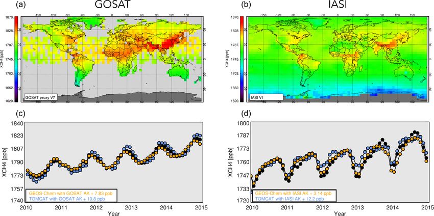
P. I. Palmer et al.: Quantifying UK GHG emissions                                                                         11755

port (24 %), business (17 %), residential (13 %), agricul-           For more than a decade the UK has included a verifica-
ture (10 %), waste management (4 %), industrial processes         tion annex chapter to its annual National Inventory Report
(2 %), and other (1 %). Emissions of CO2 are largest for          to the UNFCCC (https://www.unfccc.int, last access: 8 Au-
energy supply, transport, business, and residential sectors.      gust 2018). This chapter provides an annual comparison of
CH4 emissions are largest for agriculture and waste manage-       the reported Greenhouse Gas Inventory (GHGI) of each re-
ment, and N2 O emissions are largest for agriculture. These       ported gas to those estimated using atmospheric observa-
emission sources are very different in nature, ranging from       tions and the Bayesian inverse modelling technique InTEM
point sources (e.g. industry) to geographically large, diffuse    (Inversion Technique for Emission Modelling). The precur-
sources (e.g. agriculture). We take into account these differ-    sor to InTEM is described by Manning et al. (2011). In-
ences in the GAUGE measurement strategy, as described be-         TEM uses the output from the NAME (Numerical Atmo-
low.                                                              spheric dispersion Modelling Environment) transport model
   The primary objective of GAUGE is to quantify the mag-         (Manning et al., 2011), which describes how emissions dis-
nitude, distribution, and uncertainty of the UK GHG CO2 ,         perse and dilute in the atmosphere, and observations from the
CH4 , and N2 O budgets, 2013–2015. Our rationale is that          UK DECC (Deriving Emissions related to Climate Change)
better understanding the national GHG budget will inform          tall-tower network (described below). A recent study used
the development of effective emission reduction policies that     NAME and a hierarchical Bayesian approach to determined
help the UK to meet the interim targets of the UK Climate         UK emissions of CH4 and N2 O using the UK DECC net-
Change Act and to achieve its commitments to the Paris            work from 2012 to 2014 (Ganesan et al., 2015). They found
Agreement. To achieve our primary objective, we put to-           that a posteriori fluxes, consistent with the atmospheric mole
gether a 42-month research programme, bringing together a         fraction data, were lower than a priori values. Using geo-
purpose-built atmospheric measurement network and a range         graphical distributions of sectoral emissions, Ganesan et al.
of atmospheric transport models and inverse methods to            (2015) tentatively attributed their result to an overestimation
translate those measurements into UK GHG flux estimates.          of agricultural emissions of CH4 and a significant seasonal
More broadly, GAUGE provides an assessment of our cur-            cycle of N2 O emissions. Recent work has incorporated the
rent ability to infer GHG fluxes from atmospheric data and        reversible-jump Markov chain Monte Carlo (MCMC) inverse
strengthens the UK capability to verify national GHG bud-         modelling method (Lunt et al., 2016). The main advantage of
gets beyond the lifetime of GAUGE.                                this new approach is that the algorithm chooses the number
   GAUGE builds on a long heritage of UK atmospheric ob-          of the unknown parameters, including the geographical size
servations that have been used to estimate national GHG           of the region, to be solved given the data. A posteriori CH4
emissions. Manning et al. (2003) were the first to apply an       emissions for March 2014 inferred from the DECC network
inverse model approach to infer UK CH4 and N2 O emis-             data were consistent with Ganesan et al. (2015) (Lunt et al.,
sions, using data collected from Mace Head (MHD), Ireland,        2016). Within the GAUGE project InTEM is used together
during 1995–2000. This approach contrasted clean upwind           with other inverse methods (Sect. 3) to provide an ensem-
air that arrived from the North Atlantic with air masses that     ble of flux estimates, which provide a broader picture of the
passed over mainland UK and Europe and were influenced            range of estimates. Using InTEM also provides a link be-
by continental fluxes (Villani et al., 2010). Although these      tween GAUGE and previous UK GHG estimates.
data provided incomplete measurement coverage of the UK,             The measurement strategy we have adopted within
results using this method have been part of the UK report-        GAUGE includes long-term measurements and shorter-term,
ing to the UNFCCC. In later work, Polson et al. (2011) used       higher-resolution network measurements; focused aircraft
research aircraft observations of GHG mole fractions from         experiments; CO2 sondes; characterization of point sources
the NERC-funded AMPEP campaign (Aircraft Measurement              such as landfills; and satellite remote sensing. Our approach
of Chemical Processing and Export fluxes of Pollutants over       accounts for the heterogeneity of UK sources, e.g. point
the UK) to infer fluxes of CO2 , CH4 , and N2 O and a range       sources for power generation to large, diffuse and seasonal
of halocarbons. During AMPEP the research aircraft circum-        sources from agriculture. It also addresses the need to fo-
navigated the UK during the summer of 2005 and Septem-            cus attention on smaller regional and city scales. This fo-
ber 2006. They found that the inferred CO2 fluxes during the      cus on smaller regions will progressively grow in importance
campaign were close to the bottom-up emission inventory,          with ongoing rapid rates of urbanization across the world.
but the CH4 and N2 O fluxes were much larger than the in-         GAUGE included new in situ and remote-sensing technolo-
ventory data, albeit with significant uncertainties. The main     gies, and new measurement platforms (e.g. unmanned aerial
advantage of using an aircraft is its ability to sample nation-   vehicles, UAVs) that will help to future-proof the UK GHG
wide emissions over a relatively short time period. However       measurement network. To help attribute observed variations
limited sorties during AMPEP left gaps in sampling, which         in atmospheric GHGs to individual sources, e.g. fossil fuel
affected their ability to describe GHG emissions that include     combustion, we explored the potential of isotopologues to
large seasonal cycles (e.g. agriculture).                         chemically identify source signatures and of high-density

www.atmos-chem-phys.net/18/11753/2018/                                          Atmos. Chem. Phys., 18, 11753–11777, 2018
11756 P. I. Palmer et al.: Quantifying UK GHG emissions
2.1 In situ measurements
We use tall-tower measurements and the atmospheric base-
line observatory at MHD to provide a long-term in situ mea-
surement record to underpin the main objectives of GAUGE.
Tall towers (TTs) are used to collect atmospheric GHG mea-
surements that are sensitive to fluxes on a horizontal scale
of 10–100 s km. We also established a geographically dense
network of observations to help isolate GHG emissions from
individual sources.
Tall-tower measurement network
Figure 1. The UK DECC network funded by the UK govern-
ment (sites denoted by green triangles, 2012–ongoing), the NERC Figure 1 shows the geographical locations of the TTs that
GAUGE project (denoted by red squares, 2013–2015), and other
collect atmospheric measurements of GHGs (Tables 1 and
(blue circle). Sites are described in Table 1 and Appendix A. The
2) and provide the long-term, core measurement capability
enlarged geographical region over East Anglia shows the church
network. These sites are described in Table 4. of the UK GHG measurement network. Sampling air high
above the land surface reduces the influence of local signals
that can compromise interpretation of observed variations of
measurements to exploit geographical distributions of indi- GHGs (Gerbig et al., 2003, 2009). With the exception of the
vidual sector emissions. MHD atmospheric research station (described below) air is
Calibration activities are an integral component of typically sampled at least 50 m above the local terrain and at
GAUGE. They enable different data collected within the multiple heights (Table 1) to assess the role of atmospheric
GAUGE project to be compared and to be analysed using mixing in the planetary boundary layer.
atmospheric transport models. The use of common, interna- Tables 1 and 2 describe the five TT locations and the MHD
tionally recognized calibration scales places GAUGE data in site used in the GAUGE project. High-frequency measure-
the same framework as other international activities, includ- ments of GHGs have been collected for the past 3 decades
ing the pan-European Integrated Carbon Observing System at the MHD Northern Hemisphere background measurement
(ICOS, https://www.icos-ri.eu/, last access: 8 August 2018), station on the west coast of Ireland. They predominately
the Integrated Global Greenhouse Gas Information System represent clean western baseline conditions for the UK and
(IG3 IS, https://goo.gl/4t1x6i, last access: 8 August 2018), mainland Europe. These MHD data have been previously
and the National Oceanic & Atmospheric Administration used to infer UK-wide GHG emissions (Manning et al.,
(NOAA) Global Greenhouse Gas Reference Network run by 2011). In 2012, the UK DECC tall-tower network was es-
the Earth System Research Laboratory (ESRL). tablished across mainland UK using funding from the UK
In Sect. 2 we describe the measurements we collected dur- Department of Energy and Climate Change (with the respon-
ing GAUGE and the attributes that make them ideal for quan- sibility now residing in the Department for Business, En-
tifying nationwide GHG fluxes. We also discuss the calibra- ergy and Industrial Strategy, BEIS). Three sites were estab-
tion efforts that put these different data on internationally rec- lished (Angus, Ridge Hill, and Tacolneston; Table 1) with
ognized calibration scales, placing GAUGE data into a wider the purpose of improving the spatial and temporal distribu-
context. In Sect. 3 we describe the models we use to describe tion of measurements across the UK to reduce uncertain-
atmospheric chemistry and transport, the challenges faced, ties of GHG emissions for the devolved administrations (i.e.
and the associated inverse methods that we use to infer GHG England, Wales, Scotland, and Northern Ireland). As part of
fluxes from the GAUGE data. We conclude in Sect. 4. the GAUGE project, we augmented the UK DECC network
with two TT sites at Bilsdale and Heathfield (Fig. 1), which
started collecting data from 2013 onwards. These two new
2 Measurements sites were chosen to help fill the measurement coverage over
mid-northern England, where there is significant industrial
We present an overview of the measurements collected as
activity, and to collect measurements south of London. For
part of GAUGE in Tables 1, 2, 4, 5, and 6. We distinguish
detailed descriptions of each site, measurement and data log-
between in situ measurements, mobile measurements plat-
ging instrumentation, and the calibration protocols we refer
forms, and space-borne data. We also include a description
the reader to Appendix A; Stanley et al. (2017); and Stavert
of how we calibrate these different data.
et al. (2018) – hereafter ARS18a.
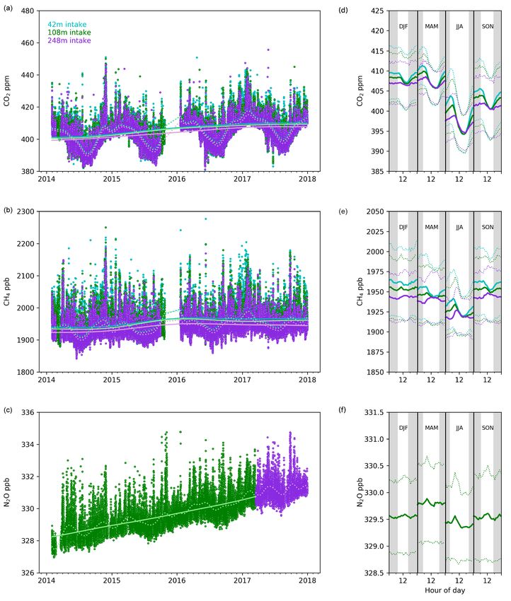
As an example, Fig. 2 shows CO2 , CH4 , and N2 O mole
fraction data from Bilsdale, North Yorkshire. Figure 2 also
shows the statistically determined baseline, long-term trend,
Atmos. Chem. Phys., 18, 11753–11777, 2018 www.atmos-chem-phys.net/18/11753/2018/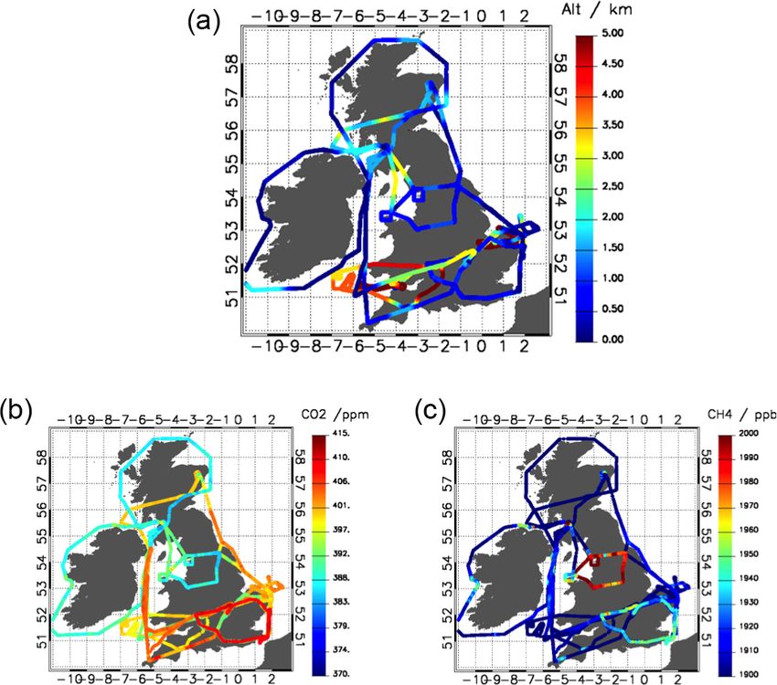
P. I. Palmer et al.: Quantifying UK GHG emissions                                                                                          11757

Table 1. The name, location, and inlet heights of the UK tall-tower network. Entries denoted by an asterisk denote an intake used by a
GC–multidetector and, if present at site, by a Medusa gas chromatograph–mass spectrometer (GC-MS).

                  Site name     Acronym      Location                 Start/end date            Altitude    Inlet heights
                                                                                               (m a.s.l.)   (m a.g.l.)
                  Mace Head     MHD          53.327◦ N 9.904◦ W       23/01/87–                         4   10*
                  Ridge Hill    RGL          51.998◦ N 2.540◦ W       23/02/11–                       204   45 & 90*
                  Tacolneston   TAC          52.518◦ N 1.139◦ E       26/07/11–                        56   54, 100* & 185
                  Angus         TTA          56.555◦ N 2.986◦ W       13/05/11–29/09/15               400   222
                  Bilsdale      BSD          54.359◦ N 1.150◦ W       30/01/14–                       380   42, 108* & 248
                  Heathfield    HFD          50.977◦ N 0.231◦ E       20/11/13–                       150   50 & 100*

Table 2. Greenhouse gas and ozone-depleting substance species and instrumentation at each UK DECC site.

      Species         MHD                     TAC                 RGL                  TTA              BIL                 HFD
      CO2             Picarro 2301            Picarro 2301        Picarro 2301         Picarro 2301     Picarro 2401        Picarro 2401
      CH4             GC-FID                  Picarro 2301        Picarro 2301         Picarro 2301     Picarro 2401        Picarro 2401
      CO              GC-RGA3                 GC-PP1              −                    −                Picarro 2401        Picarro 2401
      N2 O            GC-ECD                  GC-ECD              GC-ECD               −                GC-ECD              GC-ECD
      SF6             Medusa GC-MS            GC-ECD              GC-ECD               −                GC-ECD              GC-ECD
                                              Medusa GC-MS
      H2              GC-RGA3                 GC-PP1              −                    −                −                   −
      CRDS Nafion     Cryodried, no Nafion    Start−19/6/15       Start−6/6/15         11/1/14−end      Start−1/10/15       Start−17/6/15
      drying period

and mean diurnal cycle for each season. The statistical fitting        virtue of their age, are devoid of 14 C, which has a half-life
procedure is described in Thoning et al. (1989) and on the             of 5700 ± 30 years (Roberts and Southon, 2007). Measure-
associated NOAA/ESRL website (http://www.esrl.noaa.gov/                ments of 114 CO2 have been used extensively to determine
gmd/ccgg/mbl/crvfit/crvfit.html, last access: 8 August 2018).          ffCO2 (e.g. Meijer et al., 1996; Levin et al., 2003; Levin and
The mean Bilsdale growth rates for CO2 , CH4 , and N2 O are            Karstens, 2007; Turnbull et al., 2006, 2009; Graven et al.,
3, 8, and 0.8 ppb yr−1 , respectively. The mean seasonal am-           2009; Berhanu et al., 2017). Our sampling strategy at MHD
plitudes for these gases are 18, 51, and 0.8 ppb, respectively.        (nominally unpolluted site) and TAC (nominally polluted
Table 3 summarizes the descriptive statistics for tall-tower           site) was designed to determine the west–east gradient of
data. Diurnal variations of the atmospheric mole fractions             ffCO2 , reflecting the prevailing wind direction over the UK.
vary seasonally, particularly CO2 and CH4 that have large                  Weekly glass flask sample pairs were collected at MHD
surface fluxes. Atmospheric mole fractions of CO2 , for in-            and TAC. A commercial sampling package is used at MHD
stance, have a peak diurnal cycle of ' 10 ppm during summer            (Sherpa 60, High Precision Devices Inc., USA) as part of the
months. Diurnal variations during winter months (' 3 ppm),             NOAA Global Greenhouse Gas Reference Network global
particularly evident at lower inlet heights, provide some in-          flask sampling programme run by the Earth System Research
dication of the role of boundary layer height. Shallow win-            Laboratory (ESRL). A similar system, custom-built by the
tertime boundary layer heights that are lower than an inlet            University of Bristol, was used at TAC. Flask pairs have been
height result in measurements of free-tropospheric air that            filled at MHD for NOAA since 1991, but they have not been
is disconnected from direct surface exchange. Variations of            previously analysed for 14 CO2 . We collected and additional
CH4 are due not only to changes in anthropogenic emissions             flask from June 2014.
but also to higher summertime OH concentrations, which                     Weekly sampling commenced in June 2014 and concluded
represent the main loss term. N2 O has an atmospheric life-            in February 2016. To determine the radiocarbon CO2 con-
time ' 120 years, determined by stratospheric photolysis.              tent of our measurements, the samples are graphitized by
Our measurements show a growth rate that is consistent with            the Institute of Arctic and Alpine Research (INSTAAR) and
the global value of ' 0.9 ppb yr−1 .                                   then sent for analysis to the accelerator mass spectrome-
   We also analysed the radiocarbon content of CO2                     ter at the University of California at Irvine. Results are
(114 CO2 ) at MHD and TAC as an approach to estimate the               reported in 114 C against the NBS oxalic acid I standard
fossil fuel contribution to observed atmospheric variations            with an uncertainty of 1.8 ‰–2.5 ‰. Over the course of the
of CO2 (ffCO2 ). The underlying idea is that fossil fuels, by          GAUGE project a total of around 250 samples were anal-

www.atmos-chem-phys.net/18/11753/2018/                                                     Atmos. Chem. Phys., 18, 11753–11777, 2018
11758                                                                           P. I. Palmer et al.: Quantifying UK GHG emissions

Figure 2. (a)–(c) Hourly mean of CO2 (ppm), CH4 (ppb), and N2 O (ppb) measurements at three inlet heights (42, 108, and 248 m) at
Bilsdale, North Yorkshire, from March 2014 to July 2017 (Table 1). The statistical baseline (dashed line) and the long-term trend (solid line)
are shown in the inset for each inlet height. (d)–(f) Mean seasonal diurnal cycle for CO2 , CH4 , and CO. The dotted lines denote the ±5th
and 95th percentile. Statistical fitting procedures follow Thoning et al. (1989); further details can be found in ARS18a.

ysed for 14 CO2 . From this analysis we also received infor-             valve was used to prevent the accidental over-pressurizing of
mation about the stable isotopes 13 CO2 , CO18 O, and 13 CH4 ,           the glass flasks during flight sampling.
which we do not report here. As part of the deployment of the               A preliminary study of 14 CO2 at Tacolneston during the
Atmospheric Research Aircraft (ARA, described below) we                  GAUGE project has highlighted the benefits and difficulties
collected glass flasks for the 14 CO2 and Tedlar bags for anal-          associated with determining the fossil fuel content of CO2 in
ysis of 13 CH4 by Royal Holloway, University of London. Us-              the UK. The key outcome from the measurement programme
ing the aircraft allowed us to improve our knowledge of the              has suggested that the amount of CO2 originating from fossil
spatial gradient of these gases. Samples were taken using an             fuel burning is not significantly different from model simula-
oxygen radical absorbance capacity (ORAC) metal bellows                  tions using Emission Database for Global Atmospheric Re-
pump, fitted with a pressure relief valve. For the glass flask           search (EDGAR) emissions. However, there were a number
sampling an adapter containing a downstream pressure relief              of difficulties associated with making these measurements.
                                                                         First, we used a number of assumptions and data corrections

Atmos. Chem. Phys., 18, 11753–11777, 2018                                                  www.atmos-chem-phys.net/18/11753/2018/
P. I. Palmer et al.: Quantifying UK GHG emissions 11759
Table 3. Mean seasonal amplitude and mean growth rates of CO2 , regional network of five sensors over East Anglia (Fig. 1, Ta-
CH4 , and N2 O at the Bilsdale (BSD), Heathfield (HFD), Ridge Hill ble 4), where there is a high density of crop agriculture, a sec-
(RGL), Tacolneston (TAC), and Angus (TTA) tall-tower sites. The tor with large seasonal emissions of CH4 and N2 O attributed
mean seasonal amplitude (±1 standard deviation) was calculated to fertilizer application (Sect. 1). Developing this regional
from the annual peak-to-peak amplitudes. The mean growth rate is network supports the inference of higher-resolution emission
the average of the first derivative of the statistical long-term trend.
estimates (Manning et al., 2011). We used data from this
network to determine how well we can distinguish between
Site Intake Mean seasonal Mean growth
sources of CH4 that range from spatially diffuse agricultural
height (m) amplitude (ppm) rate (ppm yr−1 )
sources to point sources such as landfills.
42 18 ± 2 3 We purposely distributed the network across East An-
BSD 108 18 ± 1 3 glia (Fig. 1), comprising one atmospheric observatory (Wey-
248 18 ± 1 3
bourne) and three churches (Holy Trinity, Haddenham; All
50 11 ± 6 3 Saints, Tilney; and St Nicholas, Glatton), and one wind tur-
HFD
100 13 ± 5 3 bine (Earl’s Hall). East Anglia is one of several dense regions
CO2
45 16 ± 2 3 of UK agriculture. It was chosen for two reasons: (1) there is
RGL
90 17 ± 2 3 little variation in terrain height, simplifying boundary layer
54 17 ± 2 3 transport and mixing, and (2) all sites are within an hour of
TAC 100 18 ± 2 3 Cambridge, simplifying logistics associated with maintain-
185 18 ± 2 2 ing long-term sites. Additional criteria for site selection in-
TTA 222 16 ± 1 2 cluded sufficient sampling height (15–50 m for the East An-
glia network, Table 4), remoteness from very local sources
42 57 ± 7 8 of CH4 , easy accessibility for maintenance, and low running
BSD 108 56 ± 2 8
248 41 ± 4 7
costs.
Figure 3 shows that the CH4 mole fraction data collected
50 70 ± 40 6 from the three churches exhibit similar variations on diurnal,
HFD
100 60 ± 10 7
CH4 daily, and monthly timescales, suggesting that the surround-
RGL
45 70 ± 20 8 ing villages have similar sources and/or at least some of the
90 60 ± 10 8 observed variation reflect larger-scale variations. Observed
54 70 ± 20 9 sub-annual variations of CH4 at the Weybourne Atmospheric
TAC 100 70 ± 20 9 Observatory (WAO), for different years, are comparable to
185 60 ± 10 8 those at inland sites on seasonal timescales but are muted on
TTA 222 31 ± 9 13 faster timescales because it mainly observes clean upwind
air. The shape of the diurnal cycle at the church sites sug-
BSD 108 0.8 ± 0.3 0.8
HFD 100 1.0 ± 0.4 0.9
gests that the boundary layer height likely plays the dominant
N2 O role. Seasonal variations reflect changes in regional sources,
RGL 90 1.2 ± 0.3 0.9
TAC 100 0.6 ± 0.3 1.0 boundary layer variations, and the OH sink.
Using the NAME-InTEM inverse model framework (Man-
ning et al., 2011), we used the East Anglian network to infer
to account for terrestrial biosphere fluxes and nuclear emis- county-level CH4 fluxes for Cambridgeshire, Norfolk, and
sions. For nuclear emissions, we expect that the applied cor- Suffolk. Our a posteriori fluxes were consistent with those
rection can be significantly improved by provision of higher- from the UK National Atmospheric Emissions Inventory
frequency emissions data from the nuclear industry. Second, (Connors et al., 2018). For this work it was difficult to accu-
the location of the sampling site, and timing and frequency of rately estimate associated uncertainties because of difficul-
measurements are paramount in determining a strong enough ties associated with defining the “background” CH4 entering
14 CO signal from fossil fuels to distinguish it from the back- into the small, regional domain chosen. This difficulty will be
2
ground uncertainty. Many lessons were learnt in the GAUGE avoided when these data are included in larger, regional-scale
project that will allow for an improved and more robust sam- inversions. We find that regional networks, embedded within
pling strategy to be applied to future measurements (Wenger a nationwide network, show great potential for revealing ad-
et al., 2018). ditional spatial and temporal details of emissions such as
point source emissions from landfills (Riddick et al., 2017).
East Anglian church network Such a regional network would best serve a national-scale
network over regions where a priori emission uncertainties
A key objective of GAUGE was to improve understanding are largest.
of how to attribute observed variations of GHGs to particu-
lar sectors. To help address that objective, we established a
www.atmos-chem-phys.net/18/11753/2018/ Atmos. Chem. Phys., 18, 11753–11777, 201811760 P. I. Palmer et al.: Quantifying UK GHG emissions
Table 4. Details of the measurements made in the GAUGE East Anglian network.
Site Lat [◦ N], long [◦ E] Site elevation Inlet height Start End Measurements Compounds Institute lead
[m] [m]
Haddenham (HAD) 52.359, 0.148 40 25 07/2012 Ongoing GC-FID CH4 UCAM
Weybourne (WEY) 52.950, 1.122 15 15 02/2013 Ongoing GC-FID CH4 , N2 O UCAM/UEA
Tilney (TIL) 52.737, 0.321 6 25 06/2013 Ongoing GC-FID CH4 UCAM
Glatton (GLA) 52.461,-0.304 28 20 10/2014 04/2016 In situ FTIR CH4 , CO2 , N2 O, CO ULeic
Earls Hall (ELH) 51.813, 1.118 17 50 11/2014 12/2015 CRDS/QCL CH4 , CO2 , N2 O UCAM
Figure 3. Observed variations of CH4 mole fraction data collected at one atmospheric observatory (Weybourne, WAO, 13 February 2013–6
May 2014) and three church steeples at Haddenham (HAD, 3 July 2012–23 September 2015), Tilney (TIL, 7 June 2013–31 August 2015),
and Glatton (GLA, 22 October 2014–5 April 2016). The coloured envelope denotes the 95 % confidence interval of the hourly, daily, and
monthly mean.
2.2 Mobile GHG measurement platforms 2.2.1 North Sea ferry
We use mobile platforms to help integrate measurements that We installed an 8 ft. air-conditioned sea container on
are sensitive to different spatial scales. The two principal the Rosyth (56.02262◦ N, 3.43913◦ W)-to-Zeebrugge
platforms we use are the Rosyth–Zeebrugge North Sea ferry (51.35454◦ N, 3.175863◦ E) ferry operated by DFDS
and the British Aerospace 146 (BAe-146) Atmospheric Re- Seaways. The container includes a Picarro 1301 cavity
search Aircraft. We also describe the deployment of balloon- ring-down spectrometer (CRDS) to measure mole fractions
borne sensors and a fixed-wing UAV, as examples of GAUGE of CH4 , CO2 , and H2 O. This ship of opportunity completes
fostering new atmospheric GHG measurement technology. three return journeys per week, traversing the North Sea
In the conventional sense, a mobile measurement platform is at different times of day, thereby minimizing temporal
one that is fixed in one place for some length of time but is measurement bias, which can sometimes complicate the
sufficiently mobile that it can be moved elsewhere to con- analysis of data from mobile platforms. The prevailing
tinue measurements. The ferry platform can be considered a winds over the North Sea are westerly and southwesterly,
continually moving mobile platform. so that measurements frequently sample the outflow from
the UK, and also allow us to distinguish between UK and
mainland European emissions.
Atmos. Chem. Phys., 18, 11753–11777, 2018 www.atmos-chem-phys.net/18/11753/2018/P. I. Palmer et al.: Quantifying UK GHG emissions 11761
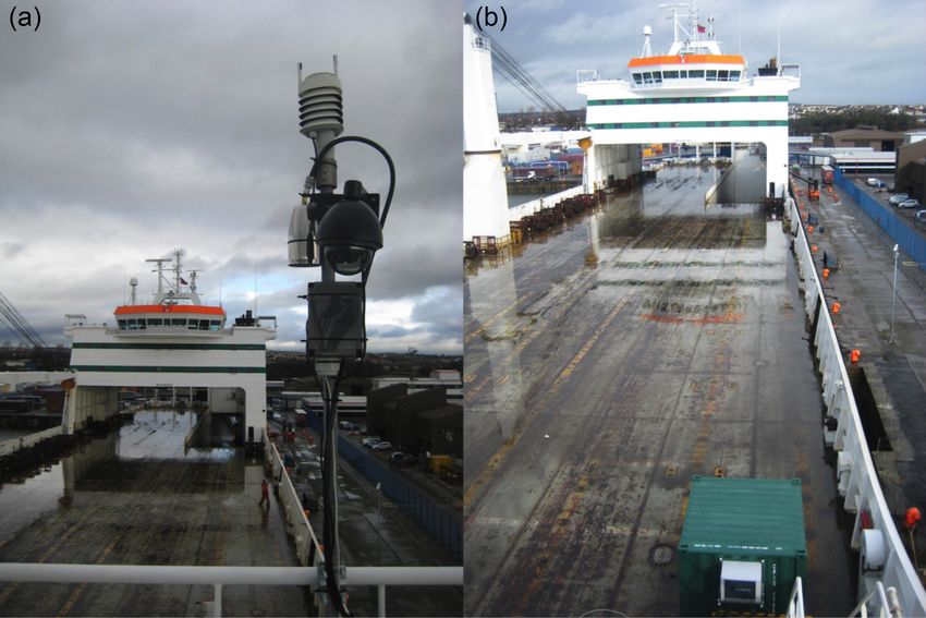
Figure 4. Photos of the North Sea ferry mobile GHG laboratory on
the DFDS Seaways Longstone (now the F innmerchant). View of
the (a) weather station mounted on the top deck and (b) from the
air inlet mounted on top of the mobile laboratory located on the
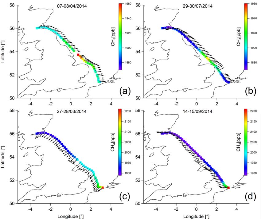
weather deck. Figure 5. Observed temporal and spatial variations in CH4 mole
fractions along the route of the DFDS freight ferry in March, April,
July, and August 2014. Arrows denote local wind direction.
Figure 4 shows the view from the mobile laboratory, with
sample inlets located at the bow away from local sources
on the ferry (chimney stacks towards the stern). The ini- ing the ARA include (1) collecting a snapshot of precise and
tial installation was on 25 February 2014 on DFDS Sea- traceable GHG concentration distributions over and around
ways Longstone (now the F innmerchant) and ran until the UK; (2) integrating atmospheric GHG information col-
15 April 2014. A weather station (Vaisala WXT 520) located lected by tall towers, ferry transects, and space-borne instru-
on the top deck provides basic meteorological data (air tem- ments; (3) defining and executing sampling experiments to
perature, pressure, wind speed and direction); geolocation in- enable measurement-led quantification of GHG fluxes at the
formation (latitude, longitude, ship speed, course) is obtained regional scale (O(100 km)); and (4) defining and executing
from a Garmin GPS unit fixed to the roof of the sea container. sampling experiments to challenge Earth system models and
Figure 5 shows example CH4 data for sailings in March, inversion models in terms of better understanding model at-
April, July, and September 2014, which shows a dynamic mospheric transport error and surface emission distribution.
range that reflects geographical variations in sources. Differ- The ARA is a BAe-146-301 aircraft that has been con-
ences between individual sailings reflect changes in seasonal verted to a mobile laboratory, including a variety of forward-
emissions and prevailing meteorology. Figure 5 shows in- and backward-facing external inlets so that air can be sam-
stances when observed values are influenced by emissions pled by instruments within the main cabin. It also includes
from the UK and the North Atlantic background during a number of ports that can host remote-sensing instruments.
spring and summer (Fig. 5a, b), and when observed values Table 5 describes the instruments that we deployed during
are influenced by high emissions from Germany and central GAUGE, including in particular instruments that measure
Europe (Fig. 5c) and by lower emissions from Scandinavia CO2 , CH4 , and N2 O, and a small complementary suite of
(Fig. 5d). To avoid contamination from GHG emissions on other trace gases and thermodynamic parameters. We made
board the ship (e.g. engine emissions, venting of the below- continuous measurements of CO2 and CH4 at a frequency
deck cargo area), individual data points were removed when of 1 Hz using a Fast Greenhouse Gas Analyzer (FGGA, Los
the ship was in port or when the wind blew from the direction Gatos, USA). For a detailed description of the FGGA – in-
of the chimney stacks. A more detailed description of the in- cluding its operating principles, data processing, and calibra-
struments and the data interpretation can be found in Helfter tion – we refer the reader to O’Shea et al. (2013). We also
et al. (2018). collect 1 Hz measurements of N2 O and CH4 from a quantum
cascade laser absorption spectrometer (Aerodyne Research
2.2.2 BAe-146 Atmospheric Research Aircraft Inc., USA). Further details of the instrument are described
by Pitt et al. (2016). We use the Met Office Airborne Re-
We use the NERC/Met Office Atmospheric Research Air- search Interferometer Evaluation System (ARIES), a Fourier
craft (ARA), operated by AirTask Group Ltd, to provide transform infrared spectrometer (FTIR), to retrieve partial
vertical profile distributions of atmospheric GHGs over and columns of CH4 and CO2 and vertical profiles of H2 O and
around the British Isles. The specific objectives of deploy- temperature. Further details about ARIES can be found in
www.atmos-chem-phys.net/18/11753/2018/ Atmos. Chem. Phys., 18, 11753–11777, 201811762 P. I. Palmer et al.: Quantifying UK GHG emissions
Allen et al. (2014). Other instruments listed in Table 5 are
core ARA science instruments, which are described in Allen
et al. (2011) and references therein.
During GAUGE we conducted a total of 16 individual
flight sorties over/around mainland UK and Ireland between
May 2014 and March 2016, comprising over 65 h of atmo-
spheric sampling. These flights are summarized in Table 6
and Fig. 6. A typical flight sortie coordinated upwind and
downwind sampling of a target flux region (e.g. the London
metropolitan area), based on the prevailing boundary layer
wind direction, to attempt sampling of air masses that have
been impacted by regions with GHG emissions and uptake.
We also designed flights to sample outflow from mainland
UK and continental Europe, and outflow from the Irish and
North seas on days with strong westerly flow regimes (e.g.
Pitt et al., 2018).
To capture regional emissions during GAUGE, we col-
lected measurements that were mostly in the boundary layer,
as defined by in-flight thermodynamic profiling, which was
typically below 2 km altitude. Occasionally, to characterize Figure 6. Flight tracks for all FAAM flights during GAUGE from
long-range transport of pollutants into our study region, we 15 May 2014 to 4 April 2016 (Table 6). Colours denote (a) altitude,
collected measurements during deeper vertical profiles into (b) CO2 mole fraction, and (c) CH4 mole fraction.
the free and upper troposphere. Other flight profiles included
surveys around Britain and Ireland and flying around tall
towers, as described below. of ' 35 km. A typical flight is 3–4 h, including rapid descent
Figure 6 shows a summary plot of the CO2 and CH4 data of 20–30 mins. The system used during GAUGE is expend-
collected during GAUGE. In particular, it illustrates the hor- able but could be easily recycled with the installation of an
izontal and vertical spatial coverage of the aircraft sampling onboard GPS sensor.
and the dynamic range of mole fractions sampled. These ob- Figure 7 shows preliminary data from two ChemSonde
served variations are due to differences in flight altitude and launches from WAO on 14 April 2016 to test the viabil-
the time of year of the superimposed flights (Table 6), dif- ity of the system. Met Office surface analysis charts (not
ferences in air mass history, and the spatial and temporal shown) indicate that the UK was under the influence of a
variability of local and regional fluxes across seasons and low-pressure anticyclone in the North Atlantic, transporting
sources. moist air over the southern half of the UK, during the pe-
riod of measurements. A low-level stratus cloud deck, with
2.2.3 Balloon CO2 sondes drizzle, and low SW winds predominated over WAO during
the morning of 14 April, with light winds and steady rain
Balloons offer an alternative platform for the collection of during the afternoon. The first instrument was launched at
vertical profiles of GHGs, building on the approaches used 10:39 UTC, and the second at 14:30 UTC. For brevity, we
widely by the meteorological and stratospheric communi- only show data to 10 km. The sharp decrease in CO2 from
ties. Here, we describe some of the first balloon launches of near-surface altitudes to ' 1 km during the morning launch
small-scale CO2 sensor technology that have been adapted and the increase in boundary layer CO2 concentrations from
for atmospheric sciences as part of a collaboration between morning to afternoon launches suggest some local influence.
the University of Cambridge, SenseAir (Sweden, https:// We also noticed that some small-scale increases in CO2 (1.8
senseair.com/, last access: 8 August 2018), and Vaisala (Fin- and 7.5 km from the morning launch and 2.5 km from the
land). The instrument consists of a small, sensitive nondis- afternoon launch) correspond to increased relativity humid-
persive infrared (NDIR) CO2 sensor developed by SenseAir. ity, indicating possible cloud layers. NOAA HYSPLIT 48 h
The instrument sampling is 1 Hz with data transmitted to the back trajectories (Stein et al., 2015) initialized at these lower
Vaisala MW41 ground station via a Vaisala RS41 radiosonde. and mid-troposphere altitudes (not shown) indicate that we
The corresponding vertical resolution of the collected data is are sampling background maritime air over the North At-
4–5 m. The dimensions and weight of the instrument pack- lantic that has been lofted prior to interaction with land sur-
age are approximately 150 × 150 × 300 mm and 1 kg, respec- faces. Differences in relative humidity close to 6 km suggest
tively. Heavy-duty cable ties are used to seal the enclosure that the morning cloud structure has been dissipated by the
and secure the radiosonde to the outside. A 1200 g balloon stronger afternoon winds. We attribute the 4–5 ppm differ-
(TOTEX, Japan) is used for lifting the payload up to a ceiling ence between CO2 instruments above 6.5 km to problems
Atmos. Chem. Phys., 18, 11753–11777, 2018 www.atmos-chem-phys.net/18/11753/2018/P. I. Palmer et al.: Quantifying UK GHG emissions 11763
Table 5. Key instrumentation on board the FAAM aircraft for GAUGE-specific flights, including measurement principles and references to
instrument characteristics (where available). VUV denotes vacuum ultraviolet (light); HFCs, PFCs, and VOCs denote hydrofluorocarbon,
perfluorocarbons, and volatile organic compounds, respectively; and PRT denotes platinum resistance thermometer.
Parameter Technique Manufacturer/model Reference
CO VUV fluorescence Aerolaser, AL5002 Gerbig et al. (1999)
O3 UV absorption Thermo Electron Corporation, 49C
CH4 , CO2 Off axis-integrated cavity Los Gatos, FGGA 907-0010 O’Shea et al. (2013)
Output spectroscopy
N2 O, CH4 Tunable infrared laser Aerodyne Research, QC-TILDAS-CS Pitt et al. (2016)
Differential absorption spectroscopy
NOx Chemiluminescence Air Quality Design Di Carlo et al. (2013)
HFCs, PFCs, SF6 , C2 –C7 VOCs Whole-air sampling Thames Restek Lewis et al. (2013)
114 CO2 Glass flask sampling NORMAG
δ 13 CH4 Tedlar bag sampling SKC
CO2 , CH4 , O3 , H2 O, CO FTIR total column remote sensing UK Met Office, ARIES Allen et al. (2014)
Humidity Chilled mirror General Eastern, GE 1011B Ström et al. (1994)
Temperature PRT Rosemount Aerospace, 102 AL Petersen and Renfrew (2009)
Wind vector 5-hole probe BAE Systems & UK Met Office Brown et al. (1983)
with the zero baseline drift and to a faulty span measurement ventional walkover flux surveys were conducted by GGS,
during the afternoon pre-launch preparation. Further studies and dynamic automated flux chambers were operated on the
with ChemSonde are planned, with emphasis on improving flanks of the capped landfill area to investigate seeps under
design, operation, and post-processing of data. the capped area where this met an active cell. Tracer releases
of perfluorocarbon and acetylene were also conducted from
2.2.4 Unmanned aerial vehicles for hotspot various key points across the site to allow proxy flux calcula-
measurement campaign tions from mobile (public road) plume sampling downwind.
Specific experiments and instrument siting were designed on
UAVs represent a new atmospheric measurement platform each day of the intensive period in response to weather (es-
for studying atmospheric GHGs. They can be deployed pecially wind) conditions to characterize inflow and outflow
rapidly to provide vertical information across a horizonal di- from different areas of the site. We deployed a fixed-wing
mension O(100 m). Within GAUGE, researchers used a va- UAV equipped with a CO2 NDIR sensor around the site (Ed-
riety of measurement technologies, including fixed-wing and inburgh Instruments Gascard NG). We also launched a teth-
rotary UAVs, to develop and refine new methods to use at- ered rotary UAV, which sampled air up to 120 m above the
mospheric measurements to quantify CH4 and CO2 emission local terrain. This air was analysed using a ground-based in-
from a landfill site (Riddick et al., 2016, 2017; Sonderfeld strument (Los Gatos Research Ultraportable Greenhouse Gas
et al., 2017; Allen et al., 2018a). This represents one of the Analyzer) via a 150 m length of Teflon tube. This configura-
first demonstrations of using UAVs to sample GHG emis- tion allowed us to sample vertical profiles of CH4 and CO2
sions. The reader is referred to Allen (2014) and Allen et al. over the landfill site.
(2015) for further details of the underlying technology. We also established a fixed-site monitoring station mea-
We conducted a 2-week measurement campaign at a land- suring CO2 and CH4 mole fractions to put the campaign into
fill site near Ipswich, England (operated by Viridor Ltd), in a longer temporal context, to help test plume inversion tech-
August 2014. This campaign brought together researchers niques, and to test the efficacy of continuous in situ moni-
from the University of Bristol, University of Cambridge, toring to generate flux climatologies (Riddick et al., 2016,
Denmark Technical University, University of Edinburgh, 2017). Sonderfeld et al. (2017) demonstrate how to combine
University of Leicester, University of Manchester, Royal a computational fluid dynamics model (which accounts for
Holloway University of London, University of Southamp- topographical data from a 3-D lidar survey data) with contin-
ton, and Ground Gas Solutions (GGS) Ltd. The landfill in- uous in situ FTIR measurements to infer and apportion fluxes
cludes historic, capped and active, and open landfill cells; a across the surface area of the landfill site. They showed in
leachate plant; a gas collection network; and a gas-burning particular the ability of this approach to distinguish between
energy generation facility. individual emission regions within a landfill site, allowing
We equipped the site with a 20 m eddy covariance flux better source apportionment compared with other methods
tower, three Los Gatos Research Ultraportable Greenhouse that derive bulk emissions.
Gas (CO2 and CH4 ) Analyzers (triangulated across the Our UAV deployment during this experiment has since led
capped and open cell areas), a closed-path FTIR, and five 3-D to further refinements to the method and platform, and to our
sonic anemometers to characterize flow over the site. Con-
www.atmos-chem-phys.net/18/11753/2018/ Atmos. Chem. Phys., 18, 11753–11777, 201811764 P. I. Palmer et al.: Quantifying UK GHG emissions
(a) CO2 concentration (b) Relative humidity
10 000 10 000
7500 7500
5000 5000
Height above sea level in metres 2500 2500
0 0
390 400 410 0 25 50 75 100
Concentration (ppm) RH %
(c) Wind direction (d) Wind speed
10 000 10 000
7500 7500
5000 5000
2500 2500
0 0
0 100 200 300 5 10 15 20
Direction (degrees) Speed (m s -1 )
Figure 7. Preliminary balloon-borne CO2 data launched on 14 April 2016 from Weybourne Atmospheric Observatory, UK (Fig. 1). Correl-
ative measurements of (b) relative humidity, (c) wind speed, and (d) wind direction are also shown. Data are averaged every 10 s. Red ticks
denote the morning launch, and black ticks denote the afternoon launch.
use of similar technology to infer fluxes from other UK land- servation (TANSO) Fourier transform spectrometer (FTS),
fills (Allen et al., 2018a). A recent validation of a new mass which observes atmospheric spectra, and the Cloud and
balancing algorithm based on tethered UAV sampling of a Aerosol Imager (CAI), which provides multi-spectral im-
known CH4 release rate demonstrated that a 20 min flight on agery and coincident cloud and aerosol information (Kuze
a single rotary UAV flight can reproduce the known release et al., 2009). TANSO-FTS has a ground footprint of approx-
rate with an mean accuracy of 14 % and an (1σ ) uncertainty imately 10.5 km2 and returns to the same point every 3 days.
of < 40 % (Allen et al., 2018b). Collectively, these measure- For illustration, we show GOSAT SWIR dry-air column-
ments allowed us to test and compare a wide range of estab- averaged CH4 mole fractions that are inferred from version
lished and novel sampling technologies and flux quantifica- 7.0 of the proxy retrieval developed by the University of Le-
tion approaches. It also allowed us to examine how to op- icester (Sect. 3). These data are sensitive to changes in at-
timize different combinations of data to determine net bulk mospheric CH4 in the lower troposphere. The proxy retrieval
(whole-site) GHG fluxes. method simultaneously fits CH4 and CO2 spectral features
in nearby wavelengths. The underlying idea is that taking the
2.3 Space-borne observations of GHGs ratio of the CH4 and CO2 fitted in nearby wavelength regions
effectively removes spectral artefacts common to both CH4
Satellites provide global, near-continuous, and multi-year and CO2 (e.g. scattering). The conventional method of using
measurements of GHGs that are used to infer GHG fluxes these data is to multiply the ratio by model CO2 , assuming
on sub-continental scales and to provide boundary conditions that CO2 varies in space and time less than CH4 . The result-
for regional atmospheric transport models. Within GAUGE, ing proxy XCH4 data have been evaluated extensively using
we explore the potential of short-wave infrared (SWIR) col- data from the Total Carbon Observing Network (Parker et al.,
umn measurements of CO2 and CH4 from the Japanese 2011, 2015).
Greenhouse Gases Observing SATellite (GOSAT) and ther- IASI is one of a series of FTS instruments on the polar-
mal IR column measurements of CH4 from the European In- orbiting meteorological MetOp platforms (Hilton et al.,
frared Atmospheric Sounding Interferometer (IASI). For the 2012) designed primarily for operational meteorology. There
sake of brevity, we describe here only the pertinent details of are two IASI instruments currently operating: MetOp-A was
GOSAT and IASI and refer the reader to other studies ded- launched on 19 October 2006, and MetOp-B was launched
icated to these satellite instruments (e.g. Kuze et al., 2009; on 17 September 2012. IASI has an across-track measure-
Clerbaux et al., 2009). ment swath of 2200 km, resulting in near-global coverage
GOSAT is the first space-borne mission dedicated to mea- twice a day with a local solar overpass time of 09:30 and
suring GHGs. It was launched in a sun-synchronous orbit 21:30. It measures three spectral bands that span a range
with a local overpass time of 13:00 by the Japanese Space of thermal IR wavelengths from 4 to 15.5 µm (Clerbaux
Agency (JAXA) in January 2009 (Kuze et al., 2009). We et al., 2009), which are most sensitive to CH4 in the mid-
use the Thermal And Near-infrared Sensor for carbon Ob-
Atmos. Chem. Phys., 18, 11753–11777, 2018 www.atmos-chem-phys.net/18/11753/2018/P. I. Palmer et al.: Quantifying UK GHG emissions 11765
Table 6. Diary of FAAM survey flights for GAUGE between May 2015 and March 2016, including take-off and landing times, sampling
locations, and a brief description of mission profiles.
Flight No. Date Take-off (UTC) Landing (UTC) Description
B848 15/05/14 12:07:07 16:46:25 North Sea Gas Rigs (+instrument test flight)
B849 16/05/14 09:33:16 12:45:28 Bristol Channel (+instrument test flight)
B850 21/05/14 07:59:54 15:22:59 Around Britain – UK outflow
B851 17/06/14 09:56:43 14:43:25 Southwest approaches – UK inflow
B852 18/06/14 08:25:01 16:29:35 Around Britain – DECC Tower survey
B861 09/07/14 08:55:32 13:20:52 Around London – mass balancing
B862 15/07/14 10:59:32 15:17:35 Around London – mass balancing
B864 01/09/14 08:09:57 10:49:27 Irish Sea – transit to Prestwick
B865 01/09/14 13:03:45 15:51:41 Around Scotland – mass balancing
B866 02/09/14 08:08:16 12:01:38 Around Ireland – mass balancing
B867 02/09/14 13:24:29 17:11:09 Around Ireland – area survey
B868 04/09/14 11:57:58 16:40:22 Northwest England – sources of 14C
B905 12/05/15 07:59:00 11:34:02 Irish Sea SW Approaches – upwind of UK
B906 12/05/15 13:09:14 17:03:19 North Sea – UK outflow
B911 28/05/15 07:55:04 10:19:26 Around Britain – aborted (instrument fault)
B948 04/03/16 08:55:20 14:10:19 Around London – mass balancing
troposphere. Vertical profile retrievals of column-averaged sociated systematic errors for flux estimation using Bayesian
volume mixing ratios of atmospheric CH4 have been inferred inference methods.
using optimal estimation from IASI spectra by the Ruther- The GAUGE project encompassed a large number of data
ford Appleton Laboratory (Siddans et al., 2017). The re- streams collected using a range of instrumental techniques
trieval produces two pieces of information in the mid- and and at a variety of temporal resolutions, increasing the risk
upper troposphere each with a single retrieval precision of of compatibility and comparability errors. Inversion meth-
20–40 ppbv. Differences between IASI and GOSAT CH4 are ods used in GAUGE to infer GHG fluxes from atmospheric
within 10 ppbv except over southern mid-latitudes, where mole fraction measurements are particularly sensitive to site
IASI is lower than GOSAT by 20–40 ppbv (Siddans et al., biases and offsets (Law et al., 2008). Consequently, ensuring
2017). comparability and assessing compatibility were key to the
The spatial coverage of satellite SWIR observations of success of GAUGE.
CO2 and CH4 over the UK is limited mainly by cloud-free As far as possible we ensured measurement comparability
scenes that are themselves determined by the spatial resolu- by linking all observations directly to common World Mete-
tion of the instruments and the repeat frequency of the or- orological Organization (WMO) calibration scales, but due
bits. Currently, there are insufficient cloud-free data to over- to the historical nature of some data records this was not uni-
take the information provided by the in situ measurements. formly possible. All CO2 measurements collected within the
However, we will soon have daily CH4 measurements from project were linked to the WMO x2007 scale. All CH4 mea-
TROPOMI aboard Sentinel-5P, launched 16 October 2017. surements other than MHD gas chromatography–flame ion-
Data from future and planned missions represent at least an ization detector (GC-FID; Table 2), which uses the Tohoku
order of magnitude more satellite data than we have now. scale, were calibrated to the WMO x2004A scale. In con-
Until then, these GOSAT data represent constraints on larger- trast, N2 O measurements used either the Scripps Institute of
scale sub-continental CO2 and CH4 flux estimates (e.g. Feng Oceanography 1998 (SIO-98) scale (MHD and the rural tall-
et al., 2017). tower sites BSD, HFD, RGL, TAC, and TTA) or the WMO
x2006A scale (all other locations).
2.4 Calibration activities
Linking measurements in the GAUGE network to a com- 3 Numerical models of atmospheric GHGs
mon calibration scale ensures comparability of these mea-
surements, and simultaneously linking them to a common Figure 8 shows the modelling strategy we employed to quan-
set of traceable gas standards ensures they are also com- tify the magnitude, distribution, and uncertainty of UK emis-
patible with ongoing international GHG measurement ac- sions of GHGs. We use models of atmospheric chemistry
tivities. Prominent examples of such activities include the and transport, using prescribed a priori flux estimates, to de-
NOAA/ESRL GHG reference network, ICOS, and IG3 IS scribe the relationship between sector emissions of GHGs
(https://goo.gl/4t1x6i). This approach also minimizes any as- and atmospheric variations observed by the fixed and mobile
www.atmos-chem-phys.net/18/11753/2018/ Atmos. Chem. Phys., 18, 11753–11777, 2018You can also read