Abundance and site fidelity of bottlenose dolphins off a remote oceanic island (Reunion Island, southwest Indian Ocean) - Globice
←
→
Page content transcription
If your browser does not render page correctly, please read the page content below
Received: 17 October 2018       Accepted: 27 February 2020

DOI: 10.1111/mms.12693

ARTICLE

Abundance and site fidelity of bottlenose dolphins
off a remote oceanic island (Reunion Island,
southwest Indian Ocean)

Vanessa Estrade                      |   Violaine Dulau
GLOBICE Réunion, Reunion Island, France

Correspondence
Vanessa Estrade, GLOBICE Réunion,
                                                    Abstract
30 chemin Parc Cabris, 97410 Saint Pierre,          This study represents the first comprehensive assessment
Reunion, France.
                                                    of the population dynamics and residency of common
Email: vanessa.estrade@globice.org
                                                    bottlenose dolphin around Reunion Island (southwest Indian
Funding information                                 Ocean). Understanding dynamics and movement patterns
Conseil Régional de La Réunion; DEAL
Réunion; European Commission                        of this local population is essential to guide effective con-
                                                    servation efforts, notably in a context of growing dolphin-
                                                    watching activities. Dedicated surveys based on photo-
                                                    identification methods were conducted over 6 years
                                                    (2010–2015). The species was present year-round, in
                                                    groups of 25 individuals on average (1–150). Jolly-Seber
                                                    mark-recapture models resulted in a population estimate
                                                    of 254 individuals (95% CI = 191–337) and an apparent
                                                    annual survival rate of 0.83. The population was almost
                                                    equally split into three residency patterns: residents
                                                    (33.1%), long-term visitors (32.6%), and short-term visitors
                                                    (34.3%, including transients, i.e., individuals only seen once
                                                    [14.9%]), suggesting that the majority of the population
                                                    showed a moderate-to-high level of residency in the study
                                                    area. Individuals from the three residency patterns associ-
                                                    ated randomly, mixing together and forming a single com-
                                                    munity. Models based on the lagged identification rate
                                                    indicated emigration and reimmigration to the survey area,
                                                    with some individuals occupying the study area for about
                                                    2 years (832 days), and remaining outside for an average of
                                                    276 days, probably exhibiting larger home ranges and
                                                    extensive movement behavior.

Mar Mam Sci. 2020;1–26.              wileyonlinelibrary.com/journal/mms    © 2020 Society for Marine Mammalogy       1
2 ESTRADE AND DULAU
KEYWORDS
abundance, common bottlenose dolphins, generalized affiliation
indice, Indian Ocean, Jolly-Seber, lagged identification rate, mark-
recapture, residency pattern, Reunion Island, Tursiops truncatus
1 | I N T RO DU CT I O N
The common bottlenose dolphin Tursiops truncatus (Montagu, 1821) is a cosmopolitan species with a worldwide dis-
tribution in tropical and temperate waters (Connor, Wells, Mann, & Read, 2000; Reynolds, Wells, & Eide, 2000). It is
known to inhabit a wide variety of marine environments such as shelf and coastal habitats, oceanic waters, and estu-
aries (Connor et al., 2000; Leatherwood & Reeves, 1983; Reynolds et al., 2000; Rice, 1998; Scott & Chivers, 1990;
Wells & Scott, 1999). Inshore and offshore bottlenose dolphin ecotypes have been described to differ through
genetics, morphology, physiologic features, and feeding behavior (Duffield, Ridgway, & Cornell, 1983; Hersh &
Duffield, 1990; Hoelzel, Potter, & Best, 1998; Mead & Potter, 1995; Walker, 1981).
Offshore and coastal common bottlenose dolphins exhibit contrasting patterns of residency, movements, and
habitat use across their entire range (i.e., resident, migrant, and transient; Simões-Lopes & Fabian, 1999; Vermeulen &
Cammareri, 2009). Common bottlenose dolphins inhabiting open habitats, such as off remote oceanic islands, tend
to form large populations, occur in large groups, and show extensive movement patterns with low site fidelity (Dinis
et al., 2016; Forcada, Gazo, Aguilar, Gonzalvo, & Fernandez-Contreras, 2004; Pereira, Martinho, Brito, &
Carvalho, 2013; Silva et al., 2008), while populations inhabiting coastal or protected enclosed areas such as estuaries,
bays, sounds or river mouths, are mostly small and resident or semiresident (Balmer et al., 2008; Bearzi, 2005; Fruet,
Daura-Jorge, Möller, Genoves, & Secchi, 2015; Gubbins, 2002; Lusseau, 2003; Speakman, Lane, Schwacke, Fair, &
Zolman, 2010).
In the southwest Indian Ocean, common bottlenose dolphins have mostly been recorded in oceanic waters,
including off the southeast coast of South Africa (Cockcroft, Ross, & Peddemors, 1990; Peddemors, 1999;
Ross, 1977), Mozambique, Kenya, Tanzania and Zanzibar (Best, 2007; Kiszka, 2015 for a review), Madagascar
(Rosenbaum, 2003), and off oceanic islands such as Mayotte (Kiszka, Ersts, & Ridoux, 2010), Mauritius and Reunion
Island (Dulau-Drouot, Boucaud, & Rota, 2008; Webster, Cockcroft, Cadinouche, & Huggins, in press). However, dedi-
cated studies have not been carried out locally, hence ecological and demographical knowledge on the species are
mostly lacking in the region.
Two species of the Tursiops genus occur sympatrically off Reunion Island: T. aduncus and T. truncatus. In compar-
ison with T. aduncus, T. truncatus is typically characterized by a longer adult body length, a more robust and shorter
rostrum, a more falcate dorsal fin, and the absence of ventral spotting (Hale, Barreto, & Ross, 2000;
Ross, 1977, 1984; Wang, Chou, & White, 2000; Wells & Scott, 2002). Both species are present year–round around
the island, displaying no significant seasonal variation in sighting frequency (Dulau-Drouot et al., 2008). Common
bottlenose dolphins mostly occur over the insular shelf, in waters between 100 m and 950 m deep, whereas Indo-
Pacific bottlenose dolphins use shallower inshore waters (ESTRADE AND DULAU 3
the targeted population (Bejder, Samuels, Whitehead, & Gales, 2006a, Bejder et al., 2006b; Steckenreuter, Möller, &
Harcourt, 2012; Stockin, Lusseau, Binedell, Wiseman, & Orams, 2008). To date, this knowledge on common
bottlenose dolphins is lacking in Reunion Island. Studies on the population local abundance, as well as site fidelity
and residency patterns, are needed to provide baseline data to assess the impact of such activity on the species.
The objective of this 6-year study is to use mark-recapture methods based on photo-identified individuals to
estimate abundance, residency patterns, and social structure of the common bottlenose dolphin in the waters of
Reunion Island. The goal is to contribute towards a more comprehensive understanding of the common bottlenose
dolphin (hereafter bottlenose dolphin) population dynamics and size at a local scale. More globally, the study aims at
providing further insights onto the dynamic of island-associated populations of T. truncatus.
2 | MATERIALS AND METHODS
2.1 | Study area
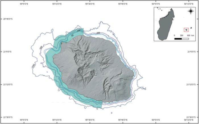
Reunion Island (21 07'S, 55 330 E) is a French oversea territory, located in the Mascarene archipelago, about 170 km
west from Mauritius Island and 700 km east of Madagascar in the southwestern Indian Ocean (Figure 1). As a young
volcanic island, Reunion Island has a narrow insular shelf with water depth steeply dropping off to 4,000 m at about
60 km from the nearest shore. Seabed substrate varies spatially around the island, from basaltic rocks to sandy bot-
tom. The windward east coast is frequently exposed to winds and heavy rainfall, while the leeward west coast is rela-
tively sheltered. The climate is tropical and humid, with two slightly marked seasons, and sea surface temperature
ranges from 24 C to 28 C throughout the year (Conand, Marsac, Tessier, & Conand, 2007).
Because survey effort mostly concentrated off the west coast (leeward), due to poor weather conditions and
logistical resources elsewhere, the study area was defined as the west coast of the island, from Saint Denis (north) to
Saint Joseph (south), up to three nautical miles offshore (Figure 1).
F I G U R E 1 Map of the study area around Reunion Island with isobaths from 50 m to 1,000 m (Source: Globice,
Natural Earth, IGN).4 ESTRADE AND DULAU
2.2 | Data collection
From 2010 to 2015, dedicated boat-based surveys were conducted all year-round within the study area using 6 m
motorboats and at an approximate speed of 6 knots on effort. Surveys were conducted in calm sea conditions
(Beaufort ≤3). During on-effort survey periods, three experienced observers (with one on each side of the boat and
one watching ahead) searched visually for dolphins with naked eyes and using continuous scanning method as
described by Mann (1999). Survey routes were tracked with a handheld geographical position system (GPS) Gar-
min 72H.
Whenever bottlenose dolphins were sighted, the survey route was curtailed, and the boat was slowed down to
carefully approach the animals to a point at which dorsal fins could be photographed. Distinction between Indo-
Pacific and common bottlenose dolphins was made based upon morphological features (i.e., body length, rostrum
size, shape of the dorsal fin, and presence/absence of spots; see Figure S1) and the species was confirmed a
posteriori by an experienced person (V.E.) based on photographs.
Several parameters were recorded upon sighting, such as the GPS position (latitude and longitude), date, time,
estimated group size (minimum, maximum and best estimate), group composition (number of calves and juveniles fol-
lowing the definition of age classes from Bearzi, Notarbartolo-Di-Sciara, & Politi, 1997), behavior at first encounter,
presence of other cetacean species, reaction to the research vessel, presence of other vessels around the animals,
and all other comments considered as relevant. Group size was visually estimated by at least two observers and aver-
aged. This field estimation was subsequently adjusted based on photo-identification data (Ballance, 1990). A group
was defined as an aggregation of dolphins within an area of a 100-m radius of each other, exhibiting similar behavior,
and if traveling, heading in the same direction (Shane, 1990; Wells, Scott, Stockin, & Irvine, 1987).
Photographs of bottlenose dolphin dorsal fins were obtained using Nikon D5000 or Canon 60S/90D digital cam-
era fitted with a 70–300 mm zoom lens. When possible, photographs of both left and right sides of each individual
dorsal fin were taken. Dolphins were photographed until the identification of each individual was completed, or the
focal group showed avoidance behavior, precluding further data collection.
2.3 | Individual identification and dorsal fin scoring
Each photograph was graded with a photo quality rating of poor, fair, good, and excellent. This criterion depends on
the focus, angle, clarity, contrast, and size of the dorsal fin within the picture (Slooten, Dawson, & Lad, 1992). Only
high-quality photographs (i.e., good or excellent), which related to focused pictures of the entire dorsal fin profile,
were retained for the analysis (Hammond, Mizrock, & Donovan, 1990; Read, Urian, Wilson, & Waples, 2003; Urian,
Hohn, & Hansen, 1999; Urian et al., 2015; Wilson, Hammond, & Thompson, 1999). Poor or fair quality photos were
removed from the analysis to avoid incorrect identifications (Friday, Smith, Stevick, & Allen, 2000).
High quality pictures were edited using PICASA 2.0 software to extract cropped images of each individual dorsal
fin. Dorsal fins were then sorted according to permanent marks. Other features such as dorsal fin shape, pigmenta-
tion, or temporary marks (tooth rakes, scars, skin alterations, bite wounds, etc.) were used as secondary identification
keys to confirm individual identification or to assist in identification of similarly marked individuals (Wilson
et al., 1999). The best image of each dolphin was compared to the photo-identification catalogue using DARWIN
1.9. Beta. Each individual dorsal fin that matched previously catalogued animal was considered a recapture, while
new individuals were added to the catalogue (Urian et al., 1999, 2015). To ensure homogeneity in the identification
process, one person (V.E.) double-checked all captures/recaptures made over the study period.
Individuals showing a dorsal fin with no mark on the trailing edge were classified as unmarked and not included
in the catalog. Each marked individual was assigned a marking level, according to the number, deepness, and extent
of its marks, ranging from D1 to D3, where D1 = slightly distinctive, D2 = distinctive, and D3 = very distinctive
(Dulau et al., 2017; Read et al., 2003; Urian et al., 1999; Urian et al., 2015; Wilson et al., 1999; Figure 2).ESTRADE AND DULAU 5
F I G U R E 2 Bottlenose dolphin dorsal fin photographs displaying different marking levels. (a) D1: Slightly
distinctive (i.e., with few notches along the trailing edge); (b) D2: distinctive (i.e., with moderated notches), and
(c) D3: very distinctive (with multiple and large notches, and/or deep nicks and cuts along the trailing edge or leading
edge, and/or disfigurements).
2.4 | Abundance estimates from mark-recapture models
Mark-recapture analysis was conducted by defining years (2010–2015) as sampling occasions and using the capture
history of well-marked individuals only (D2 and D3) in Mark 7.2 (White & Burnham, 1999). POPAN formulation of the
classic Jolly-Seber open population models were performed to assess abundance and demographic parameter esti-
mates, as gain (through immigration or birth) and loss of individuals (through permanent emigration or death) were
likely to occur over the 6-year survey (Crosbie & Manly, 1985; Jolly, 1965; Schwarz & Arnason, 1996; Seber, 1965).
2.4.1 | Model assumptions and data selection
Population closure was tested statistically using the CloseTest v3 program (Stanley & Burnham, 1999). Both Otis,
Burnham, White, and Anderson (1978) and Stanley and Burnham (1999) closure tests confirmed that the population
was not closed (χ2 = 72.0, df = 7, p < 1.10−4, and Z = −8.1, p < 1.10−4, respectively). A test for transience (Test 3.SR)
was also carried out in U-Care 2.3.2 (Choquet, Lebreton, Gimenez, Reboulet, & Pradel, 2009) and did not provide evi-
dence of transience (Z = 0.89, df = 4, p = .371).
The open Jolly-Seber capture-recapture model operates under several assumptions and their violation can lead
to biased population estimates (Amstrup, McDonald, & Manly, 2005; Read et al., 2003; Seber, 1982; Williams,
Nichols, & Conroy, 2002; Wilson et al., 1999). Each assumption was explored, and data was selected in order to meet
these assumptions, as follows:
1. Absence of mark loss and consistent mark recognition: (a) use of high-quality photographs to identify individuals;
(b) selection of well-marked individuals (marking levels D2 and D3 only) (Friday et al., 2000; Rosel et al., 2011;
Urian et al., 1999, 2015; Würsig & Jefferson, 1990); (c) year-round sampling, so marks were unlikely to change
significantly between two consecutive sampling occasions (Wilson et al., 1999); (d) use of temporary marks on
dorsal fin as secondary identification keys to confirm individual identification; and (e) validation of individual iden-
tification by an experienced observer (V.E.).
2. Equal probability of capture: (a) during sighting, individuals were photographed randomly, irrespective of their
levels of markings (Würsig & Jefferson, 1990); (b) calves were excluded from mark-recapture analysis because
their probability of capture was highly related to that of their mothers (Wells & Scott, 1990; Wells et al., 1987);
and (c) the pooled χ2 statistics (goodness-of-fit Test 2 in U-Care 2.3.2; Choquet et al., 2009) did not detect any
significant difference in capture probability in the population (χ2 = 9.2, df = 5, p > .10).
3. Equal survival probability: (a) the pooled χ2 statistics (goodness-of-fit Test 3 in U-Care 2.3.2; Choquet et al., 2009) did
not detect any significant difference in survival probability in the population (χ2 = 8.8, df = 8, p > .30).6 ESTRADE AND DULAU
4. Instantaneous sampling: sampling occasions were short in duration (1 year) compared to the dolphins' lifespan.
5. Absence of behavioral response to capture (Read et al., 2003; Wilson et al., 1999): (a) photo-identification being a
noninvasive mark-recapture method, inducing minimal stress to the animal, it is not expected to influence the
probability of subsequent recaptures; (b) Test 2.CT (Choquet et al., 2009; Pradel, 1993) in U-Care 2.3.2 did not
detect any trap-dependence behavior (Z = −1.35, df = 3, p = .177).
Despite selection of high-quality data, violation of some of these assumptions may still exist, as suggested by
the value of the post hoc variance factor ĉ (ĉ = 1.38 > 1) (Williams et al., 2002). This factor measures over-dispersion
in the data and is defined as the chi-square statistic from global test (TEST 2+ TEST 3) divided by its degrees of free-
dom. The estimated value of ĉ was thus used to adjust the models (Cooch & White, 2009).
2.4.2 | Population models
Maximum likelihood was used to estimate the following parameters: capture probability (p), apparent annual survival
rate (ɸ), probability of entry (Pent), and superpopulation size (ND) where: p(t) is the probability that an individual
available for capture in sampling occasion t would be captured in sampling occasion t + 1; ɸ(t) is the apparent sur-
vival probability from sampling occasion t to sampling occasion t + 1; Pent(t) is the probability of entry in the study
area between sampling occasion t to sampling occasion t + 1; and ND is the superpopulation size, defined by Crosbie
and Manly (1985) and Schwarz and Arnason (1996), corresponding to the total number of (well-marked) individuals
available for capture at any time within the survey area. The models provide an average superpopulation size for the
study period (6 years) as well as year estimates.
Different combinations of models were built by setting apparent annual survival, capture probability and proba-
bility of entry either constant (.) or time-varying (t) across sampling occasions (i.e., years). Models were fitted using a
sin link function for capture probability and apparent annual survival, a multinomial logit link function to constrain
entry probabilities to ≤1 and a log link function for the superpopulation size (Cooch & White, 2009).
2.4.3 | Model selection and parameters estimation
Given the extra-binomial dispersion of the data (ĉ > 1), the most suitable model was selected using the lowest Quasi
Akaike's Information Criterion corrected for small sample sizes (QAICc; Burnham & Anderson, 2002). Models differ-
ing by two units or less from the model with minimum QAICc (ΔQAICc) were also considered to provide a good
description of the data (Burnham & Anderson, 2002). Both real function and derived parameter values were provided
from the best-fitting model. The 95% confidence interval was calculated assuming a log-normal approximation, as
recommended by Burnham, Anderson, White, Brownie, and Pollock (1987).
2.4.4 | Proportion of (well-)marked individuals in the population
Abundance estimates obtained from the models only refer to the population of well-marked animals (marking level
D2 and D3). Therefore, the total population size Ntotal, including marked and unmarked individuals, was estimated by
considering the proportion θ of well-marked individuals in the population (Jolly, 1965; Seber, 1982; Wilson
et al., 1999) following:
Ntotal = ND =θESTRADE AND DULAU 7
where Ntotal is the total population size estimate; ND, the abundance estimate of well-marked individuals generated
from the best-fitting model, and θ, the estimated proportion of well-marked (D2 and D3) individuals in the population
(Burnham et al., 1987; Read et al., 2003; Wilson et al., 1999).
Theta (θ) was estimated using a sighting-based method (Fruet, Secchi, Di Tullio, & Kinas, 2011; Nicholson, Bejder,
Allen, Krützen, & Pollock, 2012), by computing for each sighting the number of well-marked (D2 and D3) individuals over
the estimated group size. To estimate θ with accuracy, only sightings for which the photographic coverage (Pc) was over
70% were used. The photographic coverage was defined as the percentage of marked individual (i.e., adults D1 to D3) on
the total number of adults estimated in the group, and calculated as follow (modified from Nicholson et al., 2012):
Xn
ðD1i + IiÞ
Pc = 100
i=1
ðTi −Ji− CiÞ
where D1i = total number of D1 individuals photographed in group i, Ii = total number of well-marked dolphins
(D2 and D3) photographed in group i, Ji = total number of juveniles estimated in group i, Ci = total number of calves
estimated in group i, Ti = total number of dolphins estimated in group i, and n = total number of sightings.
Furthermore, to reduce variance due to small sample sizes, groups with 70%).
The standard error for the total population size Ntotal was derived using the delta method as follows (modified
from Nicholson et al., 2012; Williams et al., 2002; Wilson et al., 1999):
vffiffiffiffiffiffiffiffiffiffiffiffiffiffiffiffiffiffiffiffiffiffiffiffiffiffiffiffiffiffiffiffiffiffiffiffiffiffiffiffiffiffiffiffiffiffiffiffiffiffiffiffiffiffi
0 2 1ffi
u
uu ^
uN
^total = t ^ 2B
SE ND 1− ^θC
SE N total @ + A
N^D 2
k^θ
As recommended by Burnham et al. (1987) and to better reflect the uncertainty in abundance estimates
(Buckland, Anderson, Burnham, & Laake, 1993), the 95% confidence interval for the total population size was com-
^total =Cand upper limit of N
puted assuming a lognormal approximation, with a lower limit of N ^total *C where:
0vffiffiffiffiffiffiffiffiffiffiffiffiffiffiffiffiffiffiffiffiffiffiffiffiffiffiffiffiffiffiffiffiffiffiffiffiffiffiffiffiffiffiffiffiffiffiffiffiffiffiffi
ffi
u 0 0 12 11
u ^
B u SE N C
ulnB
B1:96t
C = exp@ @1 + @
total
A C AC
N^total A
2.5 | Site fidelity and residency
Two metrics were used to assess individual site fidelity to the study area: (1) the total number of sightings of each
individual within the study area and (2) the residency time (number of days between the first capture and the last
recapture).8 ESTRADE AND DULAU
In order to have sufficient sample size and to avoid under-estimation, all marked individuals (D1 to D3 individ-
uals) except those first identified during the last year of the survey (2015, n = 9) were included in the site fidelity
analysis. To ensure the independence of the data, in cases where an individual was sighted several times on the same
day, only the sighting for which the number of identified individuals was the highest was used for that day.
To discriminate different residency patterns (i.e., short-term visitor, long-term visitor, and resident), a hierarchical
clustering analysis was performed based on the number of sightings and residency time of each identified individual,
using XLStat V 2.7 2017 (Addinsoft). Euclidean distance was used as a measure of dissimilarity; Ward's method as
the clustering algorithm (Ward, 1963) and automatic truncation was based on the entropy criterion. To test the effi-
ciency of the clustering and evaluate the suitability of the clusters, the cophonetic correlation coefficient (CCC) was
calculated (Sokal & Rohlf, 1962).
2.5.1 | Social structure
The half weight association index (HWI) was calculated via SOCPROG 2.7 (compiled version; Whitehead, 2009). The
HWI represents the proportion of times that each pair of individuals is seen in a group together and varies between
0 (individuals never seen together) and 1 (individuals always seen together) (Cairns & Schwager, 1987):
X
HWI =
X + 0:5ðY a + Y b Þ
where X is the number of groups where individuals A and B were seen together, Ya, the number of groups where
individual A was sighted without individual B and Yb, the number of groups where individual B was sighted without
individual A. This index is considered as the most suitable one for defining association in cases where it is not always
possible to identify all individuals in the group (Cairns & Schwager, 1987).
In order to account for the effects of structural factors that may affect associations, the generalized affiliation
indice (GAI) was used as a measure of the strength of association between pairs (also called true affiliation; White-
head & James, 2015). A multiple regression quadratic assignment procedure (MRQAP) was performed with 20,000
permutations, using the “double semi-partialing” technique of Dekker, Krackhardt, and Snijders (2007), to test the
effect of each potential structural factor, while controlling for the other, on the association indices (HWIs) matrix.
The contribution of each factor was assessed using the partial correlation coefficient, and those that did not signifi-
cantly explain the matrix of association indices were removed. GAIs were defined as the deviance residuals of the
generalized linear model, where the HWIs was the dependent variables and the structural factors, the predictor vari-
ables, and assuming a binomial model (Whitehead & James, 2015).
Because individuals that are frequently sighted or that use the study area at the same time tend to associate
more often with each other, two metrics were tested as structural factors: (1) the cumulative number of sightings for
each individuals' pair and (2) the temporal overlap by pair of individuals (defined as the ratio of the number of months
in which at least one individual from a pair was present to the number of months both were present in the study
area; adapted from Whitehead & James, 2015).
Individual gregariousness (i.e., the tendency for some individuals to be found in consistently smaller or larger
groups than others; Whitehead, Bejder, & Ottensmeyer, 2005) was tested using the Bejder, Fletcher, and
Bräger (1998) procedure, modified from Manly (1995) (with 10,000 permutations). The SD of the typical group sizes
observed (i.e., group sizes experienced by a given individual; Whitehead, 2009) was not significantly different from
random (SDobserved = 7.96, SDrandom = 8.00, p = .62), suggesting a lack of gregariousness in the population. Hence, this
metric was not taken into account for the calculation of GAIs.
To assess whether associations within residency patterns were significantly different than associations between
residency patterns, mean GAIs were compared via two-tailed Z-Mantel tests using 1,000 permutations. Furthermore,ESTRADE AND DULAU 9
Manly-Bejder permutation tests for preferred/avoided associations were performed across the whole population to
test the null hypothesis that individuals associate more often than expected by chance with other individuals (Bejder
et al., 1998; Manly, 1995; Whitehead, 1999, 2008, 2009; Whitehead et al., 2005). Then, permutations were run to
test for preferred/avoided associations within and between residency patterns. The null hypothesis was that individ-
uals associated with the same probability with all other individuals regardless of their residency pattern. To obtain a
consistent p-value, the number of permutations (groups within samples) was increased by 2,000 after each run until
the difference in p-values was 1.0), models were selected according to their QAIC. The model with
the lowest QAIC was selected as providing the best fit to the data (Whitehead, 2009).
3 | RESULTS
3.1 | Survey and photo-identification effort
A total of 1,187 daily surveys were conducted between 2010 and 2015, totaling 5,464 hr and 38,066 km of sampling
effort within the study area (Figure 3). A total of 126 bottlenose dolphin groups were sighted on 107 different days.
Photo-identification data was available for 89 of these sightings (see Table S1).
A total of 6,854 photographs were taken, from which 5,349 were of sufficient quality to allow identification for
subsequent photo-identification analysis. The photo-identification catalogue contained 187 marked individuals (D1:
33 slightly distinctive; D2: 83 distinctive and D3: 71 very distinctive).
Group size estimates ranged from 1 to 150 animals (mean = 24.5, SD = 24.9, median = 20.0), with the majority
of groups being smaller than 30 individuals (n = 94, 74.6%). The number of individuals photo-identified within a
group ranged from 1 to 49 (mean = 11.7, SD = 10.5). Of the 68 sightings for which photo-identification data were10 ESTRADE AND DULAU
F I G U R E 3 Survey effort (gray line) and sightings of bottlenose dolphins (white dot) per year in the study area,
from 2010 to 2015 (Scale: 1/1,000,000).
available and whose group size exceeded ten individuals, 27 (40%) showed a high photographic coverage (Pc) of
70% or above, and in six of them all individuals were photographed (Pc = 100%).
3.2 | Discovery curve
The cumulative number of well-marked dolphins (D2 and D3) increased sharply until mid-August 2011 (i.e., after
12 daily surveys), with an average of 5.1 new individuals discovered per month (Figure 4). Onwards, the discovery
curve increased much more gradually from mid-August 2011 to mid-August 2012 (i.e., after the 38th daily survey),
with an average of 2.3 individuals newly identified per month, and finally reached a plateau, suggesting that almost
all well-marked individuals of the population had been identified in the study area. The asymptote was reached dur-
ing the 50th daily survey.
3.3 | Abundance estimates
3.3.1 | Population models
Of the eight candidate models run using POPAN formulation, only one was selected as best supporting the data: {p
(.), ɸ(t), Pent(t)}. This model considers that the probability of capture of individuals remains constant, and that the
apparent survival rate and the probability of individuals entering the study area vary across years (Table 1). Other
models differed by more than two units in QAICc and were thus considered to show a lower fit to the data.
3.3.2 | Estimated parameters
The best fitting POPAN model provided (Table 2) (1) a high and constant capture probability (p = 0.74,SE = 0.03);
(2) an apparent annual survival rate (ɸ) ranging from 0.61 (SE = 0.09) in 2015 to 1.00 (SE = 0.03) in 2012; the average
annual survival rate was estimated to 0.83 (95% CI = 0.50–0.91); and (3) a relatively low probability of entry (Pent)ESTRADE AND DULAU 11
F I G U R E 4 Cumulative discovery curve for well-marked bottlenose dolphins identified off Reunion Island in the
study area over the period 2010–2015.
T A B L E 1 List of Jolly-Seber mark–recapture candidate models with POPAN parameterization ranked by
quasi-likelihood Akaike Information Criteria (QAICc). Only the top-four models are displayed. Models with ΔQAICc
≤2 were considered as best-fitting models.
Model QAICc ΔQAICc QAICc weight No. of parameters
{p(.), ɸ(t), Pent(t)} 564.1 0.0 0.94 11
{p(t), ɸ(.), Pent(t)} 569.9 5.8 0.05 13
{p(t), ɸ(t), Pent(t)} 573.3 9.1 0.01 17
{p(.), ɸ(.), Pent(t)} 577.0 12.8 0.002 7
Note. Survival probability: ɸ; recapture probability: p; probability of entering the study area: Pent. Each model incorporates
either constant (.) or time-varying (t) parameters.
ranging from 0.00 (SE = 0.00) in 2013 to 0.54 (SE = 0.07) in 2011, leading to an average probability of entry of 0.13
(95% CI = 0.08–0.40).
The annual estimate of the superpopulation size of well-marked individuals (ND) derived from the model ranged
from 58 (SE = 7.8, 95% CI = 44–75) in 2010 to 142 (SE = 5.2, 95% CI = 132–153) in 2012 (Table 2). The global super-
population size estimated for the 6 years study period was ND = 164 (SE = 4.6, 95% CI = 155–173).
3.3.3 | Proportion of well-marked individuals and total abundance
^ during the study period was 64.5% (SD = 13.7%,
The mean proportion of well-marked animals in the population (θ)
n = 27), giving a total population size estimate of Ntotal = 254 individuals (SE = 36.9, 95% CI = 191–337) over the
6 years (2010–2015).12 ESTRADE AND DULAU
T A B L E 2 Estimates of abundance parameters derived from the best Jolly-Seber candidate model with POPAN
parameterization {p(.), ɸ(t), Pent(t)}. Total population size (Ntotal) has been calculated from the superpopulation size
(ND) taking into account the proportion of well-marked animals in the population (θ).
Well-marked individuals Total population
Year N ND SE 95%CI θ Ntotal SE 95%CI
2010 43 58 7.8 44–75 0.60 96 79.8 23–397
2011 103 136 8.2 121–153 0.88 156 59.6 75–321
2012 109 142 5.2 132–153 0.66 216 52.1 135–344
2013 84 121 6.7 108–135 0.68 179 47.8 107–299
2014 71 101 7.8 87–117 0.59 170 64.7 83–350
2015 48 66 8.2 52–84 0.58 114 50.6 50–262
Note. SE: standard error; 95%CI: 95% log-normal confidence intervals, N: number of different marked individuals encoun-
tered per year.
3.4 | Site fidelity and residency
Of the 187 individuals from the catalog (marking level D1 – D3), 175 were first identified prior to 2015 and included
in the site fidelity analysis.
3.4.1 | Individual recaptures
During the study period, individuals were sighted 1–26 times (mean = 5.7, SD = 4.8). Twenty-six individuals (14.9%)
were transients (i.e., individuals sighted only once), 61 (34.9%) were sighted on less than five occasions, whereas
65 individuals (37.1%) were resighted from five to ten times. Twenty-three individuals (13.1%) were sighted >10
times.
3.4.2 | Residency time
For the 149 individuals (85.1%) sighted more than once during the study period, the mean residency time was 1,043
± 522 days (i.e., ~3 years), ranging from 21 to 2,024 days. The majority of individuals (n = 126, 84.6%) used the study
area between 300 (~1 year) and 1,800 days (~5 years). Nine individuals resided less than 300 days (6.0%), whereas
14 animals were observed over more than 1,800 days (9.4%).
The hierarchical clustering analysis provided a CCC of 0.635, suggesting a reliable discrimination of individuals
into three clusters, indicative of three main patterns of site fidelity (Figure 5). The first cluster consisted of 60 indi-
viduals rarely sighted (number of sightings = 2.2 ± 1.3) and displaying low residency time (186 ± 197 days). This
cluster represented “short-term visitors” (hereafter STV) and included transients (n = 26). The second cluster
included 58 individuals frequently sighted (mean number of sightings = 10.7 ± 4.9) and displaying high residency
(mean residency time = 1,529 ± 319 days) indicating that they consistently occurred within the survey area, across
multiple years (but not necessarily consecutive). These individuals were classified as “residents.” The third cluster
was composed of 57 individuals not frequently observed in the study area (number of sightings = 4.4 ± 1.7) but
over long period (medium residency time of 975 ± 215 days). This cluster reflected “long-term visitors” (hereaf-
ter LTV).ESTRADE AND DULAU 13
3.4.3 | Social structure
MRQAP correlation tests showed that the temporal overlap was a relevant structural factor for explaining the matrix
of association indices (partial correlation coefficient = 0.899, p < .0001). In contrast, the cumulative number of
sightings did not show a significant contribution (partial correlation coefficient = 0.002, p > .99) and was therefore
removed for the calculation of GAIs.
Associations of individuals within and between residency patterns were significantly different (two-tailed Mantel
test, t = 6.48, r = 0.048, p < .0001). Maximum mean GAI was displayed by resident individuals (mean GAI = −0.031,
SD = 0.81) while minimum mean GAI was observed within STV individuals (mean GAI = −0.35, SD = 0.39; Table 3).
Permutation tests performed on the overall population indicated that individuals associated randomly. Indeed,
neither the mean GAI nor the SD of GAI of the observed population were significantly different from random (mean
GAIobserved = −0.212, GAIrandom = −0.215, p = .94 and SDobserved = 0.621, SDrandom = 0.626; p = .96, respectively;
Table 3).
Within each residency pattern, except for residents, neither the mean GAI nor the SD of GAI of the observed
data were significantly different from random, indicating a probable absence of preferred or avoided associations.
For resident individuals, the mean GAI of the observed data was significantly higher than that of randomly permuted
data (mean GAIobserved = −0.031, GAIrandom = −0.067, p = .0001; Table 3), which was not considered biologically
meaningful (Whitehead, 2009).
The modularity of the population (from gregariousness) of 0.020 indicated that the population was not divided
into communities. The social network diagram did not display any cluster featuring the three residency patterns. In
F I G U R E 5 The agglomerative hierarchical clustering analysis (AHC) showing how individual bottlenose dolphins
clustered according to the two metrics describing site fidelity: number of sightings and residency time. The
dissimilarity threshold displays three clusters: the cluster 1 (i.e., residents, n = 58) in blue, the cluster 2 (i.e., long-term
visitors, n = 57) in red and the cluster 3 (i.e., short-term visitors, n = 60) in green.14 ESTRADE AND DULAU
contrast, it formed an intricate network, where individuals associated irrespective of their residency pattern (see
Figure S2). In particular, STV and LTV mixed with resident individuals.
3.4.4 | Lagged identification rate
LIR analysis revealed that the model that best described the data (with the lowest QAIC) included emigration and
reimmigration (Table 4). This model estimated that individuals were present within the study area for an average
period of 832 days. The average subsequent time spent outside the study area before returning was estimated at
approximately 276 days.
The LIR curve started to decay after about 25 days suggesting that some individuals leave the study area
through emigration. After 900 days, the fitted model began to level off above zero, indicating that a number of indi-
viduals subsequently return to the study area and/or that some animals frequently use the study area as residents.
The shape of the LIR curve tends to be indicative of a mixture of individuals with different levels of residency
(i.e., residents, LTV and STV) (Figure 6).
4 | DISCUSSION
By assessing demographic parameters, residency patterns and social structure over a 6-year period off Reunion
Island, this study provided baseline information on the ecology and behavior of island-associated bottlenose dol-
phins. This population was shown to be demographically open and had an estimated abundance of 254 individuals
(95% CI = 191–337, 2010–2015). Although the species was present year-round in relatively large groups (mean
group size = 24.5 animals, SD = 24.9), pattern of residency varied among individuals: a third of the individuals
exhibited high site fidelity, and were considered as residents (33.1%), while others were short or long-term visitors,
in similar proportion (34.3% and 32.6%, respectively). Individuals showing different residency patterns associated
randomly; they mingled together into mixed groups, forming a single community.
4.1 | Limits of the open Jolly Seber model
Even if Jolly Seber open capture-recapture models address biases related to the assumption of population closure,
their use involves numerous assumptions that have to be explored and validated (Begon, 1983; Read et al., 2003;
T A B L E 3 Results from permutations tests for preferred/avoided associations across the three residency patterns
(i.e., resident, RES; long-term visitor, LTV; and short-term visitor, STV).
mean GAII SD
Residency pattern n observed data random data p observed data random data p
RES 58 −0.0306 −0.0669 0.0001* 0.81244 0.81335 0.542
LTV 57 −0.12427 −0.12297 0.2983 0.59798 0.61325 0.9981
STV 59 −0.34846 −0.34775 0.3799 0.38781 0.38683 0.4932
RES-LTV — −0.09982 −0.10255 0.8814 0.71481 0.72058 0.9448
RES-STV — −0.30996 −0.30981 0.4743 0.61262 0.61096 0.2498
LTV-STV — −0.28387 −0.28279 0.1785 0.46265 0.46184 0.4047
Note. Significant p-values are indicated by an asterisk.ESTRADE AND DULAU 15
T A B L E 4 Models fitted to observed lagged identification rate (LIR) data of common bottlenose dolphin
population in the study area during the period 2010–2015. Explanation of each model refers to Whitehead (2001).
The model that best fitted the data according to QAIC (i.e., Akaike's information criterion corrected for
overdispersion) is shown in bold. For the best fitting model, a1 = N, number of individuals present within the study
area at any one time, a2 = mean residency time in, and a3 = mean residency time out the study area.
Model
Model Explanation QAIC ΔQAIC evaluation
(1/a1)*((1/a3) + (1/a2)*exp(−(1/a3 + 1/a2)*td))/ Emigration 22,670.0180 - Best
(1/a3 + 1/a2) +reimmigration
(1/a1)*exp(−td/a2) Emigration+mortality 22,672.3236 2.3056 No support
a2*exp(−a1*td) Emigration+mortality 22,672.3237 2.3057 No support
a3*exp(−a1*td) + a4*exp(−a2*td) Emigration 22,676.3236 6.3056 No support
+reimmigration
+mortality
(exp(−a4*td)/a1)*((1/a3) + (1/a2)*exp Emigration 22,675.9737 5.9557 No support
(−(1/a3 + 1/a2)*td))/(1/a3 + 1/a2) +reimmigration
+mortality
1/a1 Closed 22,680.4038 10.3858 No support
a1 Closed 22,680.4038 10.3858 No support
a2 + a3*exp(−a1*td) Emigration 22,683.6727 13.6547 No support
+reimmigration
F I G U R E 6 Lagged identification
rate of marked common bottlenose
dolphins in the study area during the
period 2010–2015. The curve was
generated using the movement
analysis section of the compiled
version of SOCPROG 2.7
(Whitehead, 2009), with maximum
time lag fixed to 2,043 days.
Bootstrap error bars, calculated from
100 replications/iterations are shown
on the graph.
Seber, 1982; Wilson et al., 1999). Although effort was made to minimize biases, violations of some assumptions may
exist, as suggested by the post-hoc variance factor value (ĉ = 1.38 > 1; Williams et al., 2002). Homogeneity in capture
probability is typically one of the key assumptions underlying POPAN models (Gilbert, 1973; Seber, 1982). Despite
different patterns of residency found among individuals, the pooled χ2 statistics for Test 2 showed a probable lack of
heterogeneity of probabilities of capture in the population. Test 3.SR did not detect transience, although part of the
population (n = 26, 14.9%) was described as transient. This can be due to the low power of this test in detecting tran-
sients with reduced sample sizes (Pradel, Hines, Lebreton, & Nichols, 1997). The presence of transients might explain16 ESTRADE AND DULAU
the observed ĉ value and caused an underestimation of the apparent survival rate (Pledger, Pollock, & Norris, 2003;
Pollock & Alpizar-Jara, 2005). However, the lack of fit displayed by the ĉ value was limited (≤3) and might have
resulted from extrabinomial noise rather than by inappropriate model used.
4.2 | Demographic parameters
4.2.1 | Group size
The average group size described in Reunion Island (mean = 24.5, median = 20.0, 1–150) was consistent with off-
shore populations (Cañadas & Hammond, 2006; Hansen, 1990) or remote oceanic island-associated populations (S~ao
Tomé Island: Pereira et al., 2013; Azores Archipelago, Portugal: Silva et al., 2008); an exception being Hawaii, where
bottlenose dolphins tend to form smaller groups (i.e., mean = 6.3, SD = 4.5, median = 6: Baird, Gorgone, Ligon, &
Hooker, 2001). Group sizes estimated for bottlenose dolphins inhabiting enclosed environments are generally smaller
(i.e., generally less than 15 individuals per group in Santa Monica Bay, CA: Bearzi, 2005; Shannon Estuary, Ireland:
Berrow, O'Brien, Groth, Foley, & Voigt, 2012; Bay of Islands, New Zealand: Constantine, 2002; Moray Firth, Scot-
land: Eisfeld, 2003; Mississipi Sound, MS: Hubard, Maze-Foley, Mullin, & Schroeder, 2004; Ría de Arousa, Spain:
Methion & Díaz López, 2018; Charleston, NC: Speakman et al., 2006).
Resource availability and predation risk are known to affect group size in small delphinids, including in Tursiops
spp. (Gygax, 2002; Heithaus & Dill, 2002; Shane, Wells, & Würsig, 1986; Wells et al., 1987). The formation of larger
groups in oceanic waters could be linked to an increased vulnerability to predators and an adaptation to maximize
foraging efficiency where resources are scarce (Dinis et al., 2016; Norris & Dohl, 1980; Shane et al., 1986; Wells,
Irvine, & Scott, 1980). Little is known about the diet of bottlenose dolphins off Reunion Island. Predation risk on
bottlenose dolphins might occur in Reunion waters, as bull and tiger sharks are known to be present around the
island. However, in contrast to the coastal Indo-Pacific bottlenose dolphins, for which 19.8% of individuals displayed
shark-inflicted injuries (Heithaus et al., 2017), very few scars were observed on the common bottlenose dolphins
(V.D., V.E., personal observation). To date, only one individual has been photographed in 2017 with a fresh circular
bite wound behind the dorsal fin indicative of a shark attack injury (V.D., personal observation).
4.2.2 | Abundance estimate
The bottlenose dolphin population that used the study area during 2010–2015 was estimated to comprise 254 indi-
viduals (95% CI = 191–337). This abundance estimate was low compared to other populations using island-
associated habitats which tend to be characterized by large population size, with several hundreds to thousands of
individuals being generally reported (Balearic islands, Spain, Forcada et al., 2004; Hawaiian islands, Mobley, Spitz,
Forney, Grotefendt, & Forestell, 2000; Azores archipelago, Portugal, Silva et al., 2008). This difference could be due
to the carrying capacity of the habitat, whereby low productivity, remoteness, and small island size could limit the
size of the population that Reunion Island can sustain.
4.2.3 | Apparent survival rate
The annual apparent survival rate of adult bottlenose dolphins in Reunion Island was 0.83 (SE = 0.06) on average.
This apparent survival rate was relatively high, as expected for long-lived and slowly reproductive mammals (Connor
et al., 2000; Stolen & Barlow, 2003; Wells & Scott, 1999). The estimate was lower than values reported for other
populations of bottlenose dolphins (coastal or estuarine resident populations: Doubtful Sound, New Zealand: 0.94;ESTRADE AND DULAU 17
Currey et al., 2008; Patos Lagoon Estuary, Brazil: 0.89; Fruet et al., 2015; Sado Estuary, Portugal: 0.96, SE = 0.012;
Gaspar, 2003; Charleston, NC: 0.95, SE = 0.035; Speakman et al., 2010; Sarasota Bay, FL: 0.96, SD = 0.008; Wells &
Scott, 1990; and open ocean populations: Little Bahama Bank, USA: 0.94 – Fearnbach, Durban, Parsons, &
Claridge, 2012; Azores, Portugal: 0.97, SE = 0.03; Silva, Magalhaes, Prieto, Santos, & Hammond, 2009). Lower appar-
ent survival rate in more oceanic habitats might reflect higher predation pressure but also some level of permanent
emigration, which cannot be discriminated from mortality (Pledger et al., 2003). This would be consistent with the
residency patterns observed in this study, where the population seems to include transient individuals
(n = 26, 14.9%).
4.3 | Residency pattern
The low proportion of animals seen only once, together with the flat discovery curve, suggested that the majority of
the population in Reunion Island showed a high level of site fidelity. The LIR analysis estimated that individuals were
within the study area for a period of 832 days and remained outside of the survey area for 276 days on average.
During this period, individuals might remain in Reunion Island and use other areas around the island, being thus
unavailable for recapture. In fact, individuals identified outside of the study area, on the east coast of the island (not
considered in the present study), were all sighted at least once in the study area during the survey period (with the
exception of one individual), indicating individual movements around the island. Alternatively, some individuals might
use offshore habitats, or temporary migrate to other neighbouring islands such as Mauritius, Madagascar, or Rodri-
gues (170 km, 700 km, and 840 km away, respectively).
The high proportion of individuals showing high residency in the study area was relatively unexpected.
Populations using open-water habitats are usually characterized by a low recapture rate and low site fidelity (Defran,
Weller, Kelly, & Espinosa, 1999), although variations in residency patterns have been observed among oceanic
islands. Off Madeira, a remote island located 500 km off the northwest coast of Africa, a small proportion (21%, com-
pared to 75% in Reunion Island) of the bottlenose dolphin population was resighted in more than one year and only
3.2% showed long-term site-fidelity (i.e., seen in four or more years) (Dinis et al., 2016). Similarly, high proportions of
individuals sighted only once (between 35.2% and 65.7%, compared to 14.9% in this study), and hence showing low
site fidelity, have been reported in other remote oceanic islands (Northwestern Sardinian island: Díaz López,
Alberto, & Francesca, 2013; S~
ao Tomé Island, Portugal: Pereira et al., 2013; Azores islands, Portugal: Silva
et al., 2008). In contrast, in the Hawaiian archipelago, bottlenose dolphins display high site fidelity and low inter-
island movements, spending most of their time on the insular slope (18 ESTRADE AND DULAU and Porto Santo Island, 50 km apart (Dinis et al., 2016). Within Azores archipelago, Silva et al. (2008) showed that transient individuals could travel almost 300 km between islands. Moreover, studies from radio-tracking, genetics or photo-identification worldwide have suggested that individual bottlenose dolphins from offshore or island- associated populations may move great distances of several hundred kilometers (Klatsky, Wells, & Sweeney, 2007; Querouil et al., 2007; Tanaka, 1987; Tezanos-Pinto et al., 2009; Wells et al., 1999). Given such known dispersal abili- ties and the relative proximity of Mauritius and Rodrigues, long-range movements within the Mascarene islands (Reunion Island, Mauritius and Rodrigues) are likely to occur. Large-scale aerial surveys reporting the presence of bottlenose dolphins in oceanic waters of the southwest Indian Ocean, and more specifically at mid-distance between Reunion Island and Mauritius (Laran et al., 2017) tend to support this hypothesis. Nevertheless, to date, no studies have been conducted on possible interisland movements of bottlenose dolphins and the level of dispersal and con- nectivity among islands in this region is unknown. Future genetic and photo-identification studies should aim at assessing the connectivity and the level of dispersal within the Mascarene islands and among populations of the southwestern Indian Ocean. 4.4 | Social structure Despite significant differences of associations detected among individuals within and between residency patterns (via the Mantel test), tests for preferred/avoided associations failed to detect nonrandom associations at both the overall population and residency patterns levels. Moreover, the Newman's modularity value (
ESTRADE AND DULAU                                                                                                       19

individuals showing low levels of site fidelity are less likely to associate with others. Hence, in a population where
individuals displayed different residency patterns, preferred associations were expected to occur within residency
patterns, potentially leading to the segregation of the population into communities based on residency pattern. How-
ever, this was not observed in this study. In Reunion Island, although individuals were shown to display high site
fidelity and diverse residency patterns, the population did not show any clear social structuring based on true affilia-
tions. The temporal overlap was shown to be a structural factor affecting association pattern, which suggested that
although individuals happen to occur in the study area at the same time, they associated by chance rather than dis-
playing any preferred or avoided association.

4.5     |   Conservation perspectives

This study represents the first comprehensive assessment of the bottlenose dolphin population dynamics and resi-
dency around Reunion Island. The demographic parameters (abundance, immigration, survival rates) estimated in this
study constitute fundamental insights to better define the conservation status of the species, which to date has been
locally considered as Data Deficient (UICN France et al., 2013). The local population was estimated at 254 individuals
(95% CI: 191–337), which is close to the threshold used by the IUCN guidelines to define endangered populations
(i.e., 250 individuals). Our estimates also suggest low levels of mortality and/or permanent emigration (as displayed
by the apparent survival rate) and high levels of site fidelity and residency for some individuals, although some level
of temporary emigration (visitors) and presence of transients were also observed. The presence of an important pro-
portion of resident individuals, which was relatively unexpected for a remote oceanic island, suggests that part of
the population might be particularly vulnerable to anthropogenic impacts if subjected to repeated interactions with
human activities.
      Dolphin-watching activities has been demonstrated to induce habitat and short-term behavioral changes on
odontocetes that could lead to a modification of the energy budgets, by increasing physical demands and/or reduc-
ing energy intake (Bejder et al., 2006a; Christiansen, Rasmussen, & Lusseau, 2013; Lusseau, Bain, Williams, &
Smith, 2009; Williams, Lusseau, & Hammond, 2006). These negative short-term impacts could lead to long-term indi-
vidual and even population-level effects, by affecting fitness and reproductive success (Bejder et al., 2006a,b; Inter-
national Whaling Commission, 2006; Lusseau, 2003). Therefore, in the light of growing whale-watching and
swimming with dolphins' activities, the development of responsible practices through public awareness, sustainable
management and law enforcement is strongly recommended. Results provided in this study will serve as baseline
information to support and substantiate these actions.

ACKNOWLEDGMENTS
We are grateful to all Globice's volunteers for their involvement in the fieldwork. We thank the Conseil Régional de
la Réunion, the European Union, and DEAL Réunion for having funded part of this study. We appreciate the recom-
mendation from Dr. Guido Parra and the contribution of three anonymous reviewers for their constructive com-
ments on the manuscript.

ORCID
Vanessa Estrade      https://orcid.org/0000-0003-2650-8518
Violaine Dulau      https://orcid.org/0000-0002-2228-3959

RE FE R ENC E S
Amstrup, S. C., McDonald, T. L., & Manly, B. F. J. (2005). Handbook of capture-recapture analysis. Princeton, NJ: Princeton
   University Press.
20 ESTRADE AND DULAU
Baird, R. W., Gorgone, A. M., Ligon, A. D., & Hooker, S. K. (2001). Mark-recapture abundance estimate of bottlenose dolphins
(Tursiops truncatus) around Maui and Lana‘i, Hawai‘i, during the winter of 2000/2001. (Unpublished National Marine Fish-
eries Service Report). Available from Southwest Fisheries Center, National Marine Fisheries Service, 8604 La Jolla
Shores Drive, La Jolla, CA 92037-1508.
Baird, R. W., Gorgone, A. M., McSweeney, D. J., Ligon, A. D., Deakos, M. H., Webster, D. L., … Mahaffy, S. D. (2009). Popula-
tion structure of island-associated dolphins: Evidence from photo identification of common bottlenose dolphins
(Tursiops truncatus) in the main Hawaiian Islands. Marine Mammal Science, 25, 251–274.
Baker, I., O'Brien, J., McHugh, K., Ingram, S. N., & Berrow, S. (2017). Bottlenose dolphin (Tursiops truncatus) social structure
in the Shannon Estuary, Ireland, is distinguished by age- and area-related associations. Marine Mammal Science, 34,
458–487.
Ballance, L. (1990). Residence patterns, group organization, and surfacing associations of bottlenose dolphins in Kino Bay,
Gulf of California. In S. Leatherwood & R. Reeves (Eds.), The bottlenose dolphin (pp. 267–283). New York, NY: Academic
Press.
Balmer, B. C., Wells, R. S., Nowacek, S. M., Nowacek, D. P., Schwacke, L. H., McLellan, W. A., … Pabst, D. A. (2008). Seasonal
abundance and distribution patterns of common bottlenose dolphins (Tursiops truncatus) near St. Joseph Bay, Florida,
USA. Journal of Cetacean Research and Management, 10, 157–167.
Bearzi, M. (2005). Aspects of the ecology and behavior of bottlenose dolphins (Tursiops truncatus) in Santa Monica Bay, Cali-
fornia. Journal of Cetacean Research and Management, 7, 75–83.
Bearzi, G., Notarbartolo-Di-Sciara, G., & Politi, E. (1997). Social ecology of bottlenose dolphins in the Kvarneri (Northern
Adriatic Sea). Marine Mammal Science, 13, 650–668.
Begon, M. (1983). Abuses of mathematical techniques in ecology: Application of Jolly's capture-recapture method. Oikos,
40, 155–158.
Bejder, L., Fletcher, D., & Bräger, S. (1998). A method for testing association patterns of social animals. Animal Behaviour, 56,
719–725.
Bejder, L., Samuels, A., Whitehead, H., & Gales, N. (2006a). Interpreting short-term behavioral responses to disturbance
within a longitudinal perspective. Animal Behaviour, 72, 1149–1158.
Bejder, L., Samuels, A., Whitehead, H., Gales, N., Mann, J., Connor, R., … Krützen, M. (2006b). Decline in relative abundance
of bottlenose dolphins exposed to long-term disturbance. Conservation Biology, 20, 1791–1798.
Berrow, S., O'Brien, J., Groth, L., Foley, A., & Voigt, K. (2012). Abundance estimate of bottlenose dolphins (Tursiops truncatus)
in the lower River Shannon candidate Special Area of Conservation, Ireland. Aquatic Mammals, 38, 136–144.
Best, P. B. (2007). Whales and dolphins of the southern African subregion. Cape Town, South Africa: Cambridge University
Press.
Borgatti, S. (2002). NetDraw: Network visualization [Computer software]. Harvard, MA: Analytic Technologies.
Buckland, S. T., Anderson, D. R., Burnham, K. P., & Laake, J. L. (1993). Distance sampling: Estimating abundance of biological
populations. London, UK: Chapman and Hall.
Burnham, K. P., & Anderson, D. R. (2002). Model selection and multimodel inference: A practical information theoretic approach.
New York, NY: Springer-Verlag.
Burnham, K. P., Anderson, D. R., White, G. C., Brownie, C., & Pollock, K. H. (1987). Design and analysis methods for fish sur-
vival experiments based on release-recapture. Bethesda, MD: American Fisheries Society.
Cairns, S. J., & Schwager, S. J. (1987). A comparison of association indexes. Animal Behaviour, 35, 1454–1469.
Cañadas, A., & Hammond, P. (2006). Model-based abundance estimates for bottlenose dolphins off southern Spain: implica-
tions for conservation and management. Journal of Cetacean Research and Management, 8, 13–27.
Cantor, M., Wedekin, L. L., Guimar~aes, P. R., Daura-Jorge, F. G., Rossi-Santos, M. R., & Simões-Lopes, P. C. (2012). Dis-
entangling social networks from spatiotemporal dynamics: The temporal structure of a dolphin society. Animal Behaviour,
84, 641–651.
Choquet, R., Lebreton, J. D., Gimenez, O., Reboulet, A. M., & Pradel, R. (2009). U-CARE: Utilities for performing goodness of
fit tests and manipulating CApture-REcapture data. Ecography, 32, 1071–1074.
Christiansen, F., Rasmussen, M. H., & Lusseau, D. (2013). Inferring activity budgets in wild animals to estimate the conse-
quences of disturbances. Behavioral Ecology, 24, 1415–1425.
Cockcroft, V. G., Ross, G. J. B., & Peddemors, V. M. (1990). Bottlenose dolphin, Tursiops truncatus, distribution in Natal's
coastal waters. South African Journal of Marine Science, 9, 1–11.
Conand, F., Marsac, F., Tessier, E., & Conand, C. (2007). A Ten-year period of daily sea surface temperature at a coastal sta-
tion in Reunion Island, Indian Ocean (July 1993–April 2004): Patterns of variability and biological responses. Western
Indian Ocean Journal of Marine Science, 6, 1–16.
Connor, R. C., Wells, R., Mann, J., & Read, A. J. (2000). The bottlenose dolphin: Social relationships in a fission-fusion society.
In J. Mann, R. C. Connor, P. L. Tyack, & H. Whitehead (Eds.), Cetacean societies: Field studies of dolphins and whales
(pp. 91–125). Chicago, IL: University of Chicago Press.You can also read