Affinity Fusion Graph-based Framework for Natural Image Segmentation
←
→
Page content transcription
If your browser does not render page correctly, please read the page content below
IEEE TRANSACTIONS ON MULTIMEDIA, VOL. 00, NO. 0, * 2021                                                                                                    1

                                         Affinity Fusion Graph-based Framework for Natural
                                                         Image Segmentation
                                                                          Yang Zhang, Moyun Liu, Jingwu He, Fei Pan, and Yanwen Guo

                                            Abstract—This paper proposes an affinity fusion graph frame-
                                         work to effectively connect different graphs with highly discrim-
                                         inating power and nonlinearity for natural image segmentation.
                                         The proposed framework combines adjacency-graphs and kernel
arXiv:2006.13542v3 [cs.CV] 15 Jan 2021

                                         spectral clustering based graphs (KSC-graphs) according to a
                                         new definition named affinity nodes of multi-scale superpixels.
                                         These affinity nodes are selected based on a better affiliation                      (a) Input image       (b) Superpixels (s1)     (c) Superpixels (s2)
                                         of superpixels, namely subspace-preserving representation which
                                         is generated by sparse subspace clustering based on subspace
                                         pursuit. Then a KSC-graph is built via a novel kernel spectral
                                         clustering to explore the nonlinear relationships among these
                                         affinity nodes. Moreover, an adjacency-graph at each scale is
                                         constructed, which is further used to update the proposed KSC-
                                         graph at affinity nodes. The fusion graph is built across different                (d) Superpixels (s3)    (e) Adjacency-graph          (f) `0 -graph
                                         scales, and it is partitioned to obtain final segmentation result. Ex-
                                         perimental results on the Berkeley segmentation dataset and Mi-
                                         crosoft Research Cambridge dataset show the superiority of our
                                         framework in comparison with the state-of-the-art methods. The
                                         code is available at https://github.com/Yangzhangcst/AF-graph.
                                           Index Terms—Natural image segmentation, affinity fusion
                                         graph, kernel spectral clustering, sparse subspace clustering,                        (g) GL-graph           (h) AASP-graph             (i) AF-graph
                                         subspace pursuit                                                               Fig. 1. Comparison results by different graph-based segmentation methods.
                                                                                                                        Although superpixel features vary greatly at different scales (s1∼s3), our AF-
                                                                                                                        graph can achieve the best performance.
                                                                   I. I NTRODUCTION

                                         I   MAGE segmentation is a fundamental yet challenging
                                             task in computer vision, playing an important role in
                                         many practical applications [1]. In the past few years, many
                                                                                                                        embody both spatial and feature information [4], forming
                                                                                                                        an intermediate image representation for better segmentation.
                                         image segmentation methods have been developed, which                          Some representative methods rely on building an affinity graph
                                         are roughly classified into supervised, semi-supervised, and                   according to the multi-scale superpixels [5]–[8]. Especially
                                         unsupervised methods. In some scenarios, supervised methods                    for affinity graph-based methods, segmentation performance
                                         cannot provide a reliable solution when it is difficult to obtain              significantly depends on the constructed graph with particular
                                         a large number of precisely annotated data. Because no prior                   emphasis on the graph topology and pairwise affinities be-
                                         knowledge is available, unsupervised image segmentation is a                   tween nodes.
                                         challenging and intrinsically ill-posed problem. Unsupervised
                                                                                                                           As shown in Fig. 1, adjacency-graph [5] usually fails to
                                         methods still receive much attention, because images are
                                                                                                                        capture global grouping cues, leading to wrong segmentation
                                         segmented without user intervention.
                                                                                                                        results when the objects take up large part of the image. `0 -
                                            In the literature, many unsupervised segmentation methods
                                                                                                                        graph [6] approximates each superpixel with a linear combi-
                                         have been intensively studied [2], [3]. Among them, unsu-
                                                                                                                        nation of other superpixels, which can capture global grouping
                                         pervised graph-based methods usually represent the image
                                                                                                                        cues in a sparse way. But it tends not to emphasize the
                                         content, which have become popular. Because the graphs can
                                                                                                                        adjacency, easily incurring isolated regions in segmentation.
                                            Manuscript received ** **, 2020; revised ** **, 2021. This work was         Both GL-graph [7] and AASP-graph [8] combine adjacency-
                                         supported in part by the National Natural Science Foundation of China (Grant   graph with `0 -graph by local and global nodes of superpixels,
                                         62032011, 61772257 and 61672279), the Fundamental Research Funds for
                                         the Central Universities 020214380058, and the program B for Outstanding       achieving a better segmentation than a single graph. These
                                         PhD candidate of Nanjing University 202001B054. (Corresponding author:         nodes are classified adaptively according to superpixel areas in
                                         Yanwen Guo.)                                                                   GL-graph and superpixel affinities in AASP-graph. However,
                                            Y. Zhang, J. He, F. Pan, and Y. Guo are with the National Key
                                         Laboratory for Novel Software Technology, Nanjing University, Nanjing          there still exist three difficulties to be solved: i) it is not reliable
                                         210023, China (e-mail: yzhangcst@smail.nju.edu.cn; hejw005@gmail.com;          to determine a principle for graph combination, which usually
                                         felix.panf@outlook.com; ywguo@nju.edu.cn).                                     relies on empiricism; ii) local and global nodes are not simply
                                            M. Liu is with the School of Mechanical Science and Engineering,
                                         Huazhong University of Science and Technology, Wuhan 430074, China (e-         and easily defined because superpixel features change greatly
                                         mail: lmomoy8@gmail.com).                                                      at different scales, especially for superpixel areas; iii) linear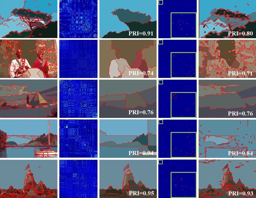
IEEE TRANSACTIONS ON MULTIMEDIA, VOL. 00, NO. 0, * 2021                                                                             2

graphs, such as `0 -graph, fail to exploit nonlinear structure      have been developed in recent years. These methods can be
information of multi-scale superpixels.                             roughly classified into two categories depending on whether
   To solve these problems, we first need to explore the rela-      the process of graph construction is unsupervised or not.
tionship between different graphs in principle. For graph-based        Unsupervised methods represent the image content with
segmentation, it is common to approximate the features of           static graphs or adaptive graphs. In static graphs, hard decision
each superpixel using a linear combination of its neighboring       is used to select connected nodes, and pairwise similar-
superpixels. Such an approximation is regarded as subspace-         ity is computed without considering other superpixels. An
preserving representation between neighboring superpixels [9],      adjacency-graph [5] is built upon each superpixel which is
which is perceived to be the theoretical guidance of graph          connected to all its neighborhoods. The pairwise similarity
combination. Because of the sparsity in subspace-preserving         is computed by Gaussian kernel function which is influ-
representation, its variation is not obvious. Given a subspace-     enced easily by the standard deviation [12], [13]. In adaptive
preserving representation of superpixels in each scale, we build    graphs, pairwise similarity is computed on all data points.
an affinity matrix between every pair superpixels (nodes) and       Wang et al. [6] proposed a `0 -graph by building an affinity
apply spectral clustering [10] to select affinity nodes. However,   graph using `0 sparse representation. The GL-graph [7] and
due to the linearity of the representation, segmentation with       AASP-graph [8] are fused by adjacency-graph [5] and `0 -
linear graphs easily result in isolated regions, such as `0 -       graph [6], which can achieve a better result than a single
graph. To enrich the property of fusion graph while improving       graph. Yin et al. [14] utilized a bi-level segmentation operator
segmentation performance, it is necessary to capture nonlinear      to achieve multilevel image segmentation, which determines
relationships between superpixels. Beside adjacency-graph,          the number of regions automatically. Superpixels with more
we build an affinity graph (KSC-graph) based on spectral            accurate boundaries are produced in [15] by a multi-scale
clustering in a kernel space [11] which is well known for its       morphological gradient reconstruction [16], and the combi-
ability to explore the nonlinear structure information.             nation of color histogram and fuzzy c-means achieves fast
   In this paper, we propose an affinity fusion graph (AF-          segmentation. Fu et al. [17] relied on contour and color cues
graph) to integrate adjacency-graph and KSC-graph for natural       to build a robust image segmentation approach, and spectral
image segmentation. Our AF-graph combines the above two             clustering are combined to obtain great results. A feature
kinds of graphs based on affinity nodes of multi-scale su-          driven heuristic four-color labeling method is proposed in [18],
perpixels with their subspace-preserving representation. The        which generates more effective color maps for better results.
representation is obtained by our proposed sparse subspace          Cho et al. [19] proposed non-iterative mean-shift [12] based
clustering based on subspace pursuit (SSC-SP). Furthermore,         image segmentation using global and local attributes. This
to discover the nonlinear relationships among the selected          method modifies the range kernel in the mean-shift processing
nodes, we propose a novel KSC-graph by kernel spectral              to be anisotropic with a region adjacency graph (RAG) for
clustering. And the KSC-graph is further updated upon an            better segmentation performance.
adjacency-graph constructed by all superpixels. We evaluate            Semi-supervised/supervised methods optimize different fea-
the performance of our AF-graph by conducting experiments           tures and their combinations to measure pairwise affinity for
on the Berkeley segmentation database and Microsoft Re-             manual image segmentation [20]. These methods also learn a
search Cambridge database using four quantitative metrics,          pairwise distance measure using diffusion-based learning [21]
including PRI, VoI, GCE, and BDE. The experimental results          and semi-supervised learning [22]. Tighe et al. [23] proposed a
show the superiority of our AF-graph compared with the state-       superparsing method to compute the class score of superpixels
of-the-art methods.                                                 by comparing the nearest neighbor superpixel from retrieval
   This work makes the following contributions.                     dataset, and infer their labels with Markov random field.
   • We propose AF-graph to combine different graphs fol-           Bai et al. [24] proposed a method to define context-sensitive
      lowing a novel definition named affinity nodes for natural    similarity. A correlation clustering model is proposed in [25],
      image segmentation.                                           which is trained by support vector machine and achieve task-
   • The affinity nodes of superpixels are selected according       specific image partitioning. Kim et al. [26] considered higher-
      to their subspace-preserving representation through our       order relationships between superpixels using a higher-order
      proposed SSC-SP.                                              correlation clustering (HO-CC). Yang et al. [27] proposed to
   • We propose a novel KSC-graph to capture nonlinear re-          learn the similarities on a tensor product graph (TPG) obtained
      lationships of the selected affinity nodes while improving    by the tensor product of original graph with itself, taking
      segmentation performance.                                     higher order information into account.
   The rest of this paper is organized as follows. Related works       To sum up, the performance of these graph-based segmenta-
are reviewed in Section II. The proposed AF-graph for natural       tion depends on the constructed graph, and the graph is always
image segmentation is presented in Section III. Experimental        fixed by neighborhood relationships between superpixels. To
results are reported in Section IV, and the paper is concluded      address this issue, we propose an adaptive fusion graph-based
in Section V.                                                       framework to construct a reliable graph by connecting the
                                                                    adjacency-graph and a novel adaptive-graph of multi-scale
                    II. R ELATED W ORKS                             superpixels. Inspired by HO-CC [26] and the kernel with
   The core of graph-based segmentation is to construct a           RAG [19], we build an adaptive-graph by kernel spectral
reliable graph representation of an image. Numerous works           clustering to capture the nonlinear relationships between su-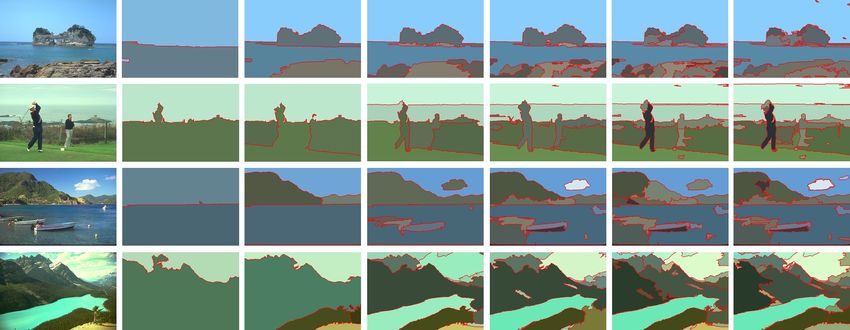
IEEE TRANSACTIONS ON MULTIMEDIA, VOL. 00, NO. 0, * 2021                                                                                              3

                                                                                     Algorithm 1 Subspace Pursuit (SP)
                                                                                     Input: F = [ f 1 , ..., f N ] ∈ Rn×N ; b ∈ Rn ; Lmax = 3; τ =
                                                                                         10−6 ;
                                                                                      1: Initialize j = 0; residual r0 = b; support set T0 = ∅;
                                                                                      2: while krj+1 k2 − krj k2 > τ do
                                                                                           Tt = Tj {i∗ }, where i∗ = maxj {|f T          1
                                                                                                     S
                                                                                      3:                                           j rj | , Lmax };
                                                                                                                 T   1
                                                                                      4:   Tj+1 = maxj {| f Tt b| , Lmax };
                                                                                      5:   rj+1 = (I − PTj+1 )b, where PTj+1 is the projection
                                                                                           onto the span of vectors { f j , j ∈ Tj+1 };
                                                                                      6:   j ← j + 1.
                                                                                      7: end while
                                                                                     Output: c∗ = f T Tj+1 b.

                                                                                     Algorithm 2 Affinity nodes selection (SSC-SP)
                                                                                     Input: F = [ f 1 , ..., f N ] ∈ Rn×N ; Lmax = 3; τ = 10−6 ;
                                                                                      1: Compute c∗j from SP (F−j , f j );
                                                                                              ∗                                 ∗       ∗T
                                                                                      2: Set C = [c∗           ∗
                                                                                                     1 , ..., cN ] and W sp = |C | + |C    |;
                                                                                      3: Compute classification from W sp by spectral clustering.
                                                                                     Output: Affinity nodes.
Fig. 2. An overview of the proposed AF-graph for natural image segmen-
tation. After over-segmenting an input image, we obtain superpixels with
mLab features at different scales. An adjacency-graph is constructed by every
superpixel at each scale. To better reflect the affiliation of superpixels at each   at scale ks with N denoting the superpixel numbers. And
scale, a subspace-preserving representation of them is obtained to further           F = [ f1 , ..., f N ] ∈ Rn×N is denoted as mLab feature matrix
select affinity nodes. The KSC-graph is built upon the selected nodes, and           of the superpixels.
then updated by adjacency-graph across different scales. The final result is
obtained by partitioning the constructed fusion graph through Tcut.
                                                                                     B. Graph construction
                                                                                        For single graph-based image segmentation, a crucial issue
perpixels. The combination of adjacency-graph and adaptive-
                                                                                     is how to approximate each superpixel in the feature space
graph can enrich the property of a fusion graph and further
                                                                                     using a linear combination of its neighboring superpixels.
improve the segmentation performance.
                                                                                     Such an approximation is called as subspace-preserving rep-
                                                                                     resentation between neighboring superpixels, which is calcu-
                               III. M ETHOD                                          lated from the corresponding representation error [7]. Such a
   In this section, we introduce our AF-graph for natural image                      subspace-preserving representation can be formally written as
segmentation. The overview of our framework is shown in                              follows:
Fig. 2. Our AF-graph primarily consists of three components:                                               f j = Fcj , cjj = 0,                (1)
feature representation, graph construction, and graph fusion
                                                                                     where cj ∈ RN is the sparse representation of superpixels, and
and partition.
                                                                                     f j ∈ Rn over the F is a matrix representation of superpixels.
                                                                                     The constraint cjj = 0 prevents the self-representation of f j .
A. Feature representation                                                                For fusion graph-based image segmentation, it is critical
   The main idea of superpixel generation is grouping similar                        to generate the subspace-preserving representation for graph
pixels into perceptually meaningful atomic regions which                             combination. Based on the representation of superpixels, an
always conform well to the local image structures. More                              affinity between every pair nodes is built and further selected
importantly, superpixels generated by different methods with                         through spectral clustering [10]. The selected affinity nodes are
different parameters can capture diverse and multi-scale visual                      used to integrate comprehensively different graphs. Moreover,
contents of an image. We simply over-segment an input image                          due to the linearity of the subspace-preserving representation,
into superpixels by mean shift (MS) [28] and Felzenszwalb-                           segmentation with a linear graph usually results in isolated
Huttenlocher (FH) graph-based method [29] using the same                             regions. In contrast, we propose a KSC-graph to exploit non-
parameters1 (e.g. scale ks = 5) as done by SAS [5]. Then,                            linear structure information. The proposed graph construction
the color features of each superpixel are computed to obtain                         consists of three steps: selecting affinity nodes, constructing
an affinity fusion graph. In our implementation, color feature                       KSC-graph on affinity nodes, and updating KSC-graph.
is formed by mean value in the CIE L*a*b* space (mLab)                                   1) Selecting affinity nodes: As discussed above, affinity
which can approximate human vision and its L component                               nodes are not easily and simply defined because the features of
closely matches the human perception of lightness [7]. We                            multi-scale superpixels change greatly. Although the features
define the superpixels of an input image Ip as Xks = {Xi }N                          vary greatly, the affiliation of multi-scale superpixels may not
                                                            i=1
                                                                                     be changed. It is proved that the affiliation of superpixels
  1 The   parameters of oversegmentation have been discussed in [5] and [6].         can be well approximated by a union of low-dimensional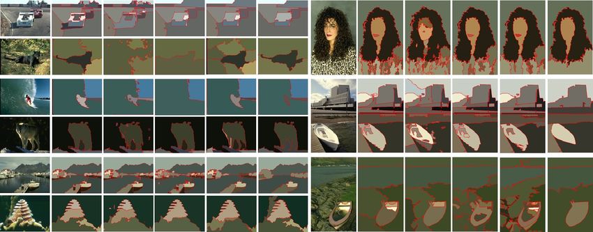
IEEE TRANSACTIONS ON MULTIMEDIA, VOL. 00, NO. 0, * 2021                                                                                          4

                                                                                 linear combination of other superpixels. Therefore, `0 -graph
                                                                                 cannot exploit nonlinear structure information of superpixels.
                                                                                 To discover nonlinear relationships among the selected affinity
                                                                                 nodes, we consider the following problem:

                                                                                   min kX − XZk2F + αkZk1 s.t. ZT 1 = 1, 0 ≤ zij ≤ 1, (3)
                                                                                     Z

                                                                                 where k · k2F represents the squared Frobenius norm, zij is the
                                                                                 (i, j)-th element of similarity graph matrix Z, and α > 0 is a
                                                                                 balance parameter.
                                                                                    It is recognized that nonlinear data can represent linearity
                                                                                 when mapped to an implicit, higher-dimensional space via a
                                                                                 kernel function [31]. All similarities among the superpixels
                                                                                 can be computed exclusively using the kernel function, and
                                                                                 the transformation of superpixels does not need to be known.
                                                                                 Such approach is well-known as the kernel trick, and it greatly
                                                                                 simplifies the computation in kernel space [11] when a kernel
                                                                                 is precomputed. To fully exploit nonlinearity of superpixels,
                                                                                 we define φ : RD → H to be a function mapping superpixels
      (a) Superpixels          (b) SRs                 (c) Areas                 from an input space to a reproducing kernel Hilbert space H,
Fig. 3. Illustration of subspace-preserving representations (SRs) and areas      where DP   ∈ RN ×N is a diagonal matrix with the i-th diagonal
computed by superpixels across different scales. The subspace-preserving
representations of multi-scale superpixels are always sparse. From top to
                                                                                 element j 21 (zij + zji ). The transformation of superpixels X
bottom, the variation of the representations is obviously smaller than that      at a certain scale is φ(X) = {φ(Xi )}Ni=1 . The kernel similarity
of areas with the decreasing number of superpixels. Compared with the            between superpixels Xi and Xj is defined by a predefined
area, the subspace-preserving representation can better reveal the affiliation
of superpixels.                                                                  kernel as KXi ,Xj =< φ(Xi ), φ(Xj ) >. In practice, we use a
                                                                                 linear kernel or Gaussian kernel in our experiments.
                                                                                    This model recovers the linear relationships between su-
subspaces [9]. Therefore, affinity nodes can be classified ac-                   perpixels in the space H and thus the nonlinear relations in
cording to the affiliation of superpixels with subspace approx-                  original representation [31]. So, the problem is formulated as:
imation. This affiliation is considered as subspace-preserving
representation which is obtained by sparse subspace clustering                      min T r(K − 2KZ + ZT KZ) + αkZk1 +βT r(PT LP)
                                                                                         Z                                                     (4)
(SSC). In the SSC, the subspace clustering is implemented by
finding a sparse representation of each superpixel in terms of                                    s.t. ZT 1 = 1, 0 ≤ zij ≤ 1, PT P = I,
other superpixels. In principle, we compute it by solving the
following optimization problem:                                                  where T r(·) is the trace operator, and L is the Laplacian
                                                                                 matrix. β > 0 is also a balance parameter. P ∈ RN ×c is the
          c∗j = arg min kcj k0        s.t. f j = Fcj , cjj = 0,           (2)    indicator matrix. The c elements of i-th row Pi,: ∈ R1×c are
                     cj
                                                                                 used to measure the membership of superpixel Xi belonging
where k · k0 represents the `0 -norm. We solve this problem by                   to c clusters.
subspace pursuit (SP) [30] which is summarized in Algorithm                         We obtain the optimal solution P by c eigenvectors of L
1. The vector c∗j ∈ RN (the j-th column of C∗ ∈ RN ×N ) is                       corresponding to c smallest eigenvalues. When P is fixed, Eq.
computed by SP (F−j , f j ) ∈ RN −1 with a zero inserted in its                  (4) is reformulated column-wisely as:
j-th entry, where F−j is the feature matrix with the j-th column
removed. The SP is subject to a complexity of O(N Lmax ).                                                                              β T
                                                                                             min Kii − 2K i,: Zi + ZT         T
                                                                                                                    i KZi + αZi Zi +    e Zi
   As shown in Fig. 3, we compare the presentations generated                                 Z                                        2 i     (5)
by multi-scale superpixels with their areas across different                                             s.t. ZT
                                                                                                               i 1 = 1, 0 ≤ zij ≤ 1,
scales. It can be seen that the subspace-preserving repre-
sentations of multi-scale superpixels are always sparse. The                     where ei ∈ RN ×1 is a vector with the j-th element eij being
variation of presentations is obviously smaller than that of                     eij = kPi,: − Pj,: k2 . This problem can be solved by many
areas with the decreasing number of superpixels. Compared                        existing quadratic programming in polynomial time. The main
with the area, subspace-preserving representation can better                     computation cost lies in solving Z which is generally solved
reveal the affiliation of superpixels. Based on the presentations,               in parallel. After solving the above problem, we obtain a
the classification of superpixels is obtained by applying our                    symmetric non-negative similarity matrix Z to construct KSC-
proposed SSC-SP. The procedure of affinity node selection                        graph as follows:
(SSC-SP) is summarized in Algorithm 2.
   2) Constructing KSC-graph on affinity nodes: In general,                                                W = (|Z| + |Z|T )/2.                (6)
the basic principle of `0 sparse representation for graph
construction is that each superpixel is approximated with a                      The KSC-graph construction is outlined in Algorithm 3.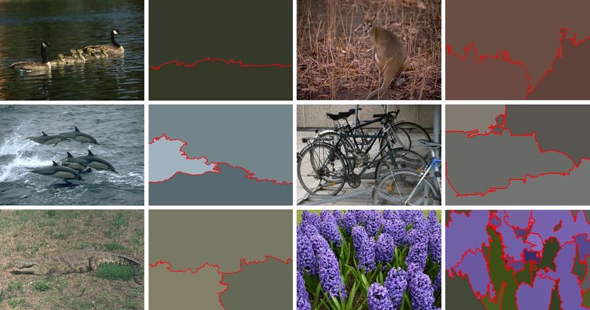
IEEE TRANSACTIONS ON MULTIMEDIA, VOL. 00, NO. 0, * 2021 5
Algorithm 3 KSC-graph construction
Input: Kernel matrix K; α > 0; β > 0; δ = 10−3 ;
1: Initialize random matrix Z and P; j = 0;
kZj+1 −Zj k2
2: while kZj k2 < δ do
3: Update P, which is formed by the c eigenvectors of L =
ZT +Zj
D− j 2 corresponding to the c smallest eigenvectors;
4: For each j, update the j-th column of Zj by solving the
problem Eq. (5).
5: end while
6: Construct KSC-graph W = (|Zj+1 | + |Zj+1 |T )/2
Output: KSC-graph W.
Algorithm 4 Affinity fusion graph-based framework for nat-
ural image segmentation (AF-graph)
Fig. 4. Visual comparison obtained by KSC-graph and `0 -graph. From left to Input: Input image Ip ; parameters α, β; group kT ;
right, superpixel images, KSC-graphs built by the superpixels, segmentation 1: Over-segment an input image Ip to obtain superpixels at
results by the KSC-graphs, `0 -graphs built by the superpixels, segmentation
results by the `0 -graphs are presented, respectively. The KSC-graph produces different scales;
a dense graph, and the `0 -graph is sparser than KSC-graph. The proposed 2: Generate a subspace-preserving representation of color
KSC-graph achieves better performance than `0 -graph. features at each scale to better represent the superpixels
based on the proposed SSC-SP;
3) Updating KSC-graph: Inspired by GL-graph [7], the lo- 3: Select affinity nodes of superpixels based on the proposed
cal neighborhood relationship of superpixels is also considered subspace-preserving representation;
to enrich the property of fusion graph and further improve 4: Construct a KSC-graph on the selected nodes through
segmentation accuracy. As for all superpixels at each scale, kernel spectral clustering;
everyone is connected to its adjacent superpixels, denoted as 5: Construct an adjacency-graph by all superpixels and up-
adjacency-graph A. Let MA be the matrix-representation of all date the KSC-graph at each scale;
adjacent neighbors of every superpixel, we attempt to represent 6: Fuse the updated KSC-graph across different scales and
the f i as a linear combination of elements in MA . In practice, compute to obtain the final segmentation result (pixel-wise
we solve the following optimization problem: labels) through Tcut with group kT ;
Output: Pixel-wise labels.
c˜i = arg min k f i − MA ci k2 . (7)
ci
If a minimizer c˜i has been obtained, the affinity coefficients
Aij between superpixels Xi and Xj are computed as Aij =
We construct a fusion graph to describe the relationships of
1 − 12 (ri,j + rj,i ) with ri,j = k f i − ci,j f j k22 , if i is not equal
pixels to superpixels and superpixels to superpixels, which
to j; Aij = 1 otherwise. For the superpixels at each scale,
aims to enable propagation of grouping cues across superpixels
the KSC-graph W is used to replace the adjacency-graph A to
at different scales. Formally, let G = {U, V, B} denote the fu-
obtain the updated KSC-graph W 0 on affinity nodes.
sion graph with node set U∪V, where U := Ip ∪X = {ui }N U
i=1 ,
To further illustrate the differences between our KSC-graph NV
V := X = {vi }i=1 with NU = |Ip | + |X| and NV = |X|,
and `0 -graph, we use probabilistic rand index (PRI) [32] to
the numbers of nodes in U and V, respectively. The across-
evaluate the results of KSC-graph and `0 -graph on Berkeley AX
Segmentation Database [33]. As shown in Fig. 4, our proposed affinity matrix is defined as B = , where W M S is the
WM S
KSC-graph produces a dense graph, and the `0 -graph is sparser above multi-scale affinity matrix. AX = (aij )|Ip |×|X| are the
than KSC-graph because of its nodes owning fewer neighbors. relationships between pixels and superpixels with aij = 0.001,
The proposed KSC-graph achieves better performance in com- if a pixel i belongs to a superpixel j; aij = 0 otherwise.
parison with `0 -graph.
For the above fusion graph G, the task is to partition it
into kT groups. The kT is a hyper-parameter, which will
C. Graph fusion and partition
be further analyzed in Section IV-B. However, in this case,
To fuse all scales of superpixels, we plug each scale affinity the fusion graph is unbalanced (i.e. NU = NV + |Ip |, and
matrix W 0ks corresponding to its graph into a block diagonal |Ip | >> NV . We have NU >> NV ). We can apply Transfer
multi-scale affinity matrix W M S as follows: cuts (Tcut) algorithm [5] to solve this unbalanced fusion graph.
0 It should be noted that solving the problem takes a complexity
W1 · · · 0
of O(kT |NV |3/2 ) with a constant. The proposed affinity fusion
W M S = ... .. .. . (8)
. . graph-based framework for natural image segmentation is
0
0 ··· W ks summarized in Algorithm 4.
IEEE TRANSACTIONS ON MULTIMEDIA, VOL. 00, NO. 0, * 2021                                                                                                6

                              TABLE I                                                               TABLE III
  Q UANTITATIVE COMPARISON ON BSD300 DATASET FOR DIFFERENT                P ERFORMANCE OF DIFFERENT GRAPHS BEFORE AND AFTER EMBEDDING
  METHODS USING IN THE PROPOSED FRAMEWORK . T HE METHOD IN                INTO THE PROPOSED FRAMEWORK ON BSD300 DATASET. T HE A- GRAPH
  GL- GRAPH [7], k- MEANS , SSC-OMP, AND SSC-SP ARE USED FOR                                 MEANS ADJACENCY- GRAPH .
       SELECTING AFFINITY NODES IN GRAPH CONSTRUCTION .

                                                                             Graphs                                    PRI ↑   VoI ↓   GCE ↓   BDE ↓
       Methods                  PRI ↑     VoI ↓      GCE ↓     BDE ↓
                                                                                            A-graph                    0.84    1.64    0.18    14.73

                                                                             Not embedded
       Ref. [7]                 0.84      1.79       0.19      15.04                        `0 -graph                  0.83    2.08    0.23    14.96
       k-means (k = 2)          0.84      1.69       0.19      14.72                        `1 -graph                  0.80    2.96    0.33    16.08
       SSC-OMP                  0.84      1.65       0.19      14.81                        `2 -graph                  0.80    3.03    0.32    16.33
       SSC-SP                   0.85      1.63       0.18      13.95                        LRR-graph                  0.84    1.74    0.20    15.27
                                                                                            KSC-graph                  0.84    1.74    0.20    15.41

                          TABLE II                                                          A   +   `0 -graph          0.84    1.66    0.19    14.69

                                                                             Embedded
  Q UANTITATIVE COMPARISON ON BSD300 DATASET FOR DIFFERENT                                  A   +   `1 -graph          0.84    1.67    0.19    14.86
          KERNEL FUNCTIONS USING IN OUR FRAMEWORK .                                         A   +   `2 -graph          0.84    1.69    0.19    14.62
                                                                                            A   +   LRR-graph          0.84    1.64    0.18    14.76
    Kernels                       PRI ↑      VoI ↓     GCE ↓     BDE ↓                      A   +   KSC-graph (ours)   0.85    1.63    0.18    13.95
    Linear                         0.85      1.63       0.19      13.95
    Polynomial (a = 0, b = 2)      0.85      1.64       0.18      14.70
    Polynomial (a = 0, b = 4)      0.84      1.64       0.18      14.88   B. Performance analysis
    Polynomial (a = 1, b = 2)      0.84      1.64       0.18      14.92      Selecting affinity nodes. To see how the affinity node
    Polynomial (a = 1, b = 4)      0.85      1.64       0.18      14.57
                                                                          selection is affected by different methods, we compare the
    Gaussian (t = 0.1)             0.84      1.65       0.19      14.90
                                                                          method in GL-graph [7], k-means (k = 2), and SSC-OMP [9]
    Gaussian (t = 1)               0.84      1.68       0.19      14.84
    Gaussian (t = 10)              0.85      1.63       0.18      14.76
                                                                          with our proposed SSC-SP. All parameters of the above
    Gaussian (t = 100)             0.85      1.63       0.18      13.95   algorithms are set to default values. The comparison results
                                                                          on BSD300 dataset are shown in Table I. Obviously, our
                                                                          proposed SSC-SP performs the best on all metrics compared
                                                                          with the method in GL-graph [7], k-means, and SSC-OMP [9].
              IV. E XPERIMENTS AND ANALYSIS
                                                                          Therefore, our subspace-preserving representation which is
   In this section, we first introduce datasets and evaluation            generated by SSC-SP can better reveal the affiliation of multi-
metrics. Then, we show performance analysis about affinity                scale superpixels.
nodes selection, kernel functions, different graph combination,              Kernel function in KSC-graph. To assess the effectiveness
and parameters. Moreover, the results are presented in com-               of different kernel functions in KSC-graph, we adopted 9
parison with the state-of-the-art methods. Finally, we present            different kernels including a linear kernel K(x, y) = xT y, four
time complexity analysis of our AF-graph.                                 polynomial kernels K(x, y) = (a + xT y)b with a ∈ {0, 1} and
                                                                          b ∈ {2, 4}, and four Gaussian kernels K(x, y) = exp(−kx −
                                                                          yk22 /(td2max )) with dmax being the maximal distance be-
A. Datasets and evaluation metrics                                        tween superpixels and t varying in the set {0.1, 1, 10, 100}.
                                                                          Furthermore, all kernels are rescaled to [0, 1] by dividing
   For natural image segmentation, we evaluate the perfor-                each element by the largest pair-wise squared distance. In
mance of our framework on Berkeley segmentation database                  Table II, the Gaussian kernel with t = 100 achieves the best
(BSD) [33] and Microsoft Research Cambridge (MSRC)                        performance on all metrics. We can also observe that our
database [34]. The BSD300 includes 300 images and the                     AF-graph is robust to the kernel functions. Specially, when
ground truth annotations. As an improved version of BSD300,               simply using a linear kernel, our framework can still achieve
the BSD500 contains 500 natural images. The MSRC con-                     a satisfactory performance.
tains 591 images and 23 object classes with accurate pixel-                  Combining different graphs. We construct different basic
wise labeled images. Besides, there are four standard metrics             graphs only using mLab to obtain segmentation results on
which are commonly used for evaluating image segmentation                 BSD300. They are adjacency-graph [5], `0 -graph [6], `1 -
methods: probabilistic rand index (PRI) [32], variation of                graph [10], `2 -graph [37], LRR-graph [38], and our proposed
information (VoI) [35], global consistency error (GCE) [33],              KSC-graph. Then, we employ these basic graphs to construct
and boundary displacement error (BDE) [36]. Among these                   a fusion graph. The parameters in each of these graphs are
metrics, the closer the segmentation result is to the ground-             tuned for the best performance. The segmentation results of
truth, the higher the PRI is, and the smaller the other three             the above graphs are shown in Table III.
measures are. Four metrics of PRI, VoI, GCE, and BDE                         For basic graphs, many works on linear graph partitioning
are computed as the method in [8]. In addition, the average               show that meaningful results are derived from a sparse graph
running time are obtained to evaluate the time complexity of a            such as `0 -graph. The adjacency-graph shows better perfor-
segmentation method. In practice, the best segmentation results           mance for all metrics compared with all single graphs. The
are computed over the value of group kT ranking from 1 to                 main reason is that the LRR-graph often produces a dense
40 as done by GL-graph [7].                                               graph. The `0 -graph performs better than the `1 -graph and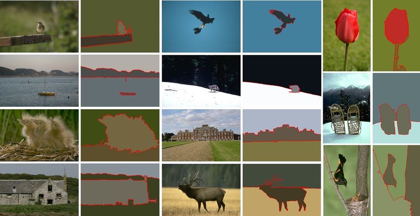
IEEE TRANSACTIONS ON MULTIMEDIA, VOL. 00, NO. 0, * 2021                                                                                                 7

Fig. 5. Visual segmentation examples are obtained by basic graphs in comparison with our proposed AF-graph. From left to right, input images, the
segmentation results of A-graph, `0 -graph, `1 -graph, `2 -graph, KSC-graph, A+`0 -graph, A+`1 -graph, A+`2 -graph, and our AF-graph (A+KSC-graph) are
presented respectively. Our framework can significantly improve the performance of `0 -graph, `1 -graph, and `2 -graph. Our AF-graph can achieve the best
performance for the combination of adjacency-graph and KSC-graph.

                                   (a) PRI                                                                    (b) VoI

                                   (c) GCE                                                                   (d) BDE
Fig. 6. Parameter influence. Each figure is a metric plot when one of the two parameters α and β is fixed. The best performance is obtained when α = 10−5
and β = 10−6 . Our AF-graph is robust to the parameters α and β.

`2 -graph. Because the `0 -graph is sparser than the `1 -graph                in comparison with the basic graphs before and after embedded
and `2 -graph due to the fewer neighbors of its nodes. So,                    into our framework are shown in Fig. 5. Clearly, our AF-graph
the sparsity of a linear graph has a great influence on its                   can achieve the best performance.
segmentation performance. We can also find that our KSC-                         Parameters. To analyze the robustness of our framework,
graph produces a dense graph (in Fig. 4), but its performance                 we study the sensitivity of the two parameters α and β in KSC-
is desirable because of the non-linearity. Our AF-graph is more               graph by fixing one of them to the optimal settings. Parameter
precise for graph combination with respect to all metrics due                 influence on metrics of the KSC-graph is shown in Fig. 6.
to assimilating the advantages of different graphs.                           The best performance is obtained when α = 10−5 and β =
   More importantly, our AF-graph can significantly improve                   10−6 . We can also observe that our AF-graph is robust to the
the performance of these graphs. The metric of PRI has been                   parameters α and β.
enhanced largely and the other three metrics have been greatly                   To explore the influence of group kT to our AF-graph, we
reduced. Some visual segmentation examples of our AF-graph                    show visual results of various kT (kT = 2, 5, 10, 20, 30,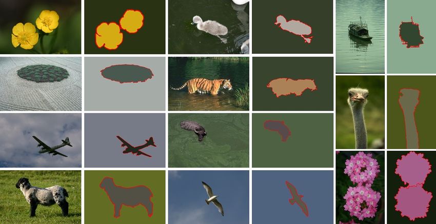
IEEE TRANSACTIONS ON MULTIMEDIA, VOL. 00, NO. 0, * 2021                                                                                                 8

Fig. 7. Visual results are obtained by our AF-graph to explore the influence of kT . From left to right, input images, results of kT = 2, kT = 5, kT = 10,
kT = 20, kT = 30, kT = 40 are presented respectively. When the kT is increased, our AF-graph enforces the global structure over superpixels and masters
the meaning of regions. Moreover, our AF-graph preserves more local information in superpixels.

and 40) in Fig. 7. The results show that visually meaningful                                                    TABLE IV
segmentation can be obtained by carefully tuning of the                            Q UANTITATIVE RESULTS OF THE PROPOSED AF- GRAPH WITH THE
                                                                                       STATE - OF - THE - ART APPROACHES ON BSD300 DATASET.
kT . When the kT is increased, our AF-graph enforces the
global structure over the superpixels and masters the meaning                    Methods                           PRI ↑    VoI ↓    GCE ↓      BDE ↓
of regions. Moreover, our AF-graph preserves more local
                                                                                 Ncut [12]                          0.72     2.91      0.22     17.15
information in superpixels.
                                                                                 FCM [15]                           0.74     2.87      0.41     13.78
                                                                                 MNCut [13]                         0.76     2.47      0.19     15.10
C. Comparison with the state-of-the-art methods                                  SuperParsing [23]                  0.76     2.04      0.28     15.05
   To verify our framework, we report the quantitative re-                       HIS-FEM [14]                       0.78     2.31      0.22     10.66
sults in comparison with the state-of-the-art methods in Ta-                     SFFCM [15]                         0.78     2.02      0.26     12.90
bles IV∼VI. Specially, we highlight in bold the best re-                         Context-sensitive [24]             0.79     3.92      0.42      9.90
                                                                                 CCP [17]                           0.80     2.47      0.13     11.29
sult for each qualitative metric. The above compared meth-
                                                                                 H +R Better [18]                   0.81     1.83      0.21     12.16
ods include: FH [29], MS [28], Ncut [12], MNcut [13],                            Corr-Cluster [25]                  0.81     1.83        –      11.19
CCP [17], Context-sensitive [24], Corr-Cluster [25], Super-                      RIS+HL [39]                        0.81     1.82      0.18     13.07
Parsing [23], HIS-FEM [14], Sobel-AMR-SC [16], Heuristic                         HO-CC [26]                         0.81     1.74        –      10.38
better and random better (H +R Better) [18], TPG [27], HO-                       TPG [27]                           0.82     1.77        –        –
CC [26], SAS [5], `0 -graph [6], GL-graph [7], FNCut [22],                       SAS [5]                            0.83     1.65      0.18     11.29
Link MS+RAG+GLA [19], SFFCM [15], gPb-owt-ucm [20],                              `0 -graph [6]                      0.84     1.99      0.23     11.19
RIS+HL [39], MMGR-AFCF [40], and AASP-graph [8]. For                             GL-graph [7]                       0.84     1.80      0.19     10.66
fair comparison, the quantitative results are collected from                     AASP-graph [8]                     0.84     1.65      0.17     14.64
                                                                                 CCP-LAS [17]                       0.84     1.59      0.16     10.46
their evaluations reported in publications.
                                                                                 AF-graph (Linear)                  0.85     1.63      0.19     13.95
   As shown in Table IV, our AF-graph ranks the first in                         AF-graph (Gaussian, t = 100)       0.85     1.63      0.18     13.95
PRI and second in VoI on BSD300 dataset. In Table V, our
framework achieves the best result in PRI, VoI and GCE on
BSD500 dataset. In Table VI, our AF-graph ranks the first
in PRI, VoI, and GCE on MSRC dataset. To demonstrate                          performance due to the integration of the contour and color
the advantages of our AF-graph in practical applications,                     cues of segmenting images. In contrast, our framework only
we present visual segmentation results with kT = 2 and 3,                     utilizes the color information. Moreover, the BDE of our
respectively. From the Fig. 8, we observe that our framework                  framework is unsatisfied. The failure examples by AF-graph
can be used to segment the salient objects in the following                   are shown in Fig. 9. When the detected object is too tiny,
cases: i) the detected object is tiny, such as the airplane, wolf,            and its texture is easily to be confused with background, our
buffalo, and trawler; ii) multiple objects are needed to be                   framework cannot achieve accurate segmentation. The main
segmented in the same image, such as flower, eagle, boat, and                 reason is that our AF-graph only uses pixel color information,
bird; iii) the color of both background and object are quite                  which fails to capture enough contour and texture cues of
similar, such as nestling, ostrich, and house.                                segmenting images.
   It should be noted that the CCP-LAS (CCP [17] based on                        Especially, our AF-graph follows a similar, but not identical
layer-affinity by SAS [5]) approach has the most competitive                  strategy as the SAS, `0 -graph, GL-graph, and AASP-graph.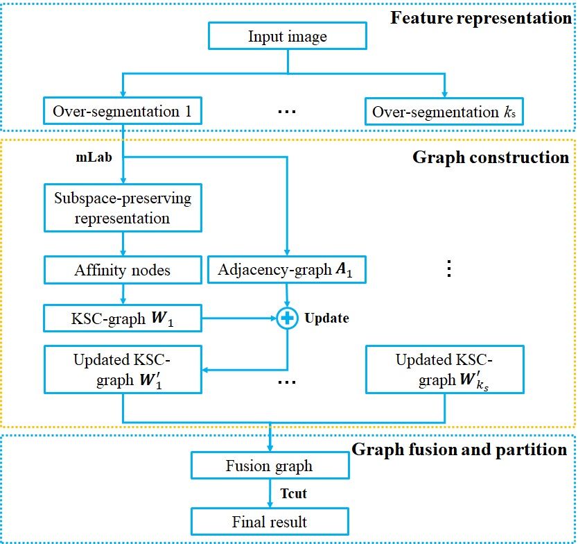
IEEE TRANSACTIONS ON MULTIMEDIA, VOL. 00, NO. 0, * 2021 9
TABLE V
Q UANTITATIVE RESULTS OF THE PROPOSED AF- GRAPH WITH THE
STATE - OF - THE - ART APPROACHES ON BSD500 DATASET.
Methods PRI ↑ VoI ↓ GCE ↓ BDE ↓
FCM [15] 0.74 2.88 0.40 13.48
MNCut [13] 0.76 2.33 – –
MMGR-AFCF [40] 0.76 2.05 0.22 12.95
SFFCM [15] 0.78 2.06 0.26 12.80
FH [29] 0.79 2.16 – –
MS [28] 0.79 1.85 0.26 –
Link MS+RAG+GLA [19] 0.81 1.98 – – (a) kT = 2
FNCut [22] 0.81 1.86 – –
Sobel-AMR-SC [16] 0.82 1.77 – –
HO-CC [26] 0.83 1.79 – 9.77
SAS [5] 0.83 1.70 0.18 11.97
gPb-owt-ucm [20] 0.83 1.69 – 10.00
`0 -Graph [6] 0.84 2.08 0.23 11.07
AF-graph (Linear) 0.84 1.67 0.18 13.63
AF-graph (Gaussian, t = 100) 0.84 1.68 0.19 13.91
TABLE VI
Q UANTITATIVE RESULTS OF THE PROPOSED AF- GRAPH WITH THE
STATE - OF - THE - ART APPROACHES ON MSRC DATASET. (b) kT = 3
Fig. 8. Visual segmentation results of our AF-graph. All images are segmented
Methods PRI ↑ VoI ↓ GCE ↓ BDE ↓ into 2 and 3 regions, namely kT is set to 2 and 3 in Tcut, respectively. Note
that salient objects and multiple objects can be segmented accurately.
gPb-Hoiem [20] 0.61 2.85 – 13.53
MNCut [13] 0.63 2.77 – 11.94
SuperParsing [23] 0.71 1.40 – –
SFFCM [15] 0.73 1.58 0.25 12.49
Corr-Cluster [25] 0.77 1.65 – 9.19
gPb-owt-ucm [20] 0.78 1.68 – 9.80
HO-CC [26] 0.78 1.59 – 9.04
RIS+HL [39] 0.78 1.29 – –
SAS [5] 0.80 1.39 – –
`0 -graph [6] 0.82 1.29 0.15 9.36
AF-graph (Linear) 0.83 1.24 0.14 13.33
AF-graph (Gaussian, t = 100) 0.82 1.23 0.14 13.76
Fig. 9. Failure examples by AF-graph. Our AF-graph only uses pixel color
information, which fails to capture enough contour and texture cues of
Different from SAS only using adjacent neighborhoods of segmenting images.
superpixels and `0 -graph only using `0 affinity graph of
superpixels, our AF-graph can combine different basic graphs.
It allows the AF-graph to have a long-range neighborhood The main reason is that our AF-graph selects affinity nodes in
topology with a high discriminating power and nonlinearity. an exact way. In particular, our AF-graph achieves the correct
The main differences among GL-graph, AASP-graph and our and accurate segmentation even in the difficult cases compared
method are the way of graph construction and their fusion with the other similar methods. These cases are: i) the detected
principle. In GL-graph, the superpixels are simply classified object is highly textured, and the background may be highly
into three sets according to their areas. In AASP-graph, the unstructured (e.g. curler, coral, and panther); ii) objects of the
superpixels are classified into two sets based on affinity same type appear in a large, fractured area of the image (e.g.
propagation clustering. In our AF-graph, different basic graphs racecars and boat).
are fused by affinity nodes which are selected by the proposed
SSC-SP. Moreover, a novel KSC-graph is built upon these D. Time complexity analysis
affinity nodes to explore the nonlinear relationships, and then Our framework includes the steps of feature representation,
the adjacency-graph of all superpixels is used to update the graph construction, and graph fusion and partition. Time
KSC-graph. complexities of SP, KSC-graph construction, Tcut for graph
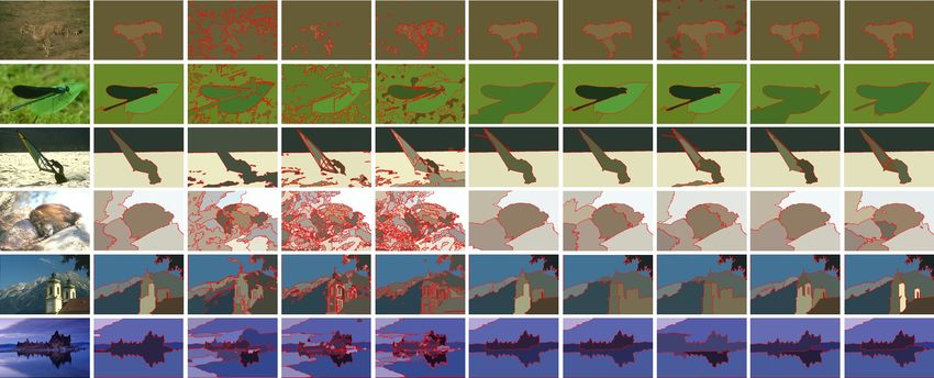
Moreover, various results of the SAS, `0 -graph, GL-graph, partition are analyzed in Section III-B and Section III-C
AASP-graph, and our AF-graph are shown in Fig. 10, respec- respectively. For each phase, it costs 5.11 seconds to generate
tively. It shows that our framework achieves a desirable result superpixels and extract features, 1.65 seconds for affinity
with less tuning for kT in Tcut (e.g. for surfers, kT = 3). nodes selection, 1.68 seconds to build fusion graph, and only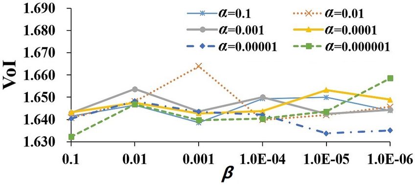
IEEE TRANSACTIONS ON MULTIMEDIA, VOL. 00, NO. 0, * 2021                                                                                                        10

Fig. 10. Visual comparison on BSD dataset are obtained by SAS, `0 -graph, GL-graph, AASP-graph, and our AF-graph. Two columns of the comparison
results are shown here. From left to right, input images, the results of the SAS, `0 -graph, GL-graph, AASP-graph, and our AF-graph are presented respectively.

0.82 seconds for graph partition. Our AF-graph takes totally                      [4] X. Li, L. Jin, E. Song, and Z. He, “An integrated similarity metric for
9.26 seconds to segment an image with the size of 481×321                             graph-based color image segmentation,” Multimedia Tools Application,
                                                                                      vol. 75, no. 6, pp. 2969–2987, 2016.
pixels from BSD on average, which is slower than SAS with                         [5] Z. Li, X. Wu, and S. Chang, “Segmentation using superpixels: A
7.44 seconds. In contrast, AASP-graph takes more than 15                              bipartite graph partitioning approach,” in IEEE Conference on Computer
seconds in which the global nodes selection and `0 -graph con-                        Vision and Pattern Recognition, 2012, pp. 789–796.
                                                                                  [6] X. Wang, H. Li, C. Bichot, S. Masnou, and L. Chen, “A graph-cut
struction cost much more time than our AF-graph. Moreover,                            approach to image segmentation using an affinity graph based on `0 -
`0 -graph, MNcut, CCP-LAS, GL-graph, and Ncut usually take                            sparse representation of features,” in IEEE International Conference on
more than 20, 30, 40, 100, and 150 seconds, respectively. The                         Image Processing, 2013, pp. 4019–4023.
main reason is that extracting various features cost too much                     [7] X. Wang, Y. Tang, S. Masnou, and L. Chen, “A global/local affinity
                                                                                      graph for image segmentation,” IEEE Transactions on Image Processing,
computational time. All experiments are conducted under the                           vol. 24, no. 4, pp. 1399–1411, 2015.
PC condition of 3.40GHz of Intel Xeon E5-2643 v4 processor,                       [8] Y. Zhang, H. Zhang, Y. Guo, K. Lin, and J. He, “An adaptive affinity
64G RAM, and Matlab 2018a.                                                            graph with subspace pursuit for natural image segmentation,” in IEEE
                                                                                      International Conference on Multimedia and Expo, 2019, pp. 802–807.
                                                                                  [9] C. You, D. P. Robinson, and R. Vidal, “Scalable sparse subspace
             V. C ONCLUSION AND FUTURE WORKS                                          clustering by orthogonal matching pursuit,” in IEEE Conference on
                                                                                      Computer Vision and Pattern Recognition, 2016, pp. 3918–3927.
   In this paper, our AF-graph combines adjacency-graphs and                     [10] E. Elhamifar and R. Vidal, “Sparse subspace clustering: Algorithm,
KSC-graphs by affinity nodes of multi-scale superpixels to                            theory, and applications,” IEEE Transactions on Pattern Analysis and
                                                                                      Machine Intelligence, vol. 35, no. 11, pp. 2765–2781, 2013.
obtain a better segmentation result. These affinity nodes are                    [11] C. Zhang, F. Nie, and S. Xiang, “A general kernelization framework for
selected by our proposed SSC-SP and further used to construct                         learning algorithms based on kernel PCA,” Neurocomputing, vol. 73,
a KSC-graph. The proposed KSC-graph is then updated by an                             no. 4, p. 959–967, 2010.
                                                                                 [12] J. Shi and J. Malik, “Normalized cuts and image segmentation,” IEEE
adjacency-graph of all superpixels at each scale. Experimental                        Transactions on Pattern Analysis and Machine Intelligence, vol. 22, pp.
results show the good performance and high efficiency of the                          888–905, 2000.
proposed AF-graph. We also compare our framework with                            [13] T. Cour, F. Benezit, and J. Shi, “Spectral segmentation with multiscale
the state-of-the-art approaches, and our AF-graph achieves                            graph decomposition,” in IEEE Conference on Computer Vision and
                                                                                      Pattern Recognition, 2005, pp. 1124–1131.
competitive results on BSD300, BSD500 and MSRC datasets.                         [14] S. Yin, Y. Qian, and M. Gong, “Unsupervised hierarchical image
In the future, we will explore the combination of graph and                           segmentation through fuzzy entropy maximization,” Pattern Recognition,
deep unsupervised learning to improve image segmentation                              vol. 68, p. 245–259, 2017.
                                                                                 [15] T. Lei, X. Jia, Y. Zhang, S. Liu, H. Meng, and A. K. Nandi, “Superpixel-
performance.                                                                          based fast fuzzy c-means clustering for color image segmentation,” IEEE
                                                                                      Transactions on Fuzzy Systems, vol. 27, no. 9, pp. 1753–1766, 2019.
                                                                                 [16] T. Lei, X. Jia, T. Liu, S. Liu, H. Meng, and A. K. Nandi, “Adaptive
                              R EFERENCES                                             morphological reconstruction for seeded image segmentation,” IEEE
 [1] C. Fang, Z. Liao, and Y. Yu, “Piecewise flat embedding for image                 Transactions on Image Processing, vol. 28, no. 11, pp. 5510–5523, 2019.
     segmentation,” IEEE Transactions on Pattern Analysis and Machine            [17] X. Fu, C. Wang, C. Chen, C. Wang, and C.-J. Kuo, “Robust image
     Intelligence, vol. 41, no. 6, pp. 1470–1485, 2019.                               segmentation using contour-guided color palettes,” in IEEE International
 [2] M. Pereyra and S. McLaughlin, “Fast unsupervised bayesian image                  Conference on Computer Vision, 2015, pp. 1618–1625.
     segmentation with adaptive spatial regularisation,” IEEE Transactions       [18] K. Li, W. Tao, X. Liu, and L. Liu, “Iterative image segmentation with
     on Image Processing, vol. 26, pp. 2577–2587, 2017.                               feature driven heuristic four-color labeling,” Pattern Recognition, vol. 76,
 [3] R. Hettiarachchi and J. Peters, “Voronoi region-based adaptive unsu-             pp. 69–79, 2018.
     pervised color image segmentation,” Pattern Recognition, vol. 65, pp.       [19] H. Cho, S. Kang, and Y. H. Kim, “Image segmentation using linked
     119–135, 2016.                                                                   mean-shift vectors and global/local attributes,” IEEE Transactions on
IEEE TRANSACTIONS ON MULTIMEDIA, VOL. 00, NO. 0, * 2021 11
Circuits and Systerms for Video Technology, vol. 27, no. 10, pp. 2132–
2140, 2017.
[20] A. Pablo, M. Michael, F. Charless, and M. Jitendra, “Contour detection
and hierarchical image segmentation,” IEEE Transactions on Pattern
Analysis and Machine Intelligence, vol. 33, no. 5, pp. 898–916, 2011.
[21] T. Wang, J. Yang, Z. Ji, and Q. Sun, “Probabilistic diffusion for inter-
active image segmentation,” IEEE Transactions on Image Processing,
vol. 28, no. 1, pp. 330–342, 2019.
[22] T. H. Kim, K. M. Lee, and S. U. Lee, “Learning full pairwise affinities
for spectral segmentation,” IEEE Transactions on Pattern Analysis and
Machine Intelligence, vol. 35, no. 7, pp. 1690–1703, July 2013.
[23] J. Tighe and S. Lazebnik, “Superparsing: Scalable nonparametric image
parsing with superpixels,” in European Conference on Computer Vision,
2010.
[24] X. Bai, X. Yang, L. J. Latecki, W. Liu, and Z. Tu, “Learning context-
sensitive shape similarity by graph transduction,” IEEE Transactions on
Pattern Analysis and Machine Intelligence, vol. 32, no. 5, pp. 861–874,
May 2010.
[25] S. Kim, S. Nowozin, P. Kohli, and C. D. Yoo, “Task-specific image
partitioning.” IEEE Transactions on Image Processing, vol. 22, no. 2,
pp. 488–500, 2013.
[26] S. Kim, C. D. Yoo, S. Nowozin, and P. Kohli, “Image segmentation
using higher-order correlation clustering,” IEEE Transactions on Pattern
Analysis and Machine Intelligence, vol. 36, no. 9, pp. 1761–1774, 2014.
[27] X. Yang, L. Prasad, and L. J. Latecki, “Affinity learning with diffusion
on tensor product graph,” IEEE Transactions on Pattern Analysis and
Machine Intelligence, vol. 35, no. 1, pp. 28–38, 2013.
[28] D. Comaniciu and P. Meer, “Mean shift: a robust approach toward
feature space analysis,” IEEE Transactions on Pattern Analysis and
Machine Intelligence, vol. 24, no. 5, pp. 603–619, 2002.
[29] P. F. Felzenszwalb and D. P. Huttenlocher, “Efficient graph-based image
segmentation,” International Journal of Computer Vision, vol. 59, no. 2,
pp. 167–181, 2004.
[30] W. Dai and O. Milenkovic, “Subspace pursuit for compressive sens-
ing signal reconstruction,” IEEE Transactions on Information Theory,
vol. 55, no. 5, pp. 2230–2249, 2009.
[31] Z. Kang, C. Peng, and Q. Cheng, “Twin learning for similarity and
clustering: A unified kernel approach,” in AAAI Conference on Artificial
Intelligence, 2017, pp. 2080–2086.
[32] R. Unnikrishnan, C. Pantofaru, and M. Hebert, “Toward objective
evaluation of image segmentation algorithms,” IEEE Transactions on
Pattern Analysis and Machine Intelligence, vol. 29, no. 6, pp. 929–944,
2007.
[33] D. R. Martin, C. Fowlkes, D. Tal, and J. Malik, “A database of human
segmented natural images and its application to evaluating segmentation
algorithms and measuring ecological statistics,” in IEEE International
Conference on Computer Vision, 2001, pp. 416–423.
[34] J. Shotton, J. Winn, C. Rother, and A. Criminisi, “Textonboost: Joint
appearance, shape and context modeling for multi-class object recogni-
tion and segmentation,” in European Conference on Computer Vision,
2006, pp. 1–5.
[35] M. Meilă, “Comparing clusterings–an information based distance,” Jour-
nal of Multivariate Analysis, vol. 98, no. 5, pp. 873–895, May 2007.
[36] J. Freixenet, X. Muñoz, D. Raba, J. Martı́, and X. Cufı́, “Yet another
survey on image segmentation: Region and boundary information inte-
gration,” in European Conference on Computer Vision, 2002, pp. 408–
422.
[37] X. Peng, Z. Yu, Z. Yi, and H. Tang, “Constructing the L2-graph for
robust subspace learning and subspace clustering,” IEEE Transactions
on Cybernetics, vol. 47, no. 4, pp. 1053–1066, 2017.
[38] G. Liu, Z. Lin, S. Yan, J. Sun, Y. Yu, and Y. Ma, “Robust recovery of
subspace structures by low-rank representation,” IEEE Transactions on
Pattern Analysis and Machine Intelligence, vol. 35, no. 1, pp. 171–184,
2013.
[39] J. Wu, J. Zhu, and Z. Tu, “Reverse image segmentation: A high-level
solution to a low-level task,” in British Machine Vision Conference,
2014.
[40] T. Lei, P. Liu, X. Jia, X. Zhang, H. Meng, and A. K. Nandi, “Automatic
fuzzy clustering framework for image segmentation,” IEEE Transactions
on Fuzzy Systems, 2019.You can also read