ALB Risk version 1.1: Asian Longhorned Beetle Dispersal Risk Estimation Tool - USDA ...
←
→
Page content transcription
If your browser does not render page correctly, please read the page content below
Forest Service
                       U.S. DEPARTMENT OF AGRICULTURE

Northern Research Station                 General Technical Report NRS-201   April 2021

ALB Risk version 1.1: Asian Longhorned Beetle
Dispersal Risk Estimation Tool
R. Talbot Trotter III, Melissa L. Warden, Scott Pfister,
Ryan J. Vazquez, Josie K. Ryan, and Michael Bohne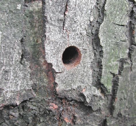
Abstract
The Asian longhorned beetle (Anoplophora glabripennis Motschulsky) is an invasive polyphagous
woodborer that has been introduced to North America and Europe. Due to the severe economic
and ecological damage resulting from infestations of this insect, many countries, including the
United States, have adopted policies of eradication. However, managing eradication can be a
daunting challenge as it requires program managers to identify and destroy individual infested
trees distributed across landscapes that may include millions of host trees. This report describes
the use of the computer software program ALB Risk version 1.1, which estimates the boundaries
of the at-risk landscape, as well as the distribution of risk within the infestation based on
dispersal patterns. The program generates risk-maps, identifies priority areas for management,
and estimates the potential return on survey effort. The software is available at https://doi.
org/10.2737/NRS-GTR-201.

The Authors
R. TALBOT TROTTER III is a research ecologist with the USDA Forest Service in Hamden, CT.
MELISSA L. WARDEN is a quantitative analyst with USDA Animal and Plant Health Inspection
Service, Plant Protection and Quarantine, Science and Technology in Buzzards Bay, MA.
SCOTT PFISTER is the Director of the Otis Laboratory with the USDA Animal and Plant Health
Inspection Service, Plant Protection and Quarantine, Science and Technology in Buzzards Bay, MA.
RYAN J. VAZQUEZ is the Director for the Massachusetts Asian Longhorned Beetle Cooperative
Eradication Program with the USDA Animal and Plant Health Inspection Service, Plant Protection
and Quarantine in Worcester, MA.
JOSIE K. RYAN is a national operations manager for the Asian Longhorned Beetle Eradication
Program with USDA Animal and Plant Health Inspection Service, Plant Protection and Quarantine
in Amityville, NY.
MICHAEL BOHNE is a forest health group leader with the USDA Forest Service, Durham, NH.

Manuscript received for publication 27 April 2020

Published by
U.S. FOREST SERVICE
ONE GIFFORD PINCHOT DRIVE
MADISON, WI 53726
April 2021
CONTENTS
Executive Summary..................................................................................................................................... iv
Introduction
      A History of the Asian Longhorned Beetle in the United States............................................. 1
      Asian Longhorned Beetle Eradication Strategies and Tools..................................................... 3
      Ongoing Needs to Estimate Risk, Optimize Surveys, and Track Eradication Progress.... 5
ALB Risk version 1.1....................................................................................................................................... 6
      Software Summary, Structure, and Assumptions........................................................................ 6
ALB Risk version 1.1: Software User Guide............................................................................................. 8
      Downloading, Installing, and Starting ALB Risk version 1.1...................................................... 8
      Using the Provided Example Data as Model Input.................................................................... 11
      Using User-Provided Data as Model Input................................................................................... 12
      Analysis Settings and Options.......................................................................................................... 13
      Evaluating the Output......................................................................................................................... 21
      Output Data and Mapping the Results.........................................................................................25
      Errors, Bugs, and Other Problems................................................................................................... 26
Acknowledgments...................................................................................................................................... 26
Literature Cited............................................................................................................................................. 27
EXECUTIVE SUMMARY
The Asian longhorned beetle (Anoplophora glabripennis Motschulsky) is an invasive polyphagous
woodborer which has been introduced to North America and Europe via the transportation of infested
solid wood packing material. The ubiquitous use of wood packaging (such as pallets and crates) and
containerized freight has facilitated the establishment of breeding populations in forested and urban
landscapes in at least 11 countries. Due to the substantial economic and ecological damage resulting
from infestations, many countries including the United States have adopted policies of eradication.
However, managing eradication can be a daunting challenge as it requires program managers to
identify each infested tree on the landscape and destroy it by felling and chipping. Because locations
with beetle populations can include forested, urban, peri-urban, and agricultural landscapes with
millions of individual host trees, tools that accelerate survey progress by identifying areas with high
risk are needed. This tool seeks to address these needs.

The purpose of the computer software program ALB Risk v1.1 is to estimate the distribution of risk
within an area infested by the Asian longhorned beetle based on dispersal patterns specific to that
infested area and the locations and infestation levels of known infested trees. The process includes four
steps used to produce risk-maps, identify priority areas for management, and estimate the potential
return on survey effort. These steps are based on the computation methods described in Trotter and
Hull-Sanders (2015) and Trotter et al. (2018) which have been expanded to include additional output
that may be of use to eradication management programs. Briefly summarized, these four steps are:

    1) Reconstruct patterns of beetle dispersal by connecting the infested trees on the landscape. The
       connections among the infested trees are determined using a set of rules based on the biology
       and behavior of the beetle. These rules can be modified by the user to account for knowledge
       gaps and to incorporate new knowledge about beetle behavior as it becomes available.
    2) Use the reconstructed pattern of beetle dispersal from Step 1 to estimate the probability
       distributions for beetle dispersal to include both distance and direction. These probabilities are
       commonly called dispersal kernels. These three-factor (direction, distance, and probability)
       dispersal kernels are unique to each infested region.
    3) The dispersal probabilities (kernels) are applied to the locations of each known infested tree
       to estimate the risk of beetle dispersal around that tree. This process is repeated for each
       known infested tree on the landscape and the overall probability that at least one beetle has
       arrived from at least one infested tree on the landscape is calculated for each location on the
       landscape. The default settings produce estimates on a hectare-by-hectare basis.
    4) The distribution of risk on the landscape is output as a map and GIS data layer, and used
       to identify a) the sequence of locations to manage to maximize eradication progress, b) the
       portion of the infested landscape to manage to achieve a given probability of eradication,
       and c) an effort/benefit curve describing the nonlinear relationship between the total area
       managed and the overall probability of eradication.

The output maps and graphics produced by ALB Risk version 1.1 can be used to assess landscape
patterns of ALB dispersal, the distribution of dispersal risk, and the relationship between survey effort
and eradication success. These outputs can also be used as the input required to run a second tool
called ALB Dynamic Risk version 1.0.1 This tool provides dynamic estimates of risk on the landscape
based the history of eradication program activities including the timing, location, intensity, frequency,
and method of surveys.

1
 For additional information and access to the model and documentation, contact Talbot Trotter at
Robert.T.Trotter@usda.gov.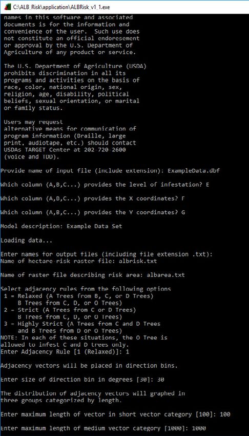
INTRODUCTION
A History of the Asian Longhorned Beetle in the United States
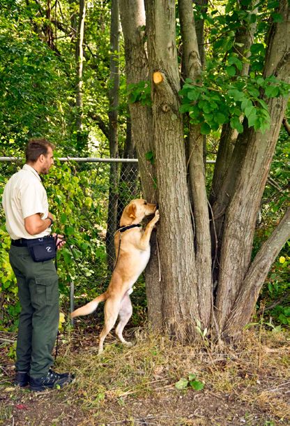
In August of 1996, a resident in New York City noticed
damage to several Norway maple (Acer platanoides)
trees along a street in the Greenpoint neighborhood of
Brooklyn (Haack et al. 1997). The trunks and branches
of the trees had round holes roughly one-half inch in
diameter with small piles of sawdust below, as though
the trees had been vandalized by someone using a hand
drill (Fig. 1). The resident reported the damage to New
York City Parks and Recreation, and within days city
and state foresters had collected several large beetles
from the damaged trees (Fig. 2). Rapid efforts by city
and state foresters, the U.S. Department of Agriculture,
and entomologists at Cornell University confirmed the
identity of the beetles, and the first infestation of the
Asian longhorned beetle (Anoplophora glabripennis
Motschulsky; ALB) in North America was discovered.
Figure 1.—When adult Asian longhorned beetles emerge
Within weeks the U.S. Department of Agriculture
from a tree, they leave distinctive exit holes, which are round
(USDA) Animal and Plant Health Inspection Service and approximately one-half inch in diameter. Courtesy photo
(APHIS) had federal staff in New York City working by Pennsylvania Department of Conservation and Natural
with state and city agencies to determine the size of Resources – Forestry/Bugwood.org.
the infestation and to begin the process of eradicating
it. The rapid and aggressive response to this beetle
by city, state, and federal land managers was driven
by knowledge that the Asian longhorned beetle had
already caused significant damage to North American
tree species that had been planted in China to help slow
desertification.
In 1978 the Chinese government initiated the
Three North Forest Protection Program, a massive
reforestation and afforestation effort intended to slow
the expansion of the Gobi Desert, reduce dust storms,
and provide wood resources to local populations. As
of 2003 the program had carried out afforestation
work on more than 150 million hectares of farmland Figure 2.—Adult Asian longhorned beetles on a branch.
and grasslands (Qui et al. 2017). Many of the planted The beetle on the bottom is a female and the beetle above
is a male. Note the male’s antennae are substantially longer
trees were North American poplars and poplar hybrids than its body. The beetles are black with white spots, often
selected for their rapid growth and soil tolerance about 1.5 inches long not including the antennae, and on
characteristics. Unfortunately, many of the species and close inspection, often have blue feet. USDA APHIS photo by
hybrids that were planted were highly susceptible to Kenneth R. Law.
attack by the native Asian longhorned beetle, leading to
an infestation spanning a large portion of China. use in high value applications such as furniture, veneer,
or dimensional lumber. To recover some value from
When beetles infest trees, the larvae bore through the the timber this low-quality wood is commonly used in
phloem and xylem leaving tunnels up to one-half inch commodities such as pallets, crates, and dunnage where
in diameter in the lumber. These holes and galleries the quality or appearance of the wood is not critical.
reduce the wood’s quality and make it unsuitable for These solid wood packing materials are heavily used
1
in international shipping (Fig. 3), and moving infested
material provides an opportunity for larvae living in
the wood to be transported internationally (Haack et al.
1997) and emerge to infest new environments.

In 1992, Asian longhorned beetles were found in
warehouses and ports of entry in North America
(Haack et al. 2010) demonstrating the potential for
this damaging pest to be moved to novel landscapes,
including North America. By 1998, beetles had been
detected at more than 30 warehouses and ports of entry.
These detections, combined with the susceptibility of
                                                           Figure 3.—Solid wood packing material, such as these crates
North American tree species to infestation, made the       and pallets, are the primary path for beetles to move from
Asian longhorned beetle a species of high concern.         their native range in China and the Korean Peninsula, or from
                                                           other established infestations, to other parts of the world.
With the detection of a breeding population of the         USDA APHIS photo/Bugwood.org.
beetles in New York City, APHIS and the USDA Forest
Service (USDA FS) conducted a rapid risk assessment        made a “Declaration of Emergency Because of the
to evaluate the threat ALB might pose to North             Asian Longhorned Beetle” (64 CFR 12800-12801) to
American trees and forests. The analyses confirmed the     accelerate efforts to find, quarantine, and eradicate
beetle would likely cause significant damage to lumber     this species in the United States. Since the discovery of
production, ecotourism, maple syrup production,            Asian longhorned beetles in New York City, breeding
public and private lands management, and property          populations have been found in Illinois, Massachusetts,
values (Kucera 1996). Adding urgency to the situation,     New York, New Jersey, and Ohio.
a study by Nowak et al. (2001) found that within the
United States, 1.2 billion urban trees (representing       ALB has a broad host range that includes tree species
about 30 percent of the urban tree cover), with an         from at least 15 families, including the abundant
estimated value of $669 billion, would be at risk if the   and widely distributed genera Acer (maple), Populus
beetle were to permanently establish and spread. In        (cottonwood, poplar, and aspen), Salix (willow),
response to these ecological and economic threats,         and Ulmus (elm) (Fig. 4). In addition to the United
the Secretary of the U.S. Department of Agriculture        States, breeding populations of the beetle have been

                                                                          Figure 4.—An analysis by Kappel et al.
                                                                          (2017) shows the broad geographic
                                                                          range of suitable host trees and the
                                                                          size of the landscape threatened by
                                                                          the Asian longhorned beetle. Courtesy
                                                                          image from Kappel et al 2017, used
                                                                          with permission.

                                                                                                                           2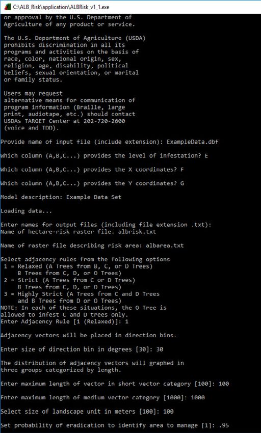
found in Austria, Belgium, Canada, Finland, France,         and manage it have been discussed in greater detail in
Germany, Italy, Turkey, the Netherlands, and the            numerous sources (e.g., Hsiao 1982, Meng et al. 2015)
United Kingdom. The threat posed by the beetle has          and so we do not seek here to provide a comprehensive
prompted Canada, the United States, and members             review. Rather, we provide brief descriptions of
of the European and Mediterranean Plant Protection          eradication tools for the convenience of the reader,
Organization (EPPO) to adopt ISPM-152 to reduce the         and to place the utility of the software described in this
risk of introducing the beetle to new locations. Further,   document in a broader eradication-strategy context.
these countries have established policies of eradication
when infestations are found, and in some locations,         Traps: For some notable
eradication has been achieved.                              invasive species, such as
                                                            the gypsy moth (Lymantria
In the United States, the federal government has            dispar dispar Linnaeus),
spent approximately $750 million on eradication             pheromone-baited traps
programs (a value that represents about 0.1 percent         have provided a highly
of the expected cost to cities in the United States         effective survey tool for
should the beetle become widely established). As a          documenting the presence,
result of these efforts, the beetle has been eradicated     abundance, and distribution
from New Jersey, Chicago, Boston, and in the New            of the insect (Fig. 5).
York City metropolitan areas of Manhattan, Staten           Trapping surveys have
Island, Queens, Brooklyn, and the town Islip on             several advantages including
Long Island. However, about 220 square miles (110           the potential to effectively
in Worcester, MA; 57 in Bethel, OH; and 53 on Long          sample large areas, the
Island) remain under quarantine as of the end of            potential for high species
2019, and in the spring of 2020 a new infestation was       specificity, and the effective
detected in South Carolina. Eradication programs in         deployment and monitoring
these areas are tasked with eliminating the infestations    of traps without the need
from complex urban, rural, agricultural, and forested       for specialized training.
landscapes. Though past eradication programs have           With these advantages              Figure 5.—A panel intercept trap is
                                                                                               used to survey for Asian longhorned
been successful, there remain opportunities for             in mind, multiple efforts
                                                                                               beetles. Note the packets in the
improvements that may speed eradication or reduce           are underway to identify           center, which contain lures. When
costs, particularly in large and complex environments.      potential semiochemical            beetles encounter the trap, they are
                                                            attractants for the Asian          unable to hold onto the black plastic
                                                                                               and fall into the collection cup at the
Asian Longhorned Beetle Eradication                         longhorned beetle, and to
                                                                                               bottom. The cup is typically filled
Strategies and Tools                                        evaluate these chemicals’          with a salt solution or with propylene
                                                            use as lures for traps             glycol (antifreeze). USDA Forest
The general strategy used by eradication programs,          under field conditions.            Service photo by Melody Keena.
both domestic and international, is simple: Find            These research efforts
the infested trees and destroy them by felling and          have identified two pheromone compounds produced
chipping. However, finding individual infested trees        by male beetles (Zhang et al. 2002), several plant
among millions of host and nonhost trees represents         compounds known as kairomones, which are attractive
a substantial needle-in-a-haystack challenge, and           to insects (Nehme et al. 2009, Nehme et al. 2010), and
eradication programs have explored multiple tools           a potential third male pheromone compound (Crook
including pheromone-baited traps, trained beetle-           et al. 2014) that are attractive to beetles. Multiple
detection dogs, acoustic surveys, unmanned aerial           combinations of these compounds have been tested
surveys (drones), and visual surveys. The history of        using panel intercept traps (Fig. 5), and studies have
this beetle as a forest pest and the tools used to detect   shown that the traps are attractive to ALB (Meng et
                                                            al. 2014), including instances in which experimental
2
 International Standards For Phytosanitary Measures         traps have detected beetles in areas where populations
No. 15 (ISPM 15) is an international phytosanitary
                                                            had not previously been detected (Nehme et al. 2014).
measure developed by the International Plant Protection
Convention (IPPC) that directly addresses the need to
                                                            While these results have shown some promise, several
treat wood materials of a thickness greater than 6 mm.      issues have prevented the large-scale use of traps and

                                                                                                                           3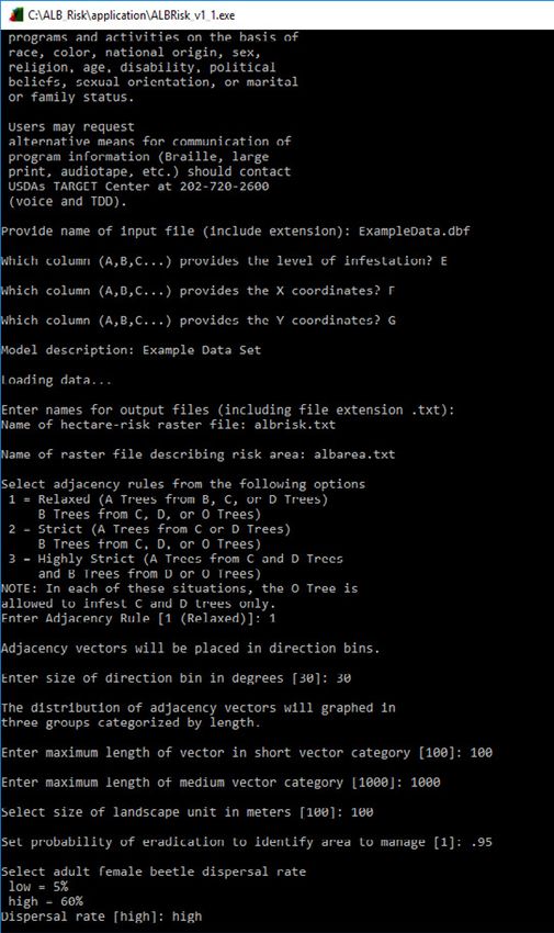
pheromones in eradication programs. Some of these
issues include a potentially short (
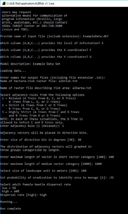
Figure 7.—Surveys based on visual searches for exit holes
and oviposition pits are the most common tool used to find
individual infested trees Mike Bohne of the USDA Forest Service,   Figure 8.—Surveys by tree climbers provide access to a larger
is shown conducting a search. USDA photo by R. Anson Eaglin.       portion of the tree canopy and provide increased confidence
                                                                   in beetle detection rates, though the process takes longer than
                                                                   ground surveys. USDA APHIS photo.

Carteret, and Linden, NJ, New York City, NY, and                   Ongoing Needs to Estimate Risk,
Boston, MA. These methods have also been effectively               Optimize Surveys, and Track
applied to larger landscapes such as those around
                                                                   Eradication Progress
Worcester, MA, and Bethel, OH, with surveys at both
locations identifying many fewer infested trees as                 Due to the cost and effort required to survey large
surveys progress. However, in large landscapes with                landscapes, it is very important to prioritize where to
dense tree cover, such as those around Worcester and               deploy survey crews in order to maximize eradication
Bethel, and in the newly detected infestation near                 efficiency and efficacy. Two additional challenges to
Hollywood, NC, survey crews are faced with the task                identifying priority areas for survey remain. First, as
of checking millions of individual host trees for signs            surveys shift from efforts to identifying the boundaries
of infestation. Also, eradication programs typically               of the infestation (delimitation), to the identification
include a multi-survey protocol that requires each tree            and removal of all infested trees (eradication), there
and stand to be surveyed multiple times. While these               is a need to identify priority areas where survey
multiple surveys greatly improve the efficacy of the               crews may have the greatest impact on eradication
programs, they also increase the number of surveys a               progress. Second, as eradication programs reduce the
program must undertake.                                            number of infested trees on the landscape, finding the
                                                                   remaining but increasingly rare infested trees becomes
                                                                   more challenging, and targeted surveys may become
                                                                   increasingly important to help programs efficiently
                                                                   estimate and mitigate remaining risk on the landscape.
                                                                   This approach may also help determine the point at
                                                                   which surveys have achieved an acceptable level of
                                                                   overall risk reduction. Risk maps and outputs produced
                                                                   by ALB Risk version 1.1 can support these efforts.

                                                                                                                                     5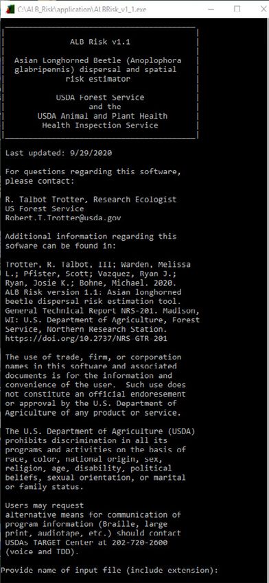
ALB RISK VERSION 1.1
ALB Risk version 1.1 (v1.1) is a computer software program that estimates the distribution
of risk within an area infested by the Asian longhorned beetle based on dispersal patterns
specific to that infested area and the locations and infestation levels of known infested trees.
The program generates risk maps, identifies priority areas for management, estimates the
statistical boundaries of the infestation, and estimates the potential return on survey effort
based on the locations of known infested trees. These steps are based on the computation
methods described in Trotter and Hull-Sanders (2015) and Trotter et al. (2018), which have
been expanded to include additional output that may be of use to eradication management
programs.

Software Summary, Structure, and Assumptions
Information on the development, conceptual structure, and assessment of the analyses used
in ALB Risk v1.1 can be found in Trotter and Hull-Sanders (2015), and Trotter et al. (2018).
This report provides an application-oriented description of the model along with a more
detailed description of how to install and run the software, how to structure input data, some
descriptions, discussions, and examples of options and model parameters included in the
software program, and an explanation of the outputs that it generates. These expanded topics
are not addressed in Trotter and Hull-Sanders (2015) and Trotter et al. (2018). Generally,
the intent of the model is to identify patterns of dispersal on the landscape based on discrete
assumptions regarding beetle dispersal behavior and use these dispersal patterns to estimate
the distribution of risk on the surrounding landscape. To accomplish this, the software uses
the input data provided by the user to carry out four tasks.

1) Reconstructing Patterns of Beetle Movement: The software analyzes infested tree records
provided by the user. The data should include a list of infested trees, their locations in X and
Y coordinates (UTM coordinates are preferred), and a categorical level of infestation for each
tree represented by values from 1 through 5. These data are used to map the infested trees and
identify connections (called adjacencies in graph theory) among the trees based on a set of
rules (adjacency rules). These rules are relatively simple and can be modified by the user. An
example set of typical rules might include:

  • The intensity of the infestation on a tree indicates the age of the infestation on the tree,
    i.e., trees with heavier infestations have been infested longer than lightly infested trees.
  • A tree is infested by a beetle that arrives from the closest tree with an older infestation.
  • A tree is infested only once but can serve as the source of infestation for multiple trees.

Using these rules, each of the infested trees on the landscape can be connected to at least one
other infested tree. By applying this process to all of the known infested trees on the landscape,
the model produces a network among the infested trees in which each connection represents a
beetle dispersal event (vector) that includes both a distance and a direction. The total number
of inferred beetle movements is therefore equal to the total number of infested trees used in
the analysis, minus one. One tree (identified by the user) is assumed to be the first infested
tree and serves as the initial source of the infestation.

2) Quantifying Dispersal Probabilities: Dispersal vectors are tabulated to produce a
probability distribution of dispersal distances, a function usually referred to as a dispersal
kernel in ecological literature. This dispersal kernel represents the probability that a beetle will
travel to a given distance. To produce dispersal kernels that include direction information, the

                                                                                                       6
dispersal vectors are grouped in direction bins (for example, all dispersal vectors that were
between 0 and 30 degrees on a compass, 30 and 60 degrees, etc.). Tabulating the vectors within
these direction bins produces direction-specific dispersal kernels. These directional dispersal
kernels estimate the probability that a beetle will disperse in a specified direction to a specified
distance.
3) Estimating Dispersal Risk on the Landscape: Placing these direction-specific dispersal
kernels around a single point produces a three-dimensional distribution of dispersal risk (an
example is shown in Fig. 27). If each infested tree is assumed to represent a center point for
this risk distribution, the three-factor dispersal kernel estimates the risk for each point on
the landscape surrounding the tree. Repeating this process for each tree and compiling the
contribution of each tree on the landscape for each location on the landscape produces a grid
of risk values in which the value for each grid point is the probability that at least one beetle
has arrived from at least one infested tree. For simplicity the software uses a landscape grid in
which sections represent 1 hectare, though the size of the landscape unit can be changed by
the user.
4) Ranking Risk on the Landscape and Optimizing Survey Sequences: The total risk for
the landscape can be described as the product of the probabilities for each hectare that the
hectare does not include an infested tree. If a hectare with risk is removed from the landscape
(i.e., the risk for the hectare has been reduced to 0) then the overall probability (product of the
remaining hectares) that any portion of the landscape is still infested is reduced. Removing
the hectares sequentially, starting with the highest risk locations, provides the most rapid
reduction in overall landscape risk. Plotting the number of hectares that have been removed
(risk reduced to 0) as a function of the overall probability of eradication provides a curve that
describes the relationship between the portion of the landscape which has been managed and
the overall probability that the beetle has been eradicated (1 – the probability that at least one
hectare on the landscape remains infested). This approach can also provide an estimate of the
total percentage of the at-risk landscape that needs to be managed to attain a specific overall
probability of eradication.
Additional Applications for Output – Informing Survey Progress: The output provided
by the software represents static estimates of risk based only on the potential dispersal of
the Asian longhorned beetle. As surveys progress, the estimated risk for each location can
be modified based on the survey results, i.e., detecting or not detecting infested trees. An
additional software tool, ALB Dynamic Risk version 1.0, can be used to produce these
dynamic risk estimates. A description of this tool and its use are provided in an upcoming
document: ALB Risk version 1.0: Tracking and Assessment Tool for Asian Longhorned Beetle
Eradications.4
4
At the time of publishing, users can obtain a beta version of ALB Dynamic Risk version 1.0 and
associated documentation by contacting Talbot Trotter at Robert.T.Trotter@usda.gov.
7ALB RISK VERSION 1.1: SOFTWARE USER GUIDE
The text uses the following fonts to identify keystrokes, files, software, data, etc.
enter = carriage return key. This may be labeled with “Enter”, “enter”, “return”, “CR”, or a
carriage return symbol depending on the computer or keyboard model or manufacturer.
Pathfiles and file names. [Calibri italic font]
Software prompts and output. [Courier New font]
Input provided by the user. [Arial black font]
Downloading, Installing, and Starting ALB Risk version 1.1
Download and install ALB Risk version 1.1 from https://doi.org/10.2737/NRS-GTR-201.
The software can be saved to any convenient location on the computer provided the user has
permission to write files to the location. ALB Risk version 1.1 (hereafter referred to as ALB
Risk v1.1) is a stand-alone program and can be run on Microsoft Windows™, or on computers
running Unix™, Linux™, or MacOS™ operating systems when combined with a Windows™
virtual machine. If the user has administrative privileges, the software can be installed by
double-clicking on the file ALBRiskv1_1_install.exe. Note that some users may need to contact
a system administrator if administrator privileges are required to add software. When the
installation launches, the following window should briefly appear (Fig. 9):
Figure 9.—Window showing the
launch of the ALBRisk v1.1 installer.
8Followed by this window (Fig. 10):
Figure 10.—Once
launched, the installer
provides information
on the version being
installed.
To continue the installation, press Next. The following window should appear (Fig. 11):
Figure 11.—The installer
will identify a default
installation location for
the software. Changing
this location may
prevent the model from
functioning correctly.
If a different location
is required by the user,
contact Robert.T.Trotter@
usda.gov to obtain a
modified version.
As shown in Figure 11, the installer will load the program and data files into a location
called C:\Program Files\..\ALB_Risk. Please note that this is NOT where the software will be
installed, rather, the files will be installed in a newly created directory C:\ALB_Risk\ for reasons
described below.5 DO NOT change the installation folder, as this may cause the software to
5
Access by users to files and directories within Program Files varies among operating systems,
administrator settings, and user profiles. Some users may not be able to add files or directories to
Program Files, or may be able to add them, but not edit or remove them. ALB Risk v1.1 both creates
and modifies files. To avoid conflicts with user access to Program Files, ALB Risk v1.1 is installed in
its own directory on the C: drive.
9generate errors or fail to run. The locations of the programs and files which allow the program
to run are hard-coded in the program, however if you need to install the programs and/or data
files in a different directory or drive, please contact Talbot Trotter (Robert.T.Trotter@usda.gov)
to request a modified version of the software. To continue the installation, select Next.
Running ALB Risk v1.1 requires the computer to have an installed version of MATLAB
Runtime™ (MathWorks, Natick, MA), which is a free set of shared libraries. At this point the
installer will check to determine whether a suitable Runtime version is already installed. If it is
not, the installer will prompt the user to install it by providing a link to the website where the
libraries can be downloaded for free. Due to this step, the installation of ALB Risk v1.1 requires
an internet connection to complete. If the computer does not have an internet connection, a
version of the installation package that includes the Runtime program is available. If MATLAB
Runtime™ is already installed on the computer, the following window should appear (Fig. 12):
Figure 12.—ALBRisk v1.1
requires the installation
of MATLAB Runtime™.
The installer will search
for MATLAB and, if one
is not installed on the
computer, will prompt
the user to download
and install a current
version.
Select Next to continue (Fig. 13):
Figure 13.—The
installer will provide
the user with
installation settings
before completing the
installation.
10Select Install, and the installation should complete, and the completed installation window
should appear (Fig. 14). Select Finish to close the window and complete the installation.
Figure 14.—When
installation is complete,
the installer will
indicate this along with
information on how to
cite the model.
To confirm the installation, open a directory explorer program (such as File Explore on
TM
a Windows™ computer) and search for a new directory called C:/ALB_Risk/. Within this
directory, there will be four subdirectories: appdata, application, sys, and uninstall. The
program itself is located within the application subdirectory and is called ALBRisk_v1_1.exe
(Fig. 15). The application subdirectory will also contain an example data set (Fig. 15) and will
be the location where output files generated by the software are saved. Double-clicking on the
ALBRisk_v1_1.exe file should launch the program. Note that when the program starts, the user
will be presented with a command window. This window may remain blank for a few minutes
the first time the software is started but should (within a minute or so) present the user with
summary text describing the version of the software. If summary information describing the
software is displayed along with the prompt:
Provide name of input file (including extension):
then the software has installed correctly. To close the program without running it, simply close
the command window using the box in the top corner.
Using the Provided Example Data as Model Input
The input data for ALB Risk v1.1 is provided by the user as a single file containing data in
which rows represent individual infested trees, and columns represent attributes describing
the trees. The dataset can include numerous attribute columns but only three are currently
used by ALB Risk v1.1. The three required columns provide the X and Y coordinates for each
tree, and an integer describing the level of infestation. A sample data set with artificial tree
records named ExampleData.dbf trees can be found in the application folder (Fig. 15). This
file can be used as a demonstration dataset and provides a template for how datasets can be
organized.
11Figure 15.—When
installed, the program
will be contained
within a folder called C:/
ALB_Risk/application,
which will contain
the program and an
example data set.
This folder is also the
location where the
program will store
output files.
ExampleData.dbf can be opened using a spreadsheet program or a geographic information
system. Note that the file can be opened using a text editor, however, the data may be shown
with unusual formatting due to the use of a .dbf file structure.
Using User-Provided Data as Model Input
The simplest way to organize and format data for ALBRisk v1.1 is to use a GIS dataset
(ArcGIS, QGIS™, CAD) in a Shapefile format. If the following conditions are met, the .dbf file
associated with the Shapefile may be used directly as the input file for the model.
1) The shapefile should be projected (or re-projected) into a Universal Transvers
Mercator (UTM) or other gridded coordinate system.
2) The attribute table should include a field (column) that provides the infestation data for
each tree. The infestation should be indicated with a single numeric integer between 1
and 5 (inclusive). Levels 1 through 4 correspond with the infestation levels A through
D used the by the Cooperative Asian Longhorned Beetle Eradication Program (A = 1,
B = 2, etc., additional information can be found at APHIS 2020). The data should also
include a single tree with an infestation category of 5 which indicates the assumed
original infested tree, which the software uses as the starting point for the infestation.
Note that it may not be necessary to know the precise location of the original infested
tree; selecting a highly infested tree from the stand where the infestation is assumed to
have started may be adequate, particularly in larger infestations.
3) The attribute table should include a column that provides the X and Y coordinates for
each infested tree. If the table does not include this data, it can be added, in ARCGIS TM
for example, this can be done using the ADDXY Function in ArcPy. ALB Risk v1.1
requires each tree to have a unique location (X-Y coordinate), however the software
will accept datasets that include multiple trees with the same coordinates. If a dataset
includes trees with matching coordinates, the locations for the matching trees will be
shifted slightly (up to a few centimeters) to provide each tree with a unique location.
The .dbf file associated with the Shapefile format can be used directly as the data input file
for ALB Risk v1.1. If the data is in a .dbf format, the data file will include headers which will
be ignored by ALB Risk v1.1. The use of specific column headers or attribute field labels are
not required. Before running ALB Risk v1.1, note which columns (first, second, ninth, etc.)
provide the X, Y, and infestation data, as the user is required to tell ALB Risk v1.1 where to
find the information in the input file. The data file should be saved to the directory C:/ALB_
Risk/application, the same directory where ExampleData.dbf is located (Fig. 15). This is the
only location from which the software will read data files.
12Analysis Settings and Options
Users are encouraged to run the software using the
provided example data (ExampleData.dbf) to become
familiar with settings, options, and data formats.
The following instructions and examples assume the
provided example data are being used, though the
process is the same when using user-provided data.
Start the software: After installing the software,
navigate to C:/ALB_Risk/application and double-
click on the file ALBRisk_v1_1.exe. This will open a
new command-prompt style window. NOTE: After
starting the program, the window that opens may
appear blank for a few moments. This delay is normal
and may be more pronounced if this is the first time
the software has been launched. Once the software
initiates, the computer screen should appear as Figure
16. Note that the window may need to be expanded or
the user may need to scroll within the window to view
the full text.
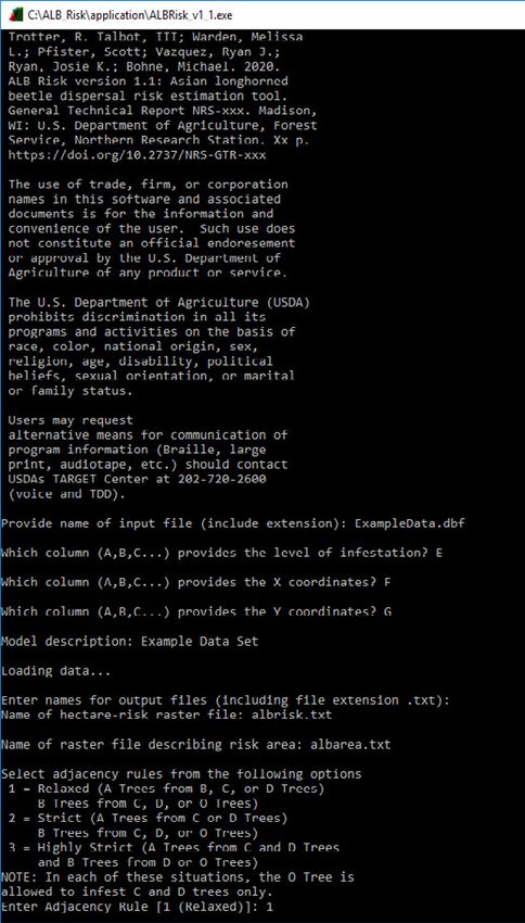
Providing input data: When the software initiates, the
window will display the software version and contact
information, and the user will be prompted to provide
the name of the file that includes the infested tree
records (Fig. 16). When running the example data,
simply type ExampleData.dbf. If a user-provided file
is being used, type the name of the file including the
suffix (i.e., .dbf). Note that the software will only be
able to process data in files stored in the same location
(i.e., folder) as the program itself, specifically, in the
directory C:/ALB_Risk/application. If it is necessary to
use files stored in a different location, please contact
Talbot Trotter (Rober.T.Trotter@usda.gov) to arrange
to receive a modified version of the software. Figure 16.—Double clicking the file ALBRisk_v1_1.exe
will launch the model program. Once launched, the
program will provide information and prompt the user
to identify an input data file. The model will accept many
data file formats, though a .dbf format is recommended.
13Once the name of the data file has been entered,
press enter on the computer keyboard. The
user will then be prompted to identify the
columns that provide the infestation levels, X
coordinates, and Y coordinates for the infested
trees. The software identifies columns based
on position (not column header or name),
and position is denoted using letters (the same
system used by Microsoft Excel ). Using this
TM
system, if the data of interest are stored in the
first column, type the letter A, if the values are
in the second column, enter B, for the seventh
column, type G, etc. The letters entered are not
case sensitive (both upper and/or lower case
are acceptable). To determine which columns
are to be used, open the .dbf file in a text editor,
a GIS, or in a spreadsheet program such as
Microsoft Excel (note however that newer
TM
versions of Excel™ can open .dbf files but cannot
save data to a .dbf format). In the case of the
example data provided in ExampleData.dbf
the infestation data is provided in column E, X
coordinates are in column F, and Y coordinates
in are column G (as shown in Fig. 17, bottom
of the screen). After entering each letter press
enter.
Next, the user will be prompted with:
Model description:
The text entered by the user will be included in Figure 17.—After identifying the data file, the user will be
the titles of figures produced by the software, so prompted to identify the columns that provide the level of
the user is encouraged to enter text that will be infestation, X coordinate, and Y coordinate for each tree. The
useful when reviewing these documents such user will also be prompted to provide a brief description for the
model run.
as the location of the infestation, or the names
of parameters used in the analyses (if the user is
running the analyses under varying conditions). There is no limit to the length of the text the
user enters, however using long strings of text may result in odd figure titles; limiting the text
to 30 characters will generally produce reasonable figures. If the user is running the Example
Data, type “Example Data Set” or some other suitable text to describe the analyses, then press
enter.
Naming output data files: At this point, the software will load the data. Depending on the
size of the data set being loaded, this may take a few moments. Once the data is loaded, the
software will indicate the data is loaded and the program is ready to continue by prompting
the user to provide names for the two output raster data sets. The two output rasters will
be identical with regards to the area analyzed and the locations of the hectares analyzed.
However, the two files provide different output. The first file will be named based on the name
provided by the user at the prompt:
Name of hectare risk raster file:
14This file provides the estimated probability of infestation for each hectare within the analyzed
area, with values ranging from 0 to 1. In the example shown in Figure 18 the file named used
is albrisk.txt. The user will then be prompted to provide a name for the second output file
with the message:
Name of raster file describing risk area:
This file provides an output raster with an extent that matches the first, however in this case,
the values for each hectare will be binary (0 or 1). Hectares with the value 1 collectively
describe the area that contains a specified overall risk (with the risk value set by the user, as
described in the section below titled “Set Probability Threshold to Identify the Perimeter
of the Eradication Area”, where more detailed information is provided. Briefly, the output
raster provides the minimum area that must be managed to achieve a given probability of
eradication (probability value set by user). In this example, the file name used is albarea.
txt. Note that when naming these files, the file name should include the suffix .txt.
Selecting Adjacency Rules: The first
parameter option allows the user to select
the set of adjacency rules the software will
use to reconstruct the movement of beetles
on the landscape. These rules determine
which trees may serve as a source of beetles.
In ALB Risk v.1.1, there are three options
available: Relaxed, Strict, and Highly Strict
(Fig. 18, bottom of screen).
Relaxed dispersal (default option 1) assumes
that any tree with exit holes can serve
as a source for dispersing beetles. Strict
dispersal (option 2) assumes that beetles
emigrate only from trees with higher levels
of infestation (specifically C and D level
trees with their corresponding 10-100 and
100+ exit holes) and comports with the
idea that beetles are unlikely to disperse
from their natal tree until the tree has been
heavily infested and damaged by the beetle.
Highly Strict (option 3) is extends the Strict
dispersal assumption by assuming only D
level trees will produce dispersing females. It
is recommended that the user select option
1 (the default), as published data suggests
this may be the most parsimonious option
(Trotter and Hull-Sanders 2015). The user
may select the option by typing the option
number (1, 2, or 3). If the user presses enter
without typing a number, the software will
default to option 1. For each of the following
user-options, pressing enter will select the
default option shown in brackets.
Figure 18.—Users can select from three different sets of
assumptions regarding beetle dispersal. Option 1 is recommended.
15Selecting Direction Bin Size: The
reconstruction of ALB dispersal patterns
on the landscape produces a collection of
dispersal vectors, each with a direction
and distance. To estimate the probability
that a given beetle will disperse to a given
distance and in a given direction, dispersal
vectors are categorized into direction bins.
The size of each bin is measured in degrees,
for example the default value used by the
software is 30 degrees (Fig. 19, bottom of
the screen) which categorizes each dispersal
event into one of 12 direction-specific bins
(corresponding to the 30 degree ranges that
correspond to north-north-east, northeast,
east-north-east, etc.). The size of the
direction bins can be modified by the user
to either refine (by using smaller values)
or generalize (by using larger values) the
direction data. However, the user is limited
to values that are factors of 360 degrees
(i.e., values of 1, 2, 3, 4, 5, 6, 8, 9, 10, 12, 15,
18, 20, 24, 30, 45, 60, 90, 120, 180, or 360
degrees). There is a tradeoff between bin
size and sample size; as the directional bins
become smaller, the estimated patterns of
dispersal become more precise, however
as the size of the bins decreases, so will
the number of dispersal vectors within the
bin. As a result, the dispersal probabilities
are based on smaller sample sizes which
makes them more subject to stochastic
influences. Conversely, if direction bins
are made larger, the sample size in each
bin will increase but at the cost of more Figure 19.—The direction of each estimated beetle movement
specific directionality. Setting the value to will be placed into a direction bin to facilitate analyses. Bin size
360 degrees will place all of the dispersal is defined using degrees. Larger bins will increase the sample
size used for each direction but will produce more generalized
vectors into a single bin producing a single, patterns. Smaller sizes increase the specificity of the model at the
nondirectional dispersal kernel. cost of sample sizes. Generally, a bin size of 30 degrees provides a
reasonable balance.
Graphing Dispersal Vectors by Size
Beetle dispersals can span a range of distances, from as short as a few centimeters to multiple
kilometers, and can occur in any direction. Landscape structures such as topography and
vegetation distribution, and physical factors such as wind direction, may influence patterns of
dispersal. To provide users with additional tools to explore the relationship between dispersal
distance and direction, the model can produce rose-histograms for dispersal vectors in three
size categories referred to simply as “short”, “medium”, and “long” (see example in Fig. 26). The
distances that define these distance categories are defined by the user and may be useful for
exploring patterns in the data. To define short, medium, and long distances, the user identifies
two values that serve as the break points between short and medium, and medium and long
16dispersal events (Fig. 20, bottom of screen).
The units are the same as those used by
the input data set; in the case of UTM
coordinates, the units will be meters. Here,
we use the term meters for convenience.
The default values provided are 100 and
1000 meters which categorizes dispersal
distances between 0 and 100 meters as
short, distances between 100 and 1000
meters as medium, and distances longer
than 1000 meters as long. These values
could, for example, be used to evaluate
the directionality of dispersal events that
occur within a stand (~100 meters), and
those that cover more than a kilometer. It
is IMPORTANT TO NOTE that the values
set by the user are ONLY used to produce
the graphic shown in Figure 26. The
values selected to not impact or alter the
reconstruction of beetle dispersal, or the
estimation of risk on the landscape.
Size of Landscape Unit (Pixel) for
Analysis
ALB Risk v1.1 provides output data in
two rasters, and the user may set the size
of the raster pixels. The default size for a
pixel in the raster is 100 which (provided
the input data X and Y coordinates are in
meters) produces 100 by 100 meter or one
hectare pixels. This parameter also sets the
spatial unit of measure for distance bins
(as described in Trotter et al. 2018) used to
calculate risk based on distance to infested
trees. The model will analyze a landscape Figure 20.— Outputs for the model include a graph showing the
that is 400 pixels east to west, and 400 directionality of dispersal based on whether the dispersal was “short”,
pixels north to south, and centered on the “medium”, or “long.” The maximum length for the short and medium
dispersal identify the lengths that separate the three categories.
mid-point of the distribution of infested
NOTE: Changing these values does not change the analyses; it is
trees. As the pixel size changes, the size of included only as a tool to explore the data using Figure 26.
the landscape analyzed will also change.
The default setting of 100 meters (Fig. 21, bottom of screen) applies the analyses to a 40 km x
40 km area. The use of the default value is recommended for users and in the following text
the term hectares and pixels are used interchangeably.
17Figure 21.—The landscape is
analyzed by breaking it into a grid
with a size set using this option.
We recommend the user select the
default value of 100 meters, which
will produce output data sets at a
1-hectare scale.
Set Probability Threshold to Identify the Perimeter of the Eradication Area
In addition to calculating the estimated probability of infestation for each hectare on the
landscape, the model can produce a map that identifies the portion of the landscape that
captures a specified, overall probability that the beetle remains on the landscape, and
conversely the probability that the beetle has been eradicated. The user sets this value at the
prompt:
Set probability of eradication to identify area to manage [1]:
In the example shown in Figure 22 (bottom of screen), the value has been set to 0.95. Based
on this value, the model will identify the smallest number of hectares that can be managed
in order to achieve a 95 percent probability that the beetle has been eradicated from the
landscape. Note that the model assumes that the risk in managed hectares is reduced to 0.
If the user sets the value to 1 (the default), the model will indicate all of the hectares on the
landscape that include any calculated risk of beetle infestation. The outer perimeter of the
18Figure 22.—The software will
produce a second raster dataset
that identifies the minimum area
that must be managed to achieve
a given probability of eradication.
This setting allows the user to set
this probability. In the example
shown, the value entered is 0.95,
so the output raster will identify
the portion of the landscape to
be managed in order to achieve
a 95 percent probability that the
beetle has been eradicated from
the landscape.
at-risk area represents the total area with calculated risk and may have utility as an estimate
for the boundaries of the infestation. Note that the output raster is spatially explicit, and the
perimeter of the area with estimated risk may not be contiguous.
Adult Female Dispersal Rate
To estimate the probability that a beetle has arrived at a specified location on the landscape
it is necessary to know two parameters: the number of adult female beetles on a tree and the
proportion of those females which disperse from their natal tree.
The number of adult female beetles on a tree is estimated by assuming that 50 percent of
the emerging beetles are female, and that the tree in each infestation category includes the
maximum number of exit holes for that category. For example, a level 3 (also called level C)
infested tree has between 10 and 100 exit holes, with an assumed maximum 100 adults, 50 of
which are female and have the potential to disperse to infest new trees.
19Figure 23.—The rate at which
female beetles emigrate from their
natal tree to infest new trees is
not well documented. However,
laboratory and field data suggest
the rate can be as low as 5 percent,
or as high as 60 percent. The user
may choose to run the model
using both parameters in order to
bracket the estimated risk.
Information on the rate of female dispersal, however, is highly limited and so this parameter
remains under study. Published studies have suggested rates of dispersal as low as 5 percent
and as high as 60 percent. To accommodate this variation, the software can be run using an
assumption of either low (5 percent) or high (60 percent) dispersal rates (Fig. 23, bottom
of screen). Using the above level-3 tree example, under a low dispersal scenario the model
assumes the tree has produced 2.5 dispersing females (50 x 0.05). Under a high dispersal
scenario, the model assumes the tree has produced 30 dispersing females (50 x 0.6). The
default value used by the model is the high dispersal rate, as this represents a “worst case
scenario” structure. However users may find it informative to run the model twice—once
under each dispersal rate—to examine how changes in dispersal rate on the landscape may
change patterns of risk.
Press enter on the keyboard to start the model. The window will indicate the software is
running and will display a message when complete as shown in Figure 24.
20Figure 24.—When the analyses
has been completed, as indicated
at the bottom of this window,
and the software will open six
additional windows with graphs
and figures.
Evaluating the Output
When ALB Risk v1.1 completes its analyses, the software will display six graphs. These graphs
provide insight into the structure of the data and patterns of beetle dispersal on the landscape.
Each graph is explained below. Note that when the command window is closed, the graphs
will be closed without being saved. To save the graphs, use the disk icon in the upper left
corner of each graph window. Icons in the window will also allow the user to zoom in and pan
over the graph.
Reconstructed Patterns of Beetle Dispersal
Using the rules (Relaxed, Strict, and Highly Strict) described previously (see Fig. 18), the
software will infer the patterns of beetle movement by creating vectors among the infested
trees. A graphical representation of these movements on the landscape (Fig. 25) is provided by
the software. Each line represents the movement of (at least) one beetle from a source tree to
a receiving tree. Note also that the text entered by the user as a description of the analyses (in
this case, “Example Data Set”) is included in the title.
21Figure 25.—The analysis of risk
on the landscape is based first on
reconstructing how the beetle
disperses. This graph shows the
estimated pattern of dispersal
within the infested area based on
the artificial data provided.
Short-, Medium-, and Long-Distance Dispersal Patterns
A rose-histogram plot showing the number of beetle dispersal events (vectors) for each
direction bin is provided in Figure 26. This figure can be modified by the user (as described
in the section Selecting Direction Bin Size) and based on whether the vector is considered a
short-, medium-, or long-distance event (categories can be modified by the user). Note that
this graphic is included to provide the user with insight into beetle dispersal behavior, but
the use of short-, medium-, and long-distance categories does not affect the calculation of
dispersal risk on the landscape (shown in Figure 28) and the output data files. In the example
shown, dispersal at short distances (less than 100 meters, perhaps within-stand dispesal?)
appear somewhat random, while medium dispersal distances (between 100 and 1000 meters)
are generally toward the northeast, and long dispersal events were almost always to the south.
Figure 26.—As mentioned in the
description of Figure 20, the user
can identify the distances that
will be categorized as “short”,
“medium”, and “long.” These plots
provide grap¬hical representations
of the directionality of the beetle
movements in each distance
category. In the example shown,
short dispersal events (top) appear
to have occurred in random
directions, while long dispersal
events (bottom) were strongly
biased toward the south-southeast.
22You can also read