An Evaluation of 3D-Printed Materials' Structural Properties Using Active Infrared Thermography and Deep Neural Networks Trained on the Numerical ...
←
→
Page content transcription
If your browser does not render page correctly, please read the page content below
materials
Article
An Evaluation of 3D-Printed Materials’ Structural Properties
Using Active Infrared Thermography and Deep Neural
Networks Trained on the Numerical Data
Barbara Szymanik

                                          Center for Electromagnetic Fields Engineering and High-Frequency Techniques, Faculty of Electrical Engineering,
                                          West Pomeranian University of Technology, Szczecin, Sikorskiego 37, 70-313 Szczecin, Poland;
                                          szymanik@zut.edu.pl

                                          Abstract: This article describes an approach to evaluating the structural properties of samples
                                          manufactured through 3D printing via active infrared thermography. The mentioned technique
                                          was used to test the PETG sample, using halogen lamps as an excitation source. First, a simplified,
                                          general numerical model of the phenomenon was prepared; then, the obtained data were used in a
                                          process of the deep neural network training. Finally, the network trained in this manner was used for
                                          the material evaluation on the basis of the original experimental data. The described methodology
                                          allows for the automated assessment of the structural state of 3D−printed materials. The usage of a
                                          generalized model is an innovative method that allows for greater product assessment flexibility.

                                          Keywords: active thermography; deep learning; numerical modeling; LSTM neural networks;
                                          3D-printed structure quality

Citation: Szymanik, B. An Evaluation      1. Introduction
of 3D-Printed Materials’ Structural       1.1. Quality Control of 3D−Printed Materials
Properties Using Active Infrared                The use of additive manufacturing (AM), otherwise known as 3D printing, is now
Thermography and Deep Neural              prevalent in many industries. Early on, printed structures were mostly used in the design
Networks Trained on the Numerical         and development of the devices’ prototypes. However, the progression of 3D printing
Data. Materials 2022, 15, 3727.
                                          techniques has led to the fact that these structures are becoming more common in final
https://doi.org/10.3390/ma15103727
                                          product production [1,2]. As a result of the wide range of materials available for AM,
Academic Editor: Satyam Panchal           printed elements are present in advanced industrial settings, including but not limited
                                          to the medical (for building blood vessels or constructing low−cost prosthetic parts), the
Received: 27 April 2022
                                          architectural and the automotive industries [3–7]. It is crucial to assess the quality of
Accepted: 18 May 2022
                                          these materials given their widespread use. The process of additive manufacturing can
Published: 23 May 2022
                                          be controlled at all stages—the preparation (examination of the quality of the feedstock
Publisher’s Note: MDPI stays neutral      material), production (control of the printing process), and evaluation of the end−product.
with regard to jurisdictional claims in   Herein, we focus on quality control in the final stage of 3D printing production [8–11].
published maps and institutional affil-         A great deal of work has been done in the previous decade to evaluate the quality of
iations.                                  materials produced via additive manufacturing, and a variety of approaches have been
                                          introduced. Non−destructive testing (NDT) procedures are one of the most important
                                          methodologies in the field of materials science [12–15]. The use of NDT technologies, in
                                          particular, allows for the identification and characterization of surface as well as internal
Copyright:    © 2022 by the author.
                                          defects of materials without the need for any physical interactions, such as cutting or
Licensee MDPI, Basel, Switzerland.
This article is an open access article
                                          modifying the substance. Along with these benefits, NDT techniques are designed to be a
distributed under the terms and
                                          cost−effective approach of system quality management. Non−destructive evaluations of
conditions of the Creative Commons        final AM products include the evaluation of dimensional correctness and surface quality,
Attribution (CC BY) license (https://     the evaluation of internal structure, and the detection of defects. The most widely used
creativecommons.org/licenses/by/          methods for evaluating the surface quality of printed items are vision [16], microscopy [17],
4.0/).

Materials 2022, 15, 3727. https://doi.org/10.3390/ma15103727                                                 https://www.mdpi.com/journal/materials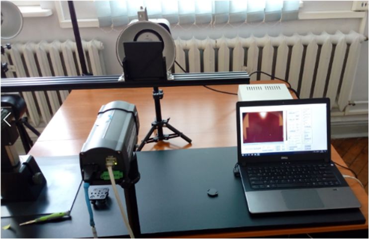
Materials 2022, 15, 3727                                                                                          2 of 22

                           and laser profilometry [18,19]. The internal structure of 3D printing, including the de-
                           tection of subsurface flaws, is mostly examined using computed tomography [20] and
                           ultrasound [21,22].
                                In this article, one of the non−destructive testing (NDT) methods—active infrared ther-
                           mography (AIT)—was utilized to examine the printed structure on a qualitative level [23,24].
                           An external energy source (here, halogen lamps) was employed to induce a thermal gra-
                           dient within the test sample in this procedure. A thermal imaging camera was used to
                           monitor the variation in temperature on the surface of the sample. Divergences (warmer or
                           colder regions) in the observed temperature distribution indicate heterogeneities within
                           the analyzed structure. The evaluated 3D−printed samples were designed in a form of a
                           basic structure—a flat cuboid with imprinted holes of varying sizes and depths, imitating
                           the object’s structural degradation.

                           1.2. Deep Neural Networks in Nondestructive Testing of Materials
                                The nondestructive testing of materials encompasses both the qualitative and quanti-
                           tative evaluation of the materials under test. It is incredibly beneficial to apply a variety
                           of machine learning methods for this assignment. A large number of machine learning
                           approaches are based on feature extraction performed by experts [25,26]. As a result, the
                           quality of the features (of the stated phenomenon or qualities) stored in the database has
                           a significant impact on the efficacy of classification or clustering algorithms, making the
                           extraction process crucial. To meet this challenge, the recent rapid growth of complex
                           multi−layered artificial neural networks (ANNs) can be observed. In general, artificial
                           neural networks (ANNs) attempt to mimic the human learning process in order to inde-
                           pendently learn features [27,28]. As a result, there is no requirement for feature extraction
                           based on human judgment in these methods.
                                In this article, to examine the state of the material, an automated defects detection
                           technique based on neural network models was developed [29–31]. An investigation of the
                           signals received during an AIT examination in the form of time–temperature characteristics
                           is carried out in this study. Consequently, the primary purpose of this study is data
                           categorization on the basis of one−dimensional sequences. The manual analysis of such
                           sequences may be difficult due to an overwhelming quantity of data, making it difficult to
                           identify patterns. Thus, the challenge of identifying patterns in time sequences in order
                           to forecast the predicted output may be accomplished via the use of artificial intelligence
                           systems. Recurrent neural networks (RNNs), as well as their modifications, are one of the
                           most successful technologies accessible in this situation [32,33].
                                As is generally known, a recurrent neural network is a kind of neural network that
                           is optimized for processing time−dependent data sequences. RNNs are often preferred
                           over other types of neural networks for applications that require sequential inputs, such
                           as voice and language recognition. RNNs are referred to as recurrent neural networks
                           because they complete the same job for each element in a sequence, with the output
                           being dependent on the results of the previous computations in the sequence. Gradient
                           calculation in RNNs is accomplished by executing a forward propagation pass followed
                           by a backward propagation pass. Back−propagation through time (BPTT) is the method
                           used here. Because the parameters are shared by all time steps in the network, the gradient
                           at each output is determined by both the current and prior time steps’ computations.
                           Although the RNN is a simple and strong model in theory, it is difficult to train well in
                           reality [34,35]. The vanishing gradient and exploding gradient difficulties are two of the
                           key reasons why this model is so problematic [36,37]. When utilizing BPTT for training,
                           gradients must pass from the last cell to the first cell. The product of these gradients
                           might either be 0 or exponentially grow. The issue of exploding gradients refers to the
                           substantial growth in the gradient’s norm during training. When long−term components
                           travel exponentially quickly to norm 0, the vanishing gradients issue occurs, making it
                           hard for the model to learn connection between temporally distant events. Whereas the
                           exploding gradient problem may be resolved relatively quickly utilizing techniques such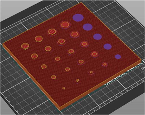
Materials 2022, 15, 3727 3 of 22
as gradient clipping, the vanishing gradient issue remains a significant concern when
employing an RNN. However, by using special modifications of recurrent networks such
as long short−term memory (LSTM), gated recurrent units (GRUs), and residual networks
(ResNets), this limitation may be solved [38,39]. Considering the above, it was determined
in this article to employ LSTM networks to process the data sequences received from
thermal imaging of 3D−printed samples.
1.3. Novelty and Significance of the Research
A key problem that occurs when utilizing neural networks to analyze diverse types
of data is the training set selection. Extracting such a collection from the same data set,
which is then assessed by a trained network, is the most often employed approach. In our
previous work, we have shown that, for this purpose, the convolutional neural networks
may be used [40], and other researchers have worked on a similar problem [41]. This
results in the obvious issue of a network adjusting to a single−use case, rendering it very
inflexible and unsuited for jobs requiring some automation. This issue may be resolved
by the use of numerical modeling. If the numerical model generated accurately represents
the true behavior of the system, we may be certain that the network trained on such
prepared numerical data will be capable of evaluating real, experimental data. The most
often utilized approach is to model the complete tested system, which, once again, may
result in an overly adapted network to the tested system. We have tested this approach
in our previous work, proving its effectivity [42]. However, we suggest a more general
approach in this work: the development of a collection of models, each of which represents
a small piece of the tested sample, containing one structural flaw and a chosen section
of the surrounding region. We shall demonstrate that such a solution enables effective
assessment of the material under test and improves the flexibility of the resulting network.
1.4. Organization of the Paper
The paper is structured as follows: the introduction discusses the non−destructive
testing of AM materials and the artificial intelligence methods used to evaluate them, with
a special emphasis on LSTM neural networks. The materials under investigation, as well
as the experimental method employed—activated infrared thermography—are discussed
in Section 2. As part of Section 3, the assumptions and structure of a parametric set of
generalized numerical models are discussed along with the numerical model optimization,
as well as the presentation of numerical findings and comparisons of numerical and
experimental results. Section 4 discusses data processing techniques and the construction of
a training data set for the neural network. The architecture of the suggested neural network
and the results of the evaluation are presented in Section 5. The paper is summarized and
concluded in Section 6.
2. Materials and Methods
The primary objective of this study was to create a method for analyzing real sam-
ples using neural networks trained on numerical data. The samples were initially tested
experimentally. In this chapter, the utilized laboratory setup, test samples, and experimen-
tal methodologies will be described. In the subsequent sections of the study, it will be
demonstrated how the tested system was reconstructed in a simplified numerical model.
Experimental Techniques and Test Samples
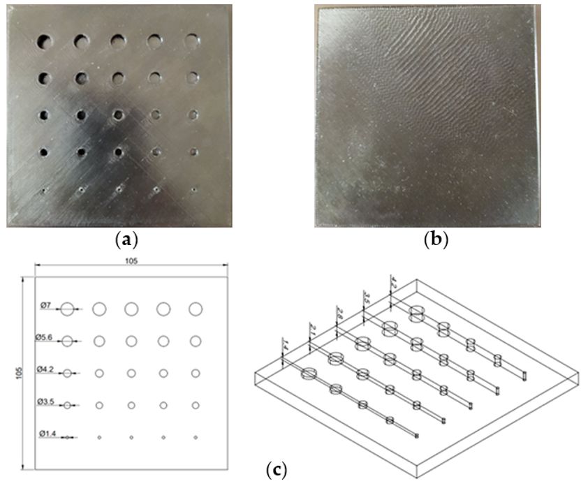
Two test samples were created using the Filament Fuse Fabrication (FFF) method,
which is one of the most widely used 3D printing technologies currently available. We
chose the broadly used polyethylene terephthalate glycol (PET−G) filament, which is
known for being both durable and simple to print with. For the sample S1, the infill
was adjusted to a maximum—100%—and for the sample S2, it was set to 30% with a
rectangular infill pattern. Both samples were designed and printed as flat plates with
dimensions of 105 × 105 × 7 mm, with a series of holes of sizes ranging from 1.4 to 7 mm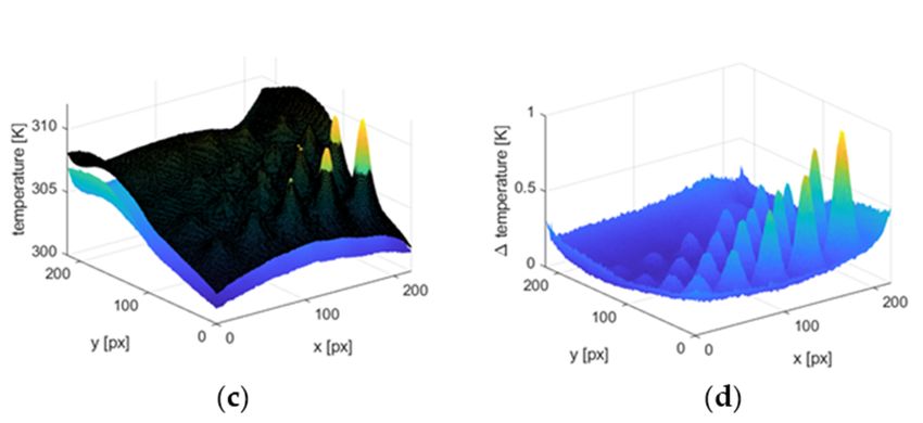
Twotest
Two testsamples
sampleswerewerecreated
createdusing
usingthe theFilament
FilamentFuse FuseFabrication
Fabrication(FFF) (FFF)method,
method,
whichisisone
which oneof ofthe
themost
mostwidely
widelyusedused3D 3Dprinting
printingtechnologies
technologiescurrently
currentlyavailable.
available.We We
chose the
chose the broadly
broadly used
used polyethylene
polyethylene terephthalate
terephthalate glycol glycol (PET−G)
(PET−G) filament,
filament, which
which isis
knownfor
known forbeing
beingboth
bothdurable
durableand andsimple
simpleto toprint
printwith.with.For Forthethesample
sampleS1, S1,thetheinfill
infillwas
was
Materials 2022, 15, 3727 adjusted to a maximum—100%—and for the sample S2, it
adjusted to a maximum—100%—and for the sample S2, it was set to 30% with a rectan- was set to 30% with a rectan-
4 of 22
gularinfill
gular infillpattern.
pattern.Both
Bothsamples
sampleswere weredesigned
designedand andprinted
printedas asflat
flatplates
plateswithwithdimen-
dimen-
sionsof
sions of105
105××105105××77mm,mm,withwithaaseries
seriesofofholes
holesof ofsizes
sizesranging
rangingfromfrom1.4 1.4to to77mm
mmand and
and depths ranging from 1.4 to 4.2 mm. An example CAD model and a photographthe
depths
depths ranging
ranging from
from 1.4
1.4 to
to 4.2
4.2 mm.
mm. An
An example
example CAD
CAD model
model and
and aa photograph
photograph of
of the
of
sample
sample
the sampleareare
are depicted
depicted inFigure
in
depicted Figure
in 1.1.Moreover,
Figure Moreover,
1. Moreover, Figure
Figure
Figure 22presents
2presents
presentsthe the inner
theinner structure
innerstructure
structureof ofthe
of the
the
printedsamples.
printed
printed samples.The
samples. Thechosen
The chosenlayer
chosen layerof ofprint
printisisvisualized
visualizedhere hereas asananoutput
outputfromfromaaaG
from G−code
G−code
−code
generatingprogram—PrusaSlicer.
generating
generating program—PrusaSlicer.The
program—PrusaSlicer. Theprinting
The printingpattern
printing patternis
pattern isvisible—rectangular
is visible—rectangularfor
visible—rectangular forboth
for bothof
both of
of
thesamples—as
the
the samples—aswell
samples—as wellas
well asthe
as thedifference
the differencein
difference inthe
in theinfill
the infillpercentage
infill percentageand
percentage andthe
and theincreased
the increasedinfill
increased infillin
infill in
in
thearea
the
the areaof
area ofthe
of thedefects
the defectsfor
defects forthe
for thesample
the sampleS2,
sample S2,which
S2, whichis
which iscrucial
is crucialfor
crucial forthe
for theresults
the resultsof
results ofthermographic
of thermographic
thermographic
inspection.This
inspection.
inspection. Thisissue
This issuewill
issue willbe
will bediscussed
be discussedin
discussed indetail
in detailin
detail infurther
in furthersections.
further sections.
sections.
Figure1.
Figure
Figure 1.Experimental
1. Experimentalsamples—(a)
Experimental samples—(a)rear
samples—(a) rear(heated)
rear (heated)and
(heated) and(b)
and (b)front
(b) front(observed)
front (observed)side.
(observed) side.(c)
side. (c)CAD
(c) CADmodel
CAD modelof
model of
of
printed
printed structures
structures (dimensions
(dimensions in
in [mm]).
[mm]).
printed structures (dimensions in [mm]).
(a)
(a) (b)
(b)
Figure2.
Figure
Figure 2.Visualization
2. Visualization of
Visualizationof the
ofthe printing
theprinting process
process
printing for
for
process chosen
chosen
for chosen layer
layer (screenshot
(screenshot
layer from
from
(screenshot thethe
the
from PrusaSlicer).
PrusaSlicer). (a)
(a)
PrusaSlicer).
sampleS1
sample S1with
with100%
100%infill,
infill,(b)
(b)sample
sampleS2S2with
with30%
30%infill.
infill.
(a) sample S1 with 100% infill, (b) sample S2 with 30% infill.
The material was examined using active infrared thermography (AIT), which used
a halogen lamp as an excitation source. The transmission technique was utilized in this
experiment: the material was heated from the back side while being monitored from the
front. Because of the poor thermal conductivity of the material under test, a long step
heating procedure was used. It was decided that the sample would be heated for 60 s and
then naturally cooled for 300 s. During this time, a thermal imaging camera was used to
record the temperature distribution on the front side of the sample at a rate of one frame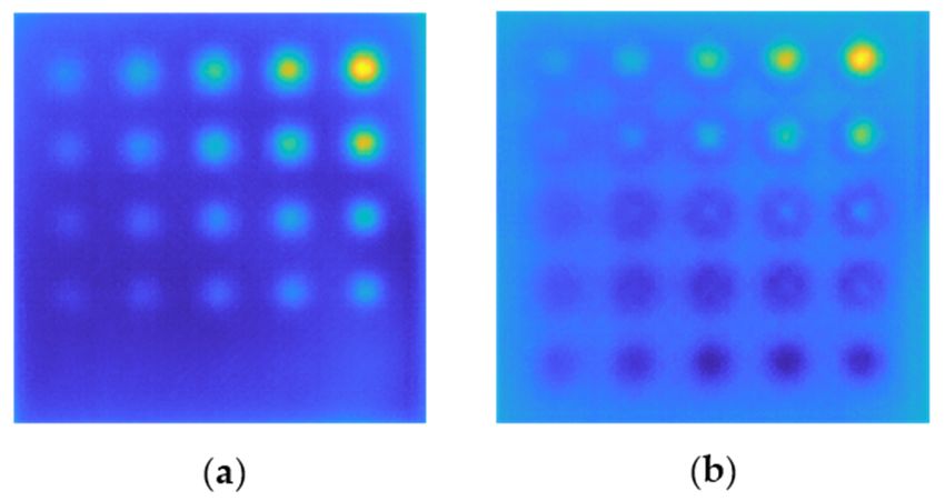
halogen
Thelamp as an
material excitation
was examined source.
usingThe transmission
active technique was(AIT),
infrared thermography utilized in this
which usedex-a
periment: the material was heated from the back side while being monitored
halogen lamp as an excitation source. The transmission technique was utilized in this ex- from the
front. Because
periment: of the poor
the material wasthermal conductivity
heated from the backofsidethe while
material under
being test, a long
monitored fromstepthe
heating procedure
front. Because waspoor
of the used.thermal
It was decided that the
conductivity of sample wouldunder
the material be heated
test, for 60 s step
a long and
Materials 2022, 15, 3727 then naturally
heating cooled
procedure wasfor 300 It
used. s. was
During this time,
decided a thermal
that the sample imaging
would becamera
heatedwasfor 60used
5sofandto
22
record the temperature distribution on the front side of the sample at a rate
then naturally cooled for 300 s. During this time, a thermal imaging camera was used to of one frame
per second.
record As a result ofdistribution
the temperature this experiment,
on the360 thermograms,
front ready for
side of the sample at further
a rate ofprocessing,
one frame
were
per produced.
persecond.
second.As The experimental
Asaaresult
resultof
ofthis setup
thisexperiment, is
experiment,360 illustrated in
360thermograms, Figure
thermograms,ready 3.
readyfor
forfurther
furtherprocessing,
processing,
wereproduced.
were produced.The
Theexperimental
experimentalsetup
setupisisillustrated
illustratedininFigure
Figure3.3.
Figure 3. Photo of the experimental setup.
Figure 3. Photo of the experimental setup.
Figure 3. Photo of
3. Numerical the experimental setup.
Model
The numerical
3.3.Numerical
Numerical Model model for this study was created using the commercial soft-
Model
ware−Comsol Multiphysics.
Thenumerical
numerical model The calculations
forstudy
this study werecreated
was performed utilizing
using Finite Element
the software
commercial soft-
The model for this was created using the commercial −Comsol
Method (FEM),
ware−Comsol with Comsol
Multiphysics. modules
The developed
calculations to
were evaluate
performedheat transfer
utilizing via conduction
Finite Element
Multiphysics. The calculations were performed utilizing Finite Element Method (FEM),
and radiation
Method (FEM),phenomena.
with developed
Comsol modules developed to evaluate heat transfer
with Comsol modules to evaluate heat transfer via conduction andvia conduction
radiation phe-
and radiation phenomena.
nomena.
3.1. General Description of the Model
3.1.
3.1.General
FigureDescription
General 4 depicts the
Description ofofthe Model
geometry
the Model of the numerical model created in Comsol. The heat
source (in
Figure this
4 experiment,
depicts the
Figure 4 depicts the geometry a halogen
geometry ofoflamp)
the was replicated
thenumerical
numerical modelusing
model created a hollow
created ininComsol.conical
Comsol. Thealumi-
The heat
heat
num
source tube
(in with
this a point
experiment, heat
a source
halogen placed
lamp) within
was at a
replicated 15 cm
using a distance
hollow
source (in this experiment, a halogen lamp) was replicated using a hollow conical alumi- from
conical the sample.
aluminum
Figure
tube
numwith 4badepicts
tube pointaheat
with the
pointsource’s
source location.
heatplaced
source withinIn at
placed order
a 15to
within cmmake
a 15the
cmmodel
atdistance from more
the
distance general,
sample.
from it was
Figure
the 4b
sample.
decided
depicts to
the simulate
source’s only
location. theInsample
order with
to makea 100%
the print
model density.
more As
general,
Figure 4b depicts the source’s location. In order to make the model more general, it was wasit the
was case in
decided the
to
experiment,
simulate only thethetemperature
sample with isa measured
100% print on the
density.samples’
As was front
the surface
case
decided to simulate only the sample with a 100% print density. As was the case in the in while
the the rear
experiment, sur-
the
face is heated.
temperature
experiment, isthe
measured
temperature on the samples’ front
is measured on the surface while
samples’ thesurface
front rear surface
whileistheheated.
rear sur-
face is heated.
Figure4.
Figure 4. Numerical
Numericalmodel
modelgeometry.
geometry.(a)(a)
The view
The on the
view on single−defect sample
the single−defect with the
sample heat
with thesource,
heat
(b) detail
source, (b)of the modeled
detail of the halogen
modeled lamp—heat
halogen reflecting,
lamp—heat hollowhollow
reflecting, cone with
conepoint
with heat source
point heat placed
source
Figure 4. Numerical model geometry. (a) The view on the single−defect sample with the heat source,
inside.inside.
placed
(b) detail of the modeled halogen lamp—heat reflecting, hollow cone with point heat source placed
inside.
Our primary objective was to develop an effective, simplified model that does not
completely replicate the whole original sample, but rather a subset of it. The utilization
of numerical data obtained in this manner for network training enables the examination
of samples with a variety of geometries and nearly any pattern of defects. Thus, the
numerical model comprises a single defect located in the center of a small region. The
model was suitably parameterized in order to collect data correlated with defects of various
diameters and depths, as well as those positioned at varied distances from the heat source.
The diameter of the defect changes between 1 mm and 8 mm (19 steps), the depth varies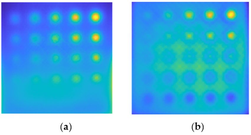
completely replicate the whole original sample, but rather a subset of it. The utilization of
numerical data obtained in this manner for network training enables the examination of
samples with a variety of geometries and nearly any pattern of defects. Thus, the numer-
ical model comprises a single defect located in the center of a small region. The model was
Materials 2022, 15, 3727 suitably parameterized in order to collect data correlated with defects of various diame- 6 of 22
ters and depths, as well as those positioned at varied distances from the heat source. The
diameter of the defect changes between 1 mm and 8 mm (19 steps), the depth varies be-
tween 1 mm and 6 mm (15 steps), and the heat source is fixed in three positions: centered
between 1 mm and 6 mm (15 steps), and the heat source is fixed in three positions: centered
on
on the
the defect,
defect, on
on the
the corner
corner of
of the
the modeled
modeled area
area plates,
plates, and
and beyond
beyond the
the plate
plate at
at aa distance
distance
of half its diagonal. We obtained a total of 855 distinct models. Figure 5 illustrates
of half its diagonal. We obtained a total of 855 distinct models. Figure 5 illustrates the the
parametrization procedure.
parametrization procedure.
Figure 5. The
Figure 5. The parameterization
parameterization of the numerical
of the numerical model.
model. (a) Chosen defects
(a) Chosen defects diameters,
diameters, (b)
(b) chosen
chosen
defects’ depths, and (c) positions of the center of the heating source.
defects’ depths, and (c) positions of the center of the heating source.
Calculations wereperformed
Calculations were performedusing
usingthe
theHeat
HeatTransfer
Transfer with
with Surface
Surface to Surface
to Surface Radia-
Radiation
tion module,
module, which which
usesuses the radiosity
the radiosity method
method to represent
to represent radiation
radiation on diffuse
on diffuse surfaces.
surfaces. In
In
thisthis case,
case, wewe suppose
suppose that
that the
the onlysource
only sourceofofheat
heatininthe
thesystem
systemisisradiation
radiation [43,44].
[43,44]. In
In
general, the following partial differential equation is used to solve the time−dependent
general, the following partial differential equation is used to solve the time−dependent
heat
heat transfer in solids
transfer in solids problem:
problem:
∂T + ∇( + ) = (1)
ρC p + ∇(q + qr ) = Q (1)
where ∂t
denotes the diffuse reflectivity, G is the irradiation, is the surface emissivity,
and ρ( d )denotes
where is the power radiated
the diffuse acrossGallis wavelengths,
reflectivity, the irradiation,according to theemissivity,
e is the surface Stefan–Boltz-
and
mann
eb ( T ) islaw.
the The
powermost criticalacross
radiated aspectallhere is the heataccording
wavelengths, flux introduced at the heated surface
to the Stefan–Boltzmann law.
via radiation
The ( ).aspect
most critical The following
here is theformula
heat fluxis introduced
dependent at onthe
twoheated
significant
surface variables: total
via radiation
irradiation
(q and radiosity.
r ). The following formulaThe term “irradiation”
is dependent refers to variables:
on two significant the entire total
incoming radiative
irradiation and
flux induced
radiosity. Theby external
term energy sources,
“irradiation” refers towhereas
the entire “radiosity”
incomingrefers to the
radiative fluxsum of diffu-
induced by
sively
external reflected
energy and emitted
sources, radiation:
whereas “radiosity” refers to the sum of diffusively reflected and
emitted radiation:
= + ( ) (2)
J = ρ G + ee ( T ) (2)
where denotes the diffuse reflectivity,dG is theb irradiation, is the surface emissivity,
where
and ρ( d )denotes the diffuse
is the power radiated acrossGallis wavelengths,
reflectivity, the irradiation,according
e is the surface
to theemissivity, and
Stefan–Boltz-
eb ( T ) is
mann theRadiative
law. power radiated across
heat flow canall
thuswavelengths,
be defined according to the Stefan–Boltzmann
as the difference between incident and law.
Radiative heat flow can thus be defined as the
emitted radiation (radiosity and specular reflected radiation): difference between incident and emitted
radiation (radiosity and specular reflected radiation):
= −( + ), (3)
where is the specular reflectivity.qrAssuming = G − (J + theρsmaterial
G ), behaves as an ideal grey body (3)
(as most opaque substances do), we finally obtain the correct formula for the radiative
where
boundary ρs iscondition
the specular reflectivity.
by utilizing theAssuming
radiative the material
inward heat behaves as an
flux, ready toideal grey body
be included in
(as most (1):
Formula opaque substances do), we finally obtain the correct formula for the radiative
boundary condition by utilizing the radiative inward heat flux, ready to be included in
Formula (1):
qr = e( G − eb ( T )) (4)
Notably, the halogen lamp housing (see Figure 4), which is modeled as a conical,
hollow object, is here regarded as a diffuse mirror, which is defined as a surface with
zero emissivity. Diffuse mirror surfaces are frequently used as approximations for a
well−insulated surface on one side, and for which convection effects on the opposite
(radiating) side can be neglected. It is similar to a mirror in that it absorbs all incident
Materials 2022, 15, 3727                                                                                                  7 of 22

                           radiation and then reradiates it in all directions. On a diffuse mirror boundary, the radiative
                           heat flux is equal to zero.

                           3.2. Optimization Approach for Material Parameters Estimation
                                 A critical component of this work is the correspondence between the numerical and
                           experimental results. Naturally, as intended, the model used to train the network differs
                           significantly from the real laboratory setup. Nonetheless, our objective is to obtain a strong
                           correlation between the experiment and the model, as well as the maximum possible
                           consistency of the results within the defects. Due to the fact that the numerical model
                           employed a sample with a print density of 100%, the optimization procedure took into
                           consideration only the experimental results obtained for sample S1 (100% print). The actual
                           physical parameters of the sample may change slightly from the parameters reported in the
                           literature for the PET−G material. Additionally, the modeled heat source is much different
                           from the actual lamp. As a result, the heating power, which was adjusted to 1000 W during
                           the experiment, should be treated as an unknown variable in the model. As we have
                           observed, little variations in the aforementioned parameters result in significant variances
                           in the time–temperature characteristics acquired for the numerical results. As a result, we
                           propose employing the optimization method to accurately predict the model’s selected
                           physical parameters [45–47].
                                 Optimization was carried out in a hybrid Matlab/Comsol system. In Matlab, the
                           optimization toolbox was employed. The optimization approach utilized a well−known
                           pattern search (PS), which is a subgroup of direct search methods. Direct search is an
                           optimization technique that does not require knowledge of the objective function’s gradient.
                           The mentioned algorithms examine a group of points around the current position, looking
                           for one where the objective function value is lower than the current point.
                                 In this study, the optimization parameters, normalized to [0,1], are: source power P (in
                           the range 900–1500 (W)), specific heat capacity Cp (in the range 900–1500 (J/(kg·K))), density
                           ρ (in the range 900–1500 (kg/m3 )), and thermal conductivity k (from 0.1 to 0.5 (W/(m·K))).
                           It should be highlighted that because the model shows a single defect at a time rather than
                           a pattern of defects (like the actual sample does), the primary issue that has been neglected
                           here is the effect of other defects on the background temperature distribution. We will
                           demonstrate that, despite this significant simplification, our approach allows for effective
                           network training on the numerical model. However, it is evident that we will not attain
                           complete consistency between the numerical model’s background and the real sample’s
                           background. As a result, this task is omitted in this optimization, and we instead focus on
                           adjusting the time–temperature characteristics of the flaws. Figure 6 shows several points of
                           interest. Region P1 contains a defect that is 1.4 mm deep and 7 mm in diameter, and area P2
                           contains a defect that is 4.2 mm deep and 7 mm in diameter. A comparable area was chosen
                           based on numerical data (see Figure 6b), denoted by P. The minimized objective function
                           calculates the sum of mean square errors (MSE) between the averaged time–temperature
                           characteristics from selected areas of the experimental and numerical results:
                                                360                                      360
                                             ∑ t =1                                   + ∑t=1 DP2 exp (t) − DP2num (t) ,
                                                                                 2                                  2
                               Objective =            DP1 exp (t) − DP1num (t)                                               (5)

                           where t denotes time, and DPexp (t), DPnum (t) are averaged time–temperature characteristics
                           from chosen regions for experimental and numerical data, respectively.
                                The starting point was chosen arbitrarily. At each optimization iteration, Comsol was
                           used to calculate the number of models for the defect with a set depth and diameter while
                           varying the optimization parameters mentioned previously. Each generated model was
                           used to extract data from the P area. After averaging the data, they were compared to the
                           relevant experimental data using the aforementioned objective function. Figure 7 depicts
                           the algorithm diagram.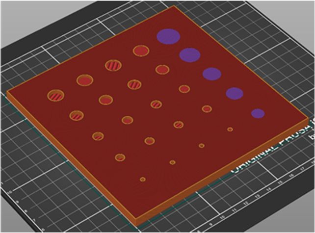
x FOR PEER REVIEW
Materials 2022, 15, 3727 8 of 22
23
Figure 6. Localization of the areas taken under account in the optimization process. (a) Areas P1 and
P2 localized on the chosen experimentally obtained thermogram, (b) area P localized on numerical
thermogram.
The starting point was chosen arbitrarily. At each optimization iteration, Comsol was
used to calculate the number of models for the defect with a set depth and diameter while
varying the optimization parameters mentioned previously. Each generated model was
used to extract data from the P area. After averaging the data, they were compared to the
relevant Localizationofdata
6.experimental
Figure 6. Localization of
thethe areas
areas
using taken
taken
the under
under account
account
aforementioned inoptimization
in the the optimization
objective process.
process.
function. 7 (a)
(a) Areas
Figure Areas
P1 and
depicts
P2
P1 localized
and P2 on the
localized
the algorithm diagram.chosen
on the experimentally
chosen obtained
experimentally thermogram,
obtained (b) area
thermogram, P localized
(b) area P on numerical
localized on
thermogram.
numerical thermogram.
The starting point was chosen arbitrarily. At each optimization iteration, Comsol was
used to calculate the number of models for the defect with a set depth and diameter while
varying the optimization parameters mentioned previously. Each generated model was
used to extract data from the P area. After averaging the data, they were compared to the
relevant experimental data using the aforementioned objective function. Figure 7 depicts
the algorithm diagram.
Figure
Figure7.7.The
Thechart
chartflow
flowofofthe
theoptimization
optimizationalgorithm.
algorithm.
Table11compares
Table comparesthe
theparameters
parametersspecified
specifiedininthe
theliterature
literaturefor
forPETG
PETGmaterial
materialtotothose
those
determinedduring
determined duringthe
theoptimization
optimizationmethod.
method.As Ascancanbebeseen,
seen,the
themost
mostsignificant
significantchange
change
concernsthe
concerns thesource’s
source’spower,
power,which,
which,asaspreviously
previouslysaid,
said,should
shouldbebetreated
treatedasasananunknown.
unknown.
Table 1. Comparison between the important parameters before and after the optimization process.
Figure The chart flow ofHeat
Power7.[W]
Capacity
the optimization algorithm. Density Thermal Conductivity
Cp [J/(kq·K)] ρ [kg/m3 ] k [W/(m·K)]
Literature data 1 Table 1 compares the parameters
1000 1242 specified in the literature for PETG material
1200 0.225 to those
Optimized values 1363 1110 1339 0.222 change
determined during the optimization method. As can be seen, the most significant
concerns
1 the
From PET− source’sData
G Technical power, which, as previously said, should be treated as an unknown.
Sheet—Fiberlogy.
To illustrate the optimization findings, the temperature–time characteristics of the
numerical and experimental results were compared. The results from the P1, P2, and P
regions were averaged for this purpose. Figure 8 depicts the outcome. As can be observed,
the shape of the numerically produced curves is well−correlated with the experimental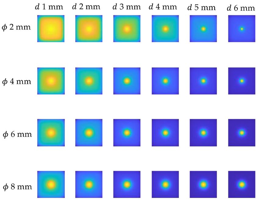
. From PET−G Technical Data Sheet—Fiberlogy.
1
To illustrate the optimization findings, the temperature–time characteristics of the
numerical and experimental results were compared. The results from the P1, P2, and P
Materials 2022, 15, 3727 regions were averaged for this purpose. Figure 8 depicts the outcome. As can be observed, 9 of 22
the shape of the numerically produced curves is well−correlated with the experimental
results, even prior to optimization, demonstrating the model’s sound physical assump-
tions. On
results, theprior
even othertohand, an improved
optimization, quantitative
demonstrating theagreement was physical
model’s sound also obtained follow-
assumptions.
ing optimization. The largest difference between the numerical and experimental
On the other hand, an improved quantitative agreement was also obtained following results
for the P1 area was 1.86 K, which is slightly more than 10% of the reference value,
optimization. The largest difference between the numerical and experimental results for whereas
the P1
the maximum
area wasdifference for is
1.86 K, which theslightly
P2 area wasthan
more 1.3410%
K, which
of the is about 8%
reference of the
value, reference
whereas the
value.
maximum difference for the P2 area was 1.34 K, which is about 8% of the reference value.
Figure 8.8.Averaged
Figure Averagedtime–temperature
time–temperaturecharacteristics
characteristics from
from regions
regions P1 and
P1 and P2 compared
P2 compared withwith nu-
numeri-
merical
cal data. data. (a) Comparison
(a) Comparison of the experimental
of the experimental (blue
(blue line) line) characteristic
characteristic for the
for the region region
P1 and P1 and
numerical
numerical
result: result:
yellow yellow line—before
line—before optimization,
optimization, red (b)
red line—after. line—after. (b)comparison
Analogical Analogical for
comparison
region P2.for
region P2.
3.3. The Comparison between Experimental and Numerical Results
3.3. The Comparison
Figure between
9 illustrates Experimental
the results and Numerical
of an inspection of realResults
samples using the active thermog-
raphyFigure
method.9 illustrates the resultspresented
The thermograms of an inspection of real samples
are unprocessed usingthe
and depict thetemperature
active ther-
mography method.
distribution The thermograms
on the surface of the tested presented
samples areafterunprocessed andthe
60 s, i.e., after depict the process
heating temper-
ature
is distribution
complete. Figureon 9a the surface
depicts of the tested
a thermogram forsamples after(100%
the S1 plate 60 s, i.e., after
infill), andthe heating
Figure 9b
process is
presents complete. Figure
a thermogram for the9aS2depicts
samplea(withthermogram forAs
30% infill). thecanS1be
plate
seen,(100%
these infill),
results and
are
Figuredissimilar.
rather 9b presentsWhereas
a thermogram
defectsforarethe S2 sample
evident (with
as hot spots30%in infill).
sampleAsS1, can be seen,
smaller these
defects
results are
(starting rather
with dissimilar.
those Whereas defects
with a diameter are evident
of 4.2 mm) as hot spots
are apparent in sample
as cooler spots S1, smaller
in sample
S2. It relates
defects to the
(starting printing
with those process itself−forofitems
with a diameter with are
4.2 mm) a lower printas
apparent density:
cooler internal
spots in
structural
sample S2.features (such
It relates as holes)
to the printingareprocess
produced with the
itself−for itemssupport
with ainlower
the formprintofdensity:
a layer
with a 100%
internal print density.
structural featuresThese
(suchsupports
as holes) areare readily
produced evident
with inthethe cross−in
support section shown
the form of a
in Figure
layer with2.aDue100%to print
the fact that these
density. These reinforced
supportsareas of the printout
are readily evident in provide a stronger
the cross−section
Materials 2022, 15, x FOR PEER REVIEW 10 of 23
barrier
shown to in heat than
Figure 2. their
Due surroundings
to the fact thatwith only
these 30% infill,
reinforced the thermal
areas signatures
of the printout of
provide thea
flaws are visible as cooler areas.
stronger barrier to heat than their surroundings with only 30% infill, the thermal signa-
tures of the flaws are visible as cooler areas.
Figure9.9.Exemplary
Figure Exemplaryexperimental
experimental results
results forfor sample
sample S1and
S1 (a) (a) and S2 The
S2 (b). (b).thermograms
The thermograms are ob-
are obtained
tained after the heating process—60 s of the observation.
after the heating process—60 s of the observation.
Aspreviously
As previously stated,
stated, optimization
optimization was
was performed
performed on on aa sample
sample with
with aa 100%
100% infill,
infill,
implyingthat
implying thatthe
thenumerical
numericalmodel’s
model’s results
results should
should be be comparable
comparable to those
to those obtained
obtained ex-
exper-
perimentally
imentally for sample.
for this this sample.
FigureFigure 10 illustrates
10 illustrates the results
the results for a variety
for a variety of defects’
of defects’ di-
diameters
ameters and depths. As can be noticed, the flaw is visible in all the images as a warmer
area. The qualitative difference between the experimental and numerical results is the dis-
tribution of the background temperature—it is notably more homogenous in the numeri-
cal data. As previously stated, this is a presumed effect due to the fact that the influence
Figure 9. Exemplary experimental results for sample S1 (a) and S2 (b). The thermograms are ob-
                           tained after the heating process—60 s of the observation.

Materials 2022, 15, 3727         As previously stated, optimization was performed on a sample with a 100%10infill,             of 22
                           implying that the numerical model’s results should be comparable to those obtained ex-
                           perimentally for this sample. Figure 10 illustrates the results for a variety of defects’ di-
                           ameters and depths. As can be noticed, the flaw is visible in all the images as a warmer
                           and depths. As can be noticed, the flaw is visible in all the images as a warmer area. The
                           area. The qualitative
                           qualitative  differencedifference
                                                     between thebetween    the experimental
                                                                    experimental              and numerical
                                                                                    and numerical     results isresults is the dis-
                                                                                                                 the distribution
                           tribution  of  the background    temperature—it      is notably  more  homogenous
                           of the background temperature—it is notably more homogenous in the numerical           in the  numeri-
                                                                                                                              data.
                           cal data. As    previously  stated, this  is a presumed    effect due  to the fact that  the
                           As previously stated, this is a presumed effect due to the fact that the influence of other  influence
                           of otheron
                           defects   defects   on the background
                                       the background     temperature temperature   distribution
                                                                          distribution             has been neglected.
                                                                                       has been neglected.                Thewas
                                                                                                               The objective    ob-
                           jective was   to attain the  highest  degree   of agreement    feasible between    numerical
                           to attain the highest degree of agreement feasible between numerical and experimental           and  ex-
                           perimental
                           results withinresults  within the
                                             the defects, anddefects,   and hence
                                                               hence within         within the
                                                                               the indicated  P1indicated   P1 and P2 areas.
                                                                                                  and P2 areas.

                           Figure 10. Exemplary numerical results for chosen defect diameter
                                                                                    diameter ((φ from 2 mm up to 8 mm) and
                           depths (d from
                           depths (d from 11 mm
                                             mm up
                                                up to
                                                   to 66 mm).
                                                         mm).

                           4. Database Preparation
                                 Creating a suitable database for neural network training is one of the most significant
                           and fundamental tasks associated with the challenges of training neural networks. In this
                           article, the database will be constructed solely from numerical data, and the effectiveness
                           of the trained network will be evaluated using both numerical and experimental data, the
                           latter of which will not be fed into the network training. As was indicated
                                                                                               indicated in the preceding
                                                                                                                preceding
                           chapter, a good correlation between numerical data and experimental data is required
                           for the trained network to be effective in its application. This is a particularly difficult
                           challenge in this study because we are working with a simplified model that only loosely
                           corresponds to the real sample. It is also critical to process and select the data with care
                           and precision. The method of data processing by eliminating the trend and normalizing
                           will be provided in this section, as well as the process of data selection for the NN training.

                           4.1. Trend Removal Algorithm
                                As it is shown in the raw thermograms, presented in preceding sections, the localiza-
                           tion of some defects may be hampered by a low signal−to−noise ratio. To address this
                           issue, the trend elimination process should be used. Numerous image and data processing
                           approaches can be used to eliminate the trend related to the heating characteristics of the
                           source [48–50]. As previously stated, the assessed sample is a good thermal insulator; as
                           a result, the indication of material inhomogeneity is fairly poor due to the low process
                           dynamics. Additionally, a small defect size (φ = 1.4 mm), inhomogeneous sample thickness,
                           defect localization at the edge, and lack of uniform heating contributed to the difficulty of
Materials 2022, 15, 3727 11 of 22
detecting defects. Our earlier research [41] established that the algorithm based on curve
fitting and Padé approximation is successful in this situation. This approach is based on
the fact that the logarithmic polynomial of the given order is a good approximation of the
curve for a one−dimensional time–temperature characteristic:
N
Ln( T (t)) = ∑ an ln(t)n (6)
n =1
where T(t) denotes the temperature’s time evolution, n denotes the polynomial’s order,
and a denotes the polynomial’s coefficients. The N value was empirically modified to
match the data. The technique we propose replaces logarithmic functions with their Padé
approximations. In particular, three Padé approximants of the following form were used to
substitute the third−order logarithmic polynomial:
2x −2
ln(t) ≈ x +1
( x −1)2
ln(t)2 ≈ x (7)
2( x −1)3
ln(t)3 ≈ 3x−1
According to our findings, using such an approach assures that the experimental
results are more closely aligned with the approximation. The procedure of proposed trend
removal technique is presented in Figure 11. In Figure 11a, the original thermogram is
plotted, whereas in Figure 11b, its approximation is shown. The comparison between
obtained results is shown as an overlay of the original thermogram with the approximation
(Figure 11c). Subtracting the derived estimated characteristics from the initial ones is the last
Materials 2022, 15, x FOR PEER REVIEW 12 of 23
phase of the described technique. As a result, the trend is reduced, and the signal−to−noise
ratio increases, revealing the thermal signatures of the defects, which is visible in Figure 11d.
Figure11.
Figure 11.Procedure
Procedureof ofthe
thetrend
trend removal.
removal. (a) The
The original
originalthermogram,
thermogram,(b) (b)approximated
approximatedthermo-
thermo-
gram, (c) overlay of the original image and its approximation, (d) the result ofthe
gram, (c) overlay of the original image and its approximation, (d) the result of thesubtraction
subtractionofofthe
the
approximation from the original.
approximation from the original.
The results of trend removal for a sample with 100% infill (S1) and a sample with 30%
infill (S2) are shown in Figure 12. As can be seen in the images, we were able to increase
the visibility of defects in both samples. Only the smallest flaws with a diameter of 1.4 mm
are invisible in sample S1, but all defects are evident in sample S2. Moreover, a furtherFigure 11. Procedure of the trend removal. (a) The original thermogram, (b) approximated thermo-
Materials 2022, 15, 3727 gram, (c) overlay of the original image and its approximation, (d) the result of the subtraction12ofofthe
22
approximation from the original.
The results of trend removal for a sample with 100% infill (S1) and a sample with 30%
The results of trend removal for a sample with 100% infill (S1) and a sample with
infill (S2) are shown in Figure 12. As can be seen in the images, we were able to increase
30% infill (S2) are shown in Figure 12. As can be seen in the images, we were able to
the visibility of defects in both samples. Only the smallest flaws with a diameter of 1.4 mm
increase the visibility of defects in both samples. Only the smallest flaws with a diameter
are1.4
of invisible
mm areininvisible
sample inS1,sample
but all S1,
defects aredefects
but all evidentareinevident
samplein
S2.sample
Moreover, a further
S2. Moreover,
improvement has been made to the contrast between defective sections and the
a further improvement has been made to the contrast between defective sections and thesurround-
ing background
surrounding for both samples.
background for both samples.
Figure 12.
Figure 12. The
The result
result of
of the
the trend
trend removal
removal shown
shown for
for the
the sample
sample S1
S1 (a)
(a) and
and S2
S2 (b).
(b).
In the numerical data, the algorithm enhances the visibility of minor flaws while
eliminating background,
eliminating background,which whichisisshown
showninin Figure
Figure 13,13, presenting
presenting exemplary
exemplary results
results for
for the
the chosen
chosen defects’
defects’ depths
depths and diameters.
and diameters. It should
It should be noted,
be noted, however,
however, that
that the the back-
background
leveling effect is visible
ground leveling effect isinvisible
the immediate area of the
in the immediate defect,
area whereas
of the defect, there is visible
whereas there hetero-
is visi-
Materials 2022, 15, x FOR PEER REVIEW 13 of 23
geneity in the image’s
ble heterogeneity boundaries.
in the This information
image’s boundaries. must be considered
This information must bewhile selecting
considered the
while
time–temperature characteristics for the network training base.
selecting the time–temperature characteristics for the network training base.
Figure13.
Figure 13.Exemplary
Exemplaryresults
resultsofofthe
thetrend
trendremoval
removalprocedure
procedureexecuted
executedononthe
thenumerical
numericaldata
datashown
shown
for chosen defect diameter ( from 2 mm up to 8 mm) and depths (d from 1 mm up to
for chosen defect diameter (φ from 2 mm up to 8 mm) and depths (d from 1 mm up to 6 mm). 6 mm).
Thefinal
The finalstage
stageininpreparing
preparingthe theresults
resultsfor
forthe
thetraining
trainingdatabase
databasewas wastotonormalize
normalizethethe
time–temperaturecharacteristics
time–temperature characteristics extracted
extracted from
from eacheach pixel
pixel of allofthe
allobtained
the obtained numerical
numerical and
and experimental
experimental images.
images. In thisIncase,
this acase, a z−score
z−score normalization
normalization was used,
was used, defineddefined as fol-
as follows:
lows:
x (t) − µ
z(t) = ( )− (8)
( ) = σ (8)
where x(t) is characteristic value in time t, is the is the mean of the values of all the points
in the characteristic, and is their standard deviation.
4.2. Selection of Characteristics for Training Procedure and the Final Structure of the Database
As previously stated, the primary purpose of this work was to construct a simplifiedMaterials 2022, 15, 3727 13 of 22
where x(t) is characteristic value in time t, µ is the is the mean of the values of all the points
in the characteristic, and σ is their standard deviation.
4.2. Selection of Characteristics for Training Procedure and the Final Structure of the Database
As previously stated, the primary purpose of this work was to construct a simplified
and generalized numerical model, the outputs of which could be used to train neural
networks, which would subsequently be able to evaluate experimental data. Because
of this, the final database must include both numerical and experimental data, with the
numerical data (divided into subsets training, validation, and testing, in the proportions
0.7:0.15:0.15) being used to train the network, while the experimental data will be used in
their entirety during the network testing process after training.
Materials 2022, 15, x FOR PEER REVIEW It was assumed that the network’s purpose is to detect defects and so to classify the
14 of 23
image into two categories: 0—without defects, and 1—with defects. As a result, two sets
of training characteristics were collected: those related to the defect and those matching
the image’s background. Overall, 300 characteristics from the defect location, and 10% of
in negative effects during network training. As a result, 300 random characteristics were
its surroundings were extracted from each image to create a database of defect−related
added to the database of background characteristics for each image from the area sur-
features. The 10% increase in the defect area was intended to account for the defect
rounding the defect but excluding the image’s edges. Figure 14 denotes the areas from
periphery, which retains the defect area’s nature. For minor flaws with fewer than 300 pixels
which both sets were extracted.
inside, Gaussian white noise with an SNR of 5 to 40 dB was added to the characteristics
In general, as described in Section 3.1, 855 models were created as a result of param-
collected directly from the defect, and the resulting noisy characteristics were added to the
eterization (for different diameters and depths of defects and the position of the source).
set of defect−related features.
For each model, the sequences containing 360 images of the temperature distribution were
In the case of the background characteristics, as previously stated, removing the trend
collected.
from The database
numerically obtainedwas populated
images usingthe
improves thevisibility
time–temperature characteristics
of defects and of 300
the uniformity of
random pixels within the defect and 300 random pixels outside the defect
the background around the defect, whereas the artifact in the form of an uneven tempera- from each ob-
tained
ture image sequence;
distribution thus, finally,
on the image’s the database,
edges may be a sourceincluding 256,500resulting
of disturbance, defect−related char-
in negative
acteristics and 256,500 background−related characteristics, was created.
effects during network training. As a result, 300 random characteristics were added to As it was men-
tioned
the earlier,
database ofthese data were
background randomly divided
characteristics for eachinto training,
image fromvalidation, and test sets
the area surrounding thein
a ratiobut
defect of 0.7: 0.15: 0.15.
excluding theThe final edges.
image’s trainingFigure
set includes 359,100
14 denotes the characteristics,
areas from which 179,550
both each
sets
for defects and
were extracted. the region without defects.
Figure 14. Critical areas of the image taken into account in the neural network database preparation.
Figure 14. Critical areas of the image taken into account in the neural network database preparation.
(a) The original image with clearly visible defect localization, (b) two critical areas: light blue—the
(a) The original image with clearly visible defect localization, (b) two critical areas: light blue—the
defect area, and yellow—non−defect area.
defect area, and yellow—non−defect area.
5. Defect Detection and Evaluation Procedure Based on Deep Learning
In general, as described in Section 3.1, 855 models were created as a result of param-
In contrast
eterization to more conventional
(for different diameters andfeedforward neuraland
depths of defects networks, LSTMs
the position offeature feed-
the source).
backeach
For connections.
model, theAs sequences
a result of this property,
containing 360LSTMs
images mayof analyze whole data
the temperature sequences
distribution
(for example,
were collected.time
Theseries)
databasewithout having to consider
was populated using theeach point individually,
time–temperature but rather
characteristics
by300
of retaining
randomcrucial knowledge
pixels within theabout
defectpast
and data
300inrandom
the sequence
pixels that can be
outside theused to aid
defect fromin
the processing
each of incoming
obtained image sequence;data points.
thus, A consequence
finally, the database, of this is that
including LSTMs
256,500 are−particu-
defect related
larly adept at processing
characteristics and 256,500 data sequences−such
background as text,
related audio, and time
characteristics, was series in general.
created. As it wasIn
our case, itearlier,
mentioned is certain that
these thewere
data presence of a defect
randomly hasinto
divided a significant impact on the
training, validation, andcomplete
test sets
seta of
in time–temperature
ratio characteristics
of 0.7: 0.15: 0.15. that have
The final training been investigated,
set includes both in the short−
359,100 characteristics, and
179,550
each for defects
long−term and As
aspects. the aregion
result,without defects. of LSTM networks is completely war-
the employment
ranted in this context.
5.1. LSTM Network Structure
In this study, we relied on the conventional MATLAB implementation of the LSTM
network to complete our task successfully. These nets can be utilized in a sequence−to−la-
bel classification task as well as a sequence−to−sequence regression task, depending onYou can also read