An Inertial/RFID Based Localization Method for Autonomous Lawnmowers ?
←
→
Page content transcription
If your browser does not render page correctly, please read the page content below
An Inertial/RFID Based Localization
                             Method for Autonomous Lawnmowers ?
                                  Alessio Levratti ∗ Matteo Bonaiuti ∗∗ Cristian Secchi ∗
                                                     Cesare Fantuzzi ∗

                              Alessio Levratti, Cristian Secchi and Cesare Fantuzzi are with
                              ∗

                         Department of Engineering Sciences and Methods (DISMI), University
                          of Modena and Reggio Emilia, via G. Amendola 2, Morselli building,
                          Reggio Emilia I-42122 Italy. E-mail: {alessio.levratti, cristian.secchi,
                                               cesare.fantuzzi}@unimore.it
                          ∗∗
                             Matteo Bonaiuti is with Centro Interdipartimentale per la Ricerca
                            Applicata e i Servizi nel settore della Meccanica Avanzata e della
                         Motoristica (INTERMECH), University of Modena and Reggio Emilia.
                                           E-mail: matteo.bonaiuti@unimore.it

            Abstract:
            Robotic lawnmowers currently available in the market cover their assigned area using a random
            reflection navigation strategy. While this strategy has been widely accepted for autonomous
            vacuum cleaning systems, it poses quality problems in outdoor applications since a randomic
            crossing of the garden can lead to an uneven mowing. In this paper we propose a localization
            algorithm based on a modified Constrained Kalman Filter that allows to implement an efficient
            navigation strategy and to increase the quality of service of the mower. This method properly
            merges data coming from an Inertial Measurement Unit (IMU) and from an RFID (Radio-
            Frequency IDentification) antenna with information given by the Hall sensors of the wheels
            of the robot. The proposed algorithm has been verified first by simulation, and then with
            experiments by building a prototype lawnmower robot.

            Keywords: Mobile robots; Inertial Measurement Unit; Kalman filters; RFID; Sensor fusion;
            Path planning; Coverage.

                   1. INTRODUCTION                                strategy and consequently, capability of the lawnmower
                                                                  to localize itself within the garden (whose map is known)
Autonomous lawnmowers are a clear example of the bene-            is required.
fits that robotics can take to our daily life. Unfortunately,     The problem of localizing a mobile robot in an outdoor
in order to keep a competitive price, robotic mowers pro-         environment has long history in the literature. In (Chae
ducers have to keep the robot as simple as possible and this      et al., 2010) a Kalman filtering approach to localize a
poses severe constraints on the behaviour of these systems.       robot operating in an outside environment using DGPS
Most of the autonomous lawnmowers on the market use               (Differential Global Positioning System) and INS (Inertial
a random reflection navigation algorithm (Brooks, 1986;           Navigation System) is proposed. This method is quite
Inaki, 2010) to ensure the full coverage of an area. This         expensive and becomes inaccurate when the satellite sig-
algorithm makes the robot going straight until it encoun-         nal is weak, such as when the robot is under trees or
ters an obstacle or the border of the map, then it makes          near walls. Moreover (Newstadt et al., 2008) proposes
the robot turn to a random angle, and then makes it go            a similar method based on the sensor fusion of DGPS,
straight again. This navigation algorithm is very cheap           encoder data and a magnetic compass. This method could
to implement since almost no sensors are required and it          be inaccurate due to magnetic interference produced by
has proven to be very successful in the vacuum cleaners           motors and other electronic devices mounted on the robot
market. Nevertheless, while randomic navigation strategies        itself. In (Zhao et al., 2008) a laser scanner is exploited for
ensure a very high probability for the full coverage of an        localizing a robot in dynamic outdoor environment. The
area, they do not ensure a uniform coverage. When mowing          main drawback of these, and of most of the mainstream
a garden using this navigation strategy, after some time it       localization strategies, is that, in order to obtain good
happens that some areas are almost arid while in some             performance, they exploit sensors that are too expensive
other areas the grass grows higher than expected, leading         to be used in a commercial lawnmower. Moreover, when
to a poor aesthetic result.                                       using laser scanners for gardening applications, some arti-
In order to obtain a uniform mowing, it is necessary to           ficial landmarks would need to be installed in the garden
be able to implement a more sophisticated navigation              and this intervention may be unacceptable for aesthetic
                                                                  reasons.
? This work was funded by Regione Emilia Romagna in the scope
                                                                  Localization can also be achieved using cheaper sensors.
of the research project DiRò (Distretto della Robotica Mobile)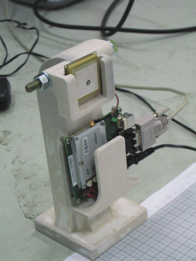
Recently new RFID based (Finkenzeller and Waddington, We tested both linearly and circularly polarized antennas
2003) localization methods have been proposed. Due to in order to determine the one providing the best detection
the highly non-Gaussian noise which characterize these area and radiation pattern. Ideally the detection should
sensors, usually PF (Particle Filter) based methods are not be influenced by the orientation of the tag.
used to estimate the position of a mobile robot (Joho et al., During the characterization experiments we tested differ-
2009; Hahnel et al., 2004; Schneegans et al., 2007) obtain- ent tags, to identify the one providing the widest reading
ing accurate position estimation. These results, however, region, according to our application, and with the smallest
can only be obtained by using a high number of par- dimensions, in order to insert it inside a peg that will be
ticles and by significantly increasing the computational buried in the ground:
burden of the algorithm. For service robot applications,
• UPM RAFLATAC Wet Inlay RAFSEC short-dipole:
like autonomous lawnmowers, the available computational
a rectangular-shaped tag, bigger than the other tested
power is limited for cost reasons. Thus, it is not possible
tags, but with very good performance;
to implement computationally demanding algorithms as
• LAB ID Inlay UH3D40: a square-shaped omnidirec-
particle filters. In (Choi et al., 2010, 2011) a triangulation
tional tag;
based method, where many tags are densely present on the
• LAB ID Inlay UH331: a rectangular-shaped tag;
floor is proposed. In gardening applications, this approach
• LAB ID Inlay UHI4015: the tested tag with smallest
is unfeasible because it would imply to dig a lot of RFID
dimension;
in the garden.
In (Boccadoro et al., 2010) an efficient Constrained The experiment was made in order to identify the com-
Kalman Filter (CKF) is proposed for localizing a mobile bination of devices with the most stable and well-shaped
robot. However it is required that at least one RFID is reading region but also to minimize the power consump-
always detected by the robot. tion and the cost.
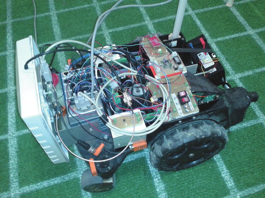
This research is made in cooperation with a company First a support for the RFID reader and antenna was
leading in the production of gardening tools. The goal created with a 3D printer (see Fig. 1). Then we fixed
of this paper is to design a new approach for the local- it at the border of a graph paper sheet. The choice of
ization and the navigation of robotic mowers. We aim at creating the support in chalk was taken according to the
obtaining a uniform mowing of the garden while respecting fact that a metal support could alter the electro-magnetic
the cost budget for extra sensors. The proposed approach field generated by the antenna thus altering its reading
uses a low cost three degrees of freedom IMU (Inertial region and the result of the experiments.
Measurement Unit) and an RFID (Radio-Frequency IDen- The first set of experiments was made with the RFID tags
tification) antenna with an RFID reader to estimate the put on the graph paper. Then we measured the reading
position of the robot through RFID tags placed only on the efficiency η defined as:
border of the working area (the garden). The localization
is obtained extending the CKF proposed in (Boccadoro T ags
et al., 2010) for merging the RFID readings with the η= (1)
Acqs
odometric data coming from the Hall sensors of the wheels
and with the orientation information given by the IMU.
In order to mow the whole garden without leaving un- where T ags is the number of read tags per unit time and
treated areas and to avoid passing too many times on the Acqs is the number of query done by the reader.
same area, we exploit the estimated position for developing Then we repeated the experiment by putting the RFID tag
a planner based on a double blaustrophedon path (two on the mud and repeated all the measurements. Finally we
spirals, one perpendicular to the other), as suggested in dipped the RFID tag in the mud and then repeated all the
(Das et al., 2011) and in (Shiu and Lin, 2008). measurements, to be sure that the RFID system is reliable
even in hard conditions, such as tags covered with mud,
2. RFID SENSOR CHARACTERIZATION dust or grass.
The experiments have shown that the most suitable combi-
It has been shown in Aliberti et al. (2008) that the nation of RFID antenna, reader and tags has been found to
reading region of an RFID in a dry indoor environment be WANTENNAX005 + A528 + UPM RAFLATAC Wet
Inlay RAFSEC short-dipole. We chose a circularly polar-
can be approximated with an ellipse. In the considered
framework, RFID tags will be placed on the border of ized antenna to avoid the dependence of the measurement
a garden, fixed to the perimetral cable that delimits on the orientation of the RFID label. Even with the label
covered with mud and grass, the reading region results
the garden when an automatic lawnmower is used. In
this condition, it can happen that the RFID is covered stable and with only a little smaller dimensions.
by grass, mud or dust. In this section, an experimental The chosen reader could provide to the antenna up to
500mW power, but in order to reduce the power consump-
characterization of the reading region of the RFID under
realistic conditions is presented. tion of the robot and the localization error due to the large
For this experiment we used the RFID reader CAEN RFID dimensions of the reading region, which could increase
the uncertainty in the measurement, we provided only
OEM A528. The antennas we tested are:
200mW during the validation experiments. The resulting
• CAEN WANTENNAX004 (linearly polarized) reading region can be seen in Fig. 2. The red rectangle in
• CAEN WANTENNAX009 (linearly polarized) coordinates (0, 0) represents the position of the antenna.
• CAEN WANTENNAX005 (circularly polarized) The yellow shaded area represents the region from which
• Prototype antenna WANTENNAXVARIOUS (circu- a tag can be detected with 100% efficiency. Here η is
larly polarized) computed with Eq.1.discretized with a granularity much smaller than the one
used for generating the occupancy grid. We indicate with
Λ the set of all the generated cells and with λi = (xi , yi , ϑi )
the i − th cell. Each cell represents a pose from which the
robot can read at least one RFID.
We introduce an n−dimensional binary vector ρ for indi-
cating which tags are read and which are not. If the j − th
tag is detected, then ρ(j) = 1 and otherwise ρ(j) = 0.
For each λi ∈ Λ, we build ρi , namely the binary vector
representing the RFIDs that are detected by the robot
when it stands at the pose λi . The poses λi and the vectors
ρi are stored in a hash-table structure.
Fig. 1. The support used for the characterization of the
RFID devices. 3.2 The localization algorithm
Identification efficiency map
Distance from the antenna [cm]
80 100
The proposed method is differentiated according to
80
whether RFID tags are read or not by the robot. In the
60 first case the algorithm, based on a three step Kalman
60
Filter, makes a prediction according to the model of the
robot (differential drive), it corrects the prediction with
η [%]
40
40
the RFID measurement and then corrects the estimated
position with the last three steps of the Extended Kalman
20
20
Filter doing the measurement update step with the IMU
data. If no RFID is read from the actual position of the
robot, then the algorithm makes the data fusion with a
0 0
−40 −20 0 20 40 simple Extended Kalman Filter (Welch and Bishop, 2006)
Distance from the axis of the antenna [cm] merging the odometric data with the information provided
by the IMU.
Fig. 2. The reading region obtained with A528
RFID reader, WANTENNAX005 antenna and UPM Algorithm 1. Localization Algorithm
Raflatac wet inlay RAFSEC labels.
1 : µ̃k = f µk−1 , uk
3. THE MOWING STRATEGY 2 : Σ̃k = Φk−1 · Σk−1 · ΦTk−1 + Ψk · Rk · ΨTk
3 : ρ = setRho()
We considered the problem of localizing a mobile robot 4 : ρ̄ = ExpSmooth(ρ)
operating in an outdoor environment of known dimension 5 : ρ̃ = getRho(µ̃k , Λ)
with n RFID tags (each with a unique code) placed on its 6 : if (ρ̄ 6= 0) & (ρ̄ 6= ρ̃) then
border at known positions. 7: ∀λi ∈ Λ s.t. ρi = ρ̄:
We exploit the fact that RFID tags can be programmed 7a : P rob(λi ) ∼ (µ̃k , Σ̃k )|λi
to have a unique identification code and a limited area 7b : pi = ε · PXrob(λi )
from where they can be read. When a code is read by 8: µ̂k = λ i · pi
the robot, it can be uniquely associated to an RFID and, λi s.t. ρi =ρ̄
consequently, to its neighbouring region. Furthermore, X T
the robot is endowed with an IMU from which it gets 9: Σ̂k = [λi − µ̂k ] · [λi − µ̂k ] · pi
orientation information. λi s.t. ρi =ρ̄
In the following, the mowing strategy will be illustrated 10 : else
for a differential drive robot, as our prototype. Everything 11 : µ̂k = µ̃k
can be easily extended to robots with different kinematic 12 : Σ̂k = Σ̃k
structures. 13 : endif
14 : K k = Σ̂k · ΓTk · (Γk · Σ̂k · ΓTk + σIM
2
U)
−1
3.1 The off-line set-up 15 : µk = µ̃k + K k · [ϑIM U,k − g (µ̃k )]
16 : Σk = (I − K k · Γk ) · Σ̂k
First of all we discretize the working area (the garden to
be mowed) of the robot using an occupancy grid map, The algorithm is recursive and the k − th step is discussed.
initializing the cells “to be mowed” with low cost values. Lines 1 and 2 are the firsts two steps of the classical
T
The dimensions of the cells are chosen to be a little smaller Extended Kalman Filter: µk = (x, y, ϑ)k is the state
than the dimension of the blade mounted under the robot, vector of the system which represents the position and
T
in order to ensure a small overlap when covering the field. the orientation of the robot at step k, uk = (δR , δL )k
Exploiting the fact that the positions and the reading areas is the input vector with δR and δL the advancements of
of the RFIDs are known, we build a data structure that the right and left wheel respectively. The vector uk is
will be used in the localization algorithm. Let Ar be the characterized by a noise due to the drift of the wheels
reading area of the r − th RFID and let A = ∪nr=1 Ar . Let and is modelled with a gaussian white noise with zero
C be the configuration space of the robot. The set A ∩ C is mean and covariance Rk (Martinelli and Siegwart, 2003).the Extended Kalman Filter takes place. Line 14 computes
The function f µk−1 , uk is the time propagation model
defined as: the Kalman gain, in line 15 the estimated yaw angle of the
robot is corrected by merging the prediction with the data
coming from the IMU. Finally, in line 16, the covariance
δR + δL δR − δL
xk = xk−1 + · cos ϑk−1 + matrix Σk , is updated, in order to keep track of the esti-
2 2d
mation uncertainty. Here g (µ̃k ) is the measurement model
δR + δL δR − δL
f µk−1 , uk = yk = yk−1 + · sin ϑk−1 + function computed with the just obtained estimation of the
2 2d
ϑk = ϑk−1 + δR − δL
orientation, Γk is its Jacobian computed in µk−1 , ϑIM U,k
d is the yaw angle measured by the IMU at the time step k
(2) 2
and σIM U is its variance.
Thus the robot can correct (if it is necessary) its estimated
δR − δL position every time it reaches the border of the working
The term is due to the discretization of the
2d area, while the correction provided by the fusion with
numerical integration via a second-order Runge-Kutta the IMU keeps on correcting the orientation while the
method (Oriolo et al., 2002). robots works in the middle of the garden. The drift of the
Here d is the dimension of the axle of the robot. Given gyroscopes is compensated by stopping the robot during
the time propagation function, let Φk−1 and Ψk be re- its task for few seconds, and then by considering the angle
spectively its Jacobians computed in µk−1 and the input rates registered with the still robot as offsets. This simple
vector uk . Σk−1 is the covariance matrix computed at the strategy has been proven successful in several field tests.
previous step of the algorithm, while Rk is the covariance Using the estimated pose of the robot, a path planning
associated to the input. strategy has been designed for obtaining a smart and
At each step, the antenna searches for neighbouring uniform coverage of the whole lawn. In order to take into
RFIDs. A scan of the ρ vector is then performed (line account possible localization imprecisions that may lead to
3). An element is set to 0 if the corresponding RFID has some uncovered areas, a path consisting of two orthogonal
not been read and to 1 otherwise. In order to avoid false spirals is generated for a square garden. This path is
positive readings, we filter the ρ vector using exponential redundant and it increases the duration of the mowing
smoothing (line 4) as suggested in Boccadoro et al. (2010). task but, at the same time, decreases the possibility of
Thus, we store the value of the ρ string for nw steps in the leaving uncovered areas. This algorithm generates the path
past and we choose a parameter α ∈ (0, 1) for properly to follow by selecting those cells of the occupancy grid in
tuning the smoother and we obtain: which the robot has spent less time, which have a lower
"n −1 #−1 n −1
w w
cost, and then by increasing the cost of those cells in which
X X the robot has already passed through. With respect to the
ρ̄k = αl · αl · ρ(k−l) (3)
random navigation case, by using this method the cutting
l=0 l=0
redundancy is greatly decreased, as well as the energy
where ρk represents the value of the string ρ at time consumption and resulting in a better-looking final shape
k. Furthermore, after the prediction step, it is possible of the lawn. This planning strategy can also be extended to
to estimate the RFIDs that should be detected at the irregularly shaped fields using vertical cell decomposition
configuration µ̃k by using the data structure Λ. We will or other standard techniques (Lavalle, 2006).
indicate the corresponding value of the estimated reading
as ρ̃ (line 5).
4. SIMULATIONS
If some RFIDs are read and if the filtered string of the
read RFIDs ρ̄ and the expected string of RFIDs ρ̃ are
different, it means that µ̃k is inconsistent with the read In this section is illustrated the effectiveness of the pro-
tags and that it can be updated using the detected RFIDs posed localization algorithm through computer simulation.
and the corresponding reading regions. The used computer is a laptop with an Intel Core i3 350M
If the conditions at line 6 of the Algorithm 1 are satisfied, processor with a clock speed of 2.27 GHz and 4GB of
all the poses λi from which the tags corresponding to ρ̄ RAM. We used MATLAB R2010b(64bit) for the simu-
can be read are fetched from the data structure Λ (line 7). lation. The simulated robot moves in a working area of
Each λi represents a possible pose where the robot could (10×10)m with forty tags scattered along its edge (one tag
be, given the reading of the RFIDs. Thus, we associate a each meter). We set nw = 5 and α = 0.99 as parameters
probability of being in each λi by evaluating the multivari- of the exponential smoothing. We used a discretization of
the reading region (as described in Section 3.1) with cells
ate normal distribution with mean µ̃k and covariance Σ̃k
of dimension (50 × 50)mm and π/18 rad.
in λi (line 7a). In line 7b, a weight is associated to each The paths generated can be seen in Fig. 3. The red solid
λi introducing normalizing factor ε. Finally in lines 8 and line represents the estimated path, while the blue dotted
9 we compute the mean and the covariance matrix of the
line represents the simulated ground truth. The yellow star
predicted position updated using the RFIDs. represents the starting position, the red star and the blue
If the conditions at line 6 are not satisfied it means that star represents respectively the final estimated position
either no RFIDs are detected or that the prediction made
and the ground truth. The purple stars are the RFID
using odometry is consistent with the detected tags. In labels. The dark green thick line indicates the border of
both cases the information coming from RFIDs is not
the map.
useful for improving the estimate of the pose. Thus, the
prediction obtained using odometry is used (lines 11 and In Fig. 3(a) the paths generated with the proposed method
12). can be evinced. The robot comes out of the working area
Once the prediction phase is over, the correction step of of only a few cm and the final positions, the ground truthVIEW 2010 (SP1). This controller is provided with an
analog input module (NI9201), an analog output module
10
(NI9263), a digital input module (NI9422) and a RS232
interface module (NI9870).
Under the robot, a three edged blade is used to accomplish
the cutting task. The blade diameter is 25cm. The RFID
Y [m]
antenna and the CompactRIO controller are located on
1
5
the front side of the robot. The 25V battery is located on
the back of the robot.
0
9 10
0
0 5 10
X [m]
(a)
10
Fig. 4. The built prototype.
Y [m]
The experiments took place in a square arena with 2 m side
5
and with eight RFID tags put slightly outside (40 cm) of
the border of the field. The experiments took place on a
synthetic grass carpet.
The RFID antenna reading region, was approximated ac-
0
cording to the results obtained in Section 2 with an ellipse
of semi-axis 250 mm and 350 mm respectively.
−2
0 5 10 12
The map was discretized in an occupancy grid of 10 × 10
X [m] cells (squares of 200 mm side). The dimension of the
(b) cell was decided taking into account the dimension of the
blade of the lawnmower. Thus the robot, during its spiral
Fig. 3. The simulated paths for the proposed method, Fig. shaped movement, partially covers cells in which it has
3(a), and with the “only odometry” localization, Fig. already been, reducing the probability of leaving uncovered
3(b). areas. We set nw = 5 and α = 0.99 as parameters of the
exponential smoothing.
one and the estimated one, are almost overlapping (the The robot starts its task from the middle of the first cell
estimated position is only 185 mm away from the ground and moves along the first spiral. Once it finishes the first
truth and the square mean error between the estimated spiral, it gets back to the starting point and then starts
path according to the ground truth is only 164 mm). moving following the second spiral. Once the robot finishes
As a comparison, we simulated the robot which is local- the second spiral it gets back to the starting point.
izing itself using a dead-reckoning algorithm, i.e. comput- In Fig. 5 the experimental results are shown. The thick
ing its time propagation model using only data given by dark line marks the perimeter of the lawn. White cells
odometry (i.e. the Hall sensors mounted on the wheels). As represent areas where the robot hasn’t passed through,
can be evinced from the pictures (Fig. 3(b)), in the dead- dark green cells represent areas where the robot has passed
reckoning case the robot leaves the working area of several through while doing the first spiral and light green cells
centimetres, and its final position, according to the ground represent those cells where the robot has passed through
truth, is far from the estimated one (about 2119 mm) and during the second spiral. Purple stars represents the po-
the mean square error is 1328 mm. sition of the RFID labels. The yellow star and the black
arrow represents respectively the initial position and ori-
5. EXPERIMENTAL RESULTS entation of the robot.
In Fig. 5(a) the behaviour of the dead-reckoning local-
In order to validate the proposed algorithm, a prototype ization can be seen. The robot moves accordingly to the
lawnmower robot has been built (Fig. 4). The robot has path-planner through the two spirals, but it goes almost
three motors: two brushless DC motors for the wheels and one meter away from the border of the working area. This
a direct drive brushless DC motor for the blade. Each is unacceptable, because regulations (Regulation, 2010)
motor has its own driver. These motors are provided with require that the robot is allowed to leave the assigned area
Hall sensors, which have been used to compute the speed of a maximum distance equal its length. Furthermore the
of each wheel. The used IMU (a Silicon Sensing Pin-Point coverage of the area isn’t satisfactory at all.
Gyro Evaluation Board) has three gyroscopes, one for each We also did an experiment using as localization algorithm
axis, and is fixed on the top of the axle of the robot. an Extended Kalman Filter which merges only the odo-
The high-level control of the robot is performed by the metric information with the IMU data: results are shown
Real-Time controller NI cRIO, programmed with Lab- in Fig. 5(b). In this case, the efficiency of the robot isgreater than the one obtained in the dead-reckoning case. Boccadoro, M., Martinelli, F., and Pagnottelli, S. (2010).
The working area is almost covered, but the robot keeps Constrained and quantized Kalman filtering for an
on going outside of the working area (about 40cm, almost RFID robot localization problem. Autonomous Robots,
the length of the robot). 29(3-4), 235–251.
Finally we repeated the experiment with the robot local- Brooks, R.A. (1986). A Robust Layered Control Syste.
izing itself with the proposed strategy. The robot covers Robotics, (I), 14–23.
the 100% of the working area, and it leaves the assigned Chae, H., Christiand, C., Choi, S., Yu, W., and Cho, J.
map of just few centimetres only when it’s turning. (2010). Autonomous Navigation of Mobile Robot Based
on DGPS/INS Sensor Fusion by EKF in Semi-Outdoor
Structured Environment. Evaluation, 1222–1227.
Choi, B.s., Member, S., Lee, J.w., and Lee, J.j. (2011).
A Hierarchical Algorithm for Indoor Mobile Robots
Localization using RFID Sensor Fusion. System, (c).
Choi, B.s., Member, S., and Lee, J.j.J.w. (2010). An
Improved Localization System with RFID Technology
for a Mobile Robot. Electrical Engineering.
Das, C., Becker, A., and Bretl, T. (2011). Probably
Approximately Correct Coverage for Robots with Un-
certainty. Aerospace Engineering, 1160–1166.
(a) (b) Finkenzeller, K. and Waddington, R. (2003). RFID Hand-
book.
Hahnel, D., Burgard, W., Fox, D., Fishkin, K., and Phili-
pose, M. (2004). Mapping and localization with RFID
technology. IEEE International Conference on Robotics
and Automation, 2004. Proceedings. ICRA ’04. 2004,
1015–1020 Vol.1.
Inaki, R. (2010). Hanging around and wandering on mobile
robots with a unique controller. Sciences-New York, 1–
6.
Joho, D., Plagemann, C., and Burgard, W. (2009). Model-
(c)
ing RFID signal strength and tag detection for localiza-
tion and mapping. 2009 IEEE International Conference
Fig. 5. The coverage of the robot in the case of “only on Robotics and Automation, 3160–3165.
odometry” localization, Fig. 5(a), in the case of sensor Lavalle, S.M. (2006). Planning Algorithms.
fusion with an IMU, Fig. 5(b), and for the proposed Martinelli, A. and Siegwart, R. (2003). Estimating the
localization algorithm, Fig. 5(c). Odometry Error of a Mobile Robot during Navigation.
European Conference on Mobile Robots (ECMR 2003).
6. CONCLUSIONS AND FUTURE WORK Newstadt, G., Green, K., Anderson, D., Lang, M., Morton,
Y., and McCollum, J. (2008). Miami Redblade III: A
In this paper a novel localization algorithm, based on a GPS-aided Autonomous Lawnmower. Journal of Global
modified Constrained Kalman Filter, has been proposed. Positioning Systems, 7(2), 115–124.
Simulations and experiments have been proposed to val- Oriolo, G., De Luca, A., and Vendittelli, M. (2002). WMR
idate the results of the paper. With this new approach control via dynamic feedback linearization: design,
to navigation, autonomous lawnmowers can increase their implementation, and experimental validation. IEEE
life (the lawn is mowed in less time, so the battery life Transactions on Control Systems Technology, 10(6),
lasts longer and mechanical parts are less subject to wear) 835–852.
and their efficiency (better final shape of the garden and Regulation (2010). En 60335-2-107. European Regulation.
less energy consumption) while respecting the cost budget Schneegans, S., Vorst, P., and Zell, A. (2007). Using RFID
imposed by the market. Snapshots for Mobile Robot. Technology, 1–6.
To further test the efficiency of the proposed method, ex- Shiu, B.m. and Lin, C.l. (2008). Design of an autonomous
periments in a wider working area and in areas of irregular lawn mower with optimal route planning. 2008 IEEE
shape will take place. International Conference on Industrial Technology, 1–6.
Future work aims at improving the prototype of the Welch, G. and Bishop, G. (2006). An Introduction to the
robot. Furthermore, the current carrying perimetral wire Kalman Filter. In Practice, 1–16.
surrounding the garden will be explicitly considered and Zhao, H., Chiba, M., Shibasaki, R., Xiaowei, S., Jinshi, C.,
exploited for gaining further insights on the position of the and Hongbin, Z. (2008). Slam in a dynamic large out-
robot and better results in the navigation. door environment using a laser scanner. In Proceedings
of the IEEE Internationa Conference on Robotics and
REFERENCES Automation, 1455 –1462.
Aliberti, R., Di Giampaolo, E., and Marrocco, G. (2008).
A model to estimate the RFID read-region in real envi-
ronments. 2008 38th European Microwave Conference,
(October), 1711–1714.You can also read