ARGSLAB: A TOOL FOR ANALYZING EXPERIMENTAL OR SIMULATED PARTICLE NETWORKS
←
→
Page content transcription
If your browser does not render page correctly, please read the page content below

ArGSLab: A tool for analyzing experimental or
                                                                      simulated particle networks
                                                                              k
                                                     Jasper N. Immink†, ,∗ , J. J. Erik Maris‡ , Ronja F. Capellmann† , Stefan U. Egelhaaf† ,
                                                                     Peter Schurtenbergerk,⊥ , Joakim Stenhammark
                                                      †   Condensed Matter Physics Laboratory, Heinrich-Heine-University Düsseldorf, Düsseldorf, Germany.
                                                                           k Division of Physical Chemistry, Lund University, Lund, Sweden.
                                                              ‡ Inorganic Chemistry and Catalysis Group, Utrecht University, Utrecht, the Netherlands.
                                                          ⊥ Lund Institute of advanced Neutron and X-ray Science (LINXS), Lund University, Lund, Sweden.
                                                                                  ∗ Tel: +49-211 8114327; E-mail: immink@hhu.de

                                                 Microscopy and particle-based simulations are both powerful techniques to study aggregated par-
arXiv:2108.13690v1 [cond-mat.soft] 31 Aug 2021

                                                 ticulate matter such as colloidal gels. The data provided by these techniques often contains infor-
                                                 mation on a wide array of length scales, but structural analysis methods typically focus on the local
                                                 particle arrangement, even though the data also contains information about the particle network
                                                 on the mesoscopic length scale. In this paper, we present a MATLAB software package for quantify-
                                                 ing mesoscopic network structures in colloidal samples. ArGSLab (Arrested and Gelated Structures
                                                 Laboratory) extracts a network backbone from the input data, which is in turn transformed into
                                                 a set of nodes and links for graph theory-based analysis. The routines can process both image
                                                 stacks from microscopy as well as explicit coordinate data, and thus allows quantitative compari-
                                                 son between simulations and experiments. ArGSLab furthermore enables the accurate analysis of
                                                 microscopy data where, e.g., an extended point spread function prohibits the resolution of indi-
                                                 vidual particles. We demonstrate the resulting output for example datasets from both microscopy
                                                 and simulation of colloidal gels, in order to showcase the capability of ArGSLab to quantitatively
                                                 analyze data from various sources. The freely available software package can be used either with
                                                 a provided graphical user interface or directly as a MATLAB script.

                                                 1        Introduction
                                                 Colloidal dispersions exist in many shapes and forms, and understanding their behavior is relevant to bi-
                                                 ological, 1 ecological, 2 and industrial 3 processes. The structures observed in such dispersions include for
                                                 example amorphous colloidal glasses 4 and arrested colloidal gel networks. 5,6 The macroscopic behavior
                                                 of colloidal dispersions is in large part determined by this spatial arrangement, and material properties
                                                 such as the thermal conductivity and rheology vary strongly with the micro- and mesoscopic organi-
                                                 zation of the particles. 7–11 Thus, determining this spatial organization and understanding its link to the
                                                 macroscopic behavior is a major point of interest within soft matter science. 12–14 For example, knowledge
                                                 about the local structure of colloidal particles in gel networks 15–17 has led to the development of models
                                                 that couple the network structure to macroscopic parameters such as the storage modulus. 18 Such mod-
                                                 els often require structural data that describe the gel network over a broad range of length scales, and
                                                 microscopy and numerical simulations both offer powerful tools for probing the formation kinetics and
                                                 structural properties of particle gels on this broad range of length scales. 19–26 These methods are often
                                                 combined with computational analyses that allow for the extraction of structural parameters, 27,28 such
                                                 as pair correlation functions, structure factors, and coordination numbers, that are particularly useful for
                                                 describing the local network structure. 29–32
                                                 Applying these analyses to experimental and computational datasets, 14,33,34 valuable insight regarding
                                                 the local structure of such particle networks can be gained. However, such datasets also contain struc-
                                                 tural information on longer length scales, although a limited number of tools exist that can analyze the
                                                 datasets reliably and efficiently. 35,36 Existing analysis tools primarily focus on quantifying the material
                                                 thickness and porosity of the network. These analyses however require well-resolved individual network
                                                 segments, which is not always available when analyzing microscopy data due to limitations in image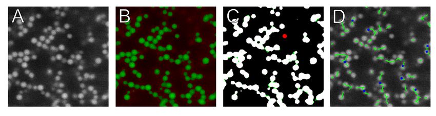
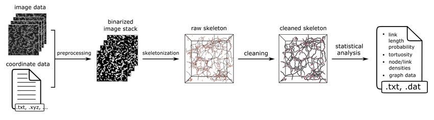
resolution, especially with small particles. 37–39
In this Article, we will present a versatile computational method called ArGSLab, Arrested and Gelated
Structures Laboratory, developed as a MATLAB package providing a set of tools to quantitatively ana-
lyze network structures in particle aggregates such as colloidal gels. ArGSLab performs a mesoscopic
structural analysis that uses experimental or computational data to reconstruct three-dimensional gel
networks 40 as graphs of nodes and links. 39 ArGSLab furthermore enables quantification of the network
structure using mesoscopic structural parameters such as node densities, branching densities and branch
length statistics. As input, ArGSLab handles both image stacks from microscopy and sets of particle co-
ordinates from either experiment or simulation. Crucially, the software does not require microscopy data
containing well-resolved particle positions, enabling the analysis of structures formed by particles down
to the same size range as the point-spread function. The software then converts the input data into
single voxel-thin backbone structures, using routines based on established algorithms. 41–43 The gener-
ated network structures are then transformed into a set of nodes and links for further statistical, graph
theory-based analysis and visualization. ArGSLab can be accessed either via the provided graphical user
interface (GUI) or directly through the MATLAB script.
In the following, we will first summarize the main features of ArGSLab and briefly discuss the overall
workflow. Then, we will discuss the algorithms in some detail, and thereafter discuss the different output
options. Finally, we will illustrate the capabilities of the software using three different data sets: (i) a
set of microscopy images of colloidal gels with well-resolved particles, (ii) similar data but with poorly
resolved individual particles, and (iii) coordinate sets from Brownian dynamics simulations.

2    Software description

Figure 1: Overview of the ArGSLab workflow. As input, the software uses either image stacks or particle coordinate
sets, which are preprocessed into binarized images and then transformed into “skeletons”. These go through a
cleaning step, and are then transformed into a set of nodes and links for quantitative analysis. ArGSLab provides a
histogram of the link lengths, the density of nodes and links in the system, and the tortuosity of the network.

An overview of the general ArGSLab workflow is shown in Fig. 1. The four major stages of the analysis
are: (i) preprocessing, (ii) skeletonization, (iii) cleaning and (iv) quantitative analysis. In the preprocess-
ing stage, coordinate sets are first transformed into image stacks, which are then successively Gaussian
blurred, binarized and morphologically closed. Small unconnected structures are then removed, and
small holes are filled. The skeletonization stage consists of the iterative erosion of voxels that belong
to the material network, until a single-voxel thick backbone skeleton remains. This is then transformed
into a graph of nodes and links. The cleaning stage removes artefacts from the skeletonization process,
and the fourth and final stage contains a thorough analysis of the graph, producing statistics such as link
length distribution, tortuosity and node density. In the following, we will describe these features.
2.1    Algorithms
As input, the package accepts either .tiff image stacks from confocal microscopy or 3D particle coordinate
sets from, e.g., computer simulations. Coordinate diagrams are first projected onto a .tiff image stack
using user-defined voxel dimensions, with an optional convolution using a default or user-defined point
spread function. The user-provided or generated image stacks are then treated with a Gaussian blur
and binarized (i.e., transformed into images containing only black or white pixels). The purpose of
treating images with a Gaussian blur is to reduce noise in the final skeleton, predominantly in the form
of unrealistically small side chains, a known artefact of this type of skeletonization. 42,44 The binarization
step is performed with a threshold individually calculated for each image slice. Determination of the
threshold can be done either manually or using automated routines, where the automatic determination
uses Otsu’s method, 45 whereas the manual method determines, for each slice, the intensities I10 and
I90 , which are the pixel intensity values below which 10% and 90% of individual pixel intensities fall,
respectively. A user-defined value Vu between 0 and 1 then defines the threshold intensity IT , with
                                           IT = I10 +Vu (I90 − I10 ).                                     (1)
The threshold determination is performed on each slice individually in order to compensate for differ-
ences in signal intensities between image slices: this is helpful when investigating microscopy data where
a scattering length density mismatch leads to the average fluorescence intensity being dependent on the
focal depth in the sample, or where fluorescence bleaching effects play a role. 37 Images are then treated
with a morphological closing step, consisting of subsequent dilation and erosion steps 46 performed with
a user-defined ellipsoidal structural element. This procedure removes noise and effectively fills small
gaps between particles, ensuring contiguity where necessary. 47 Structures are connected should their bi-
narized shapes be closer than twice the structural element radius. Subsequently, unconnected clusters
smaller than a threshold fraction are removed, with larger unconnected clusters being analyzed as sepa-
rate network structures. Finally, holes in the structure that are enclosed on all sides in 3D and are smaller
than a user-defined threshold value are detected and filled in, reducing unphysical holes in the skeleton.
The sizes of the Gaussian blur kernel, the morphological closing element and the minimal cluster size
take either default or user-defined values.
Subsequently, the package performs the skeletonization, using algorithms adapted from Kollmannsberger
et al. 43 This process consecutively removes material voxels bordering non-material voxels, with the con-
dition that they are not end points, non-Euler invariant points, and are Euler simple points. Removal of
a voxel considers the 3×3 voxel cube D3 (i) surrounding voxel i, i.e. a cube of 27 voxels with voxel i at
the center. An end point is defined as the case where D3 (i) contains in total two material voxels, of which
one is i. Euler invariant points are defined as voxels that, upon removal, do not lead to a change of the
Euler characteristic of the total structure. 48–50 We define an Euler simple point as a voxel i whose removal
neither changes the connectivity nor the Euler characteristic of D3 (i); 48,51 a more detailed discussion of
these definitions can be found in Lee et al. 42 The transformation of a skeleton into a graph of nodes
and links is then performed by assuming that (i) each voxel i whose surrounding D3 (i) contains exactly
2 material voxels is an end node, (ii) each voxel i whose D3 (i) contains exactly 3 material voxels belongs
to a link and (iii) each voxel i whose D3 (i) contains more than 3 material voxels is a branching node.
While the skeletonization process robustly extracts the relevant backbone structure, several known unre-
alistic features can arise, often due to noisy or irregular data. 42 The subsequent cleaning steps remove
such unwanted features, and are performed iteratively using the following procedures:
  1. Unphysically small side chains, arising from irregular structure surfaces, 42,52 are excluded by re-
     moving all side chains smaller than a certain threshold value, by default set to 1.5σ with σ the
     particle diameter.
  2. The removal of canal nodes, i.e. nodes that are connected to exactly two links. Such nodes and their
     connecting links are effectively one single link and therefore merged.
  3. Nodes that are in close proximity are collected into a single node, as dense sections of gels with
     irregular edges often lead to complex and unphysical skeleton sections with many interconnected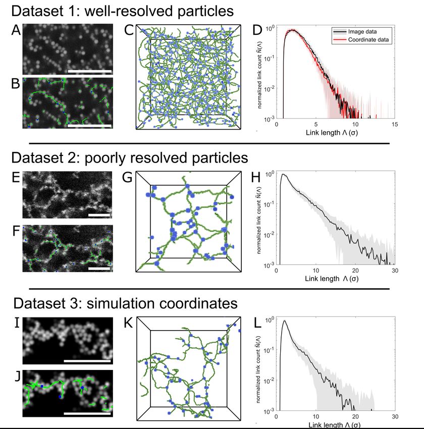
nodes and links. A set of nodes to be collected contains all nodes that are closer than a threshold
      value to another node in the same set. The threshold value is by default set to 0.9σ .

After these procedures, a new skeleton is formed from the cleaned graph.

Figure 2: Visualized output. A) slices of the original image .tiff stack overlaid with the skeleton (green) and branch-
ing nodes (blue). Since these are 2D slices of a 3D image, interrupted skeleton strands continue in adjacent z-slices.
B) 3D rendering of the same skeleton.

2.2    Visualization
ArGSLab provides output that allows the user to visualize and quantify the analyzed network structures.
The software also provides output that helps optimizing the parameters of the skeletonization process.
The standard visualizations are: (i) the original image stack overlaid with the calculated skeleton and
branching nodes, as shown in Fig. 2A (data from Kohl et al. 34 ), and (ii) a fully rotatable 3D rendering of
the skeleton backbone, as shown in Fig. 2B. 53,54
As described in Section 2.1, several parameters and thresholds can be changed from their default val-
ues to optimize the output. The package provides several types of visualization to help optimize those
parameters, a selection of which are shown in Fig. 3. Starting from a raw image stack (Fig. 3A), a new
image stack is output after the binarization step (Fig. 3B). This is intended to help setting the binarization
threshold, should the automatic method be insufficient. Fig. 3C shows the effects of further preprocessing
after binarization, i.e. the morphological closing, hole filling, and the removal of smaller unconnected
structures. The final results are shown in Fig. 3D, showing an overlay of the raw image with the final
skeleton.

2.3    Statistical analysis
From the graph of branching nodes and connecting links, a number of statistical quantities can be ex-
tracted, such as the number and density of nodes and links. The total number of nodes and links NN and
NL are calculated together with the average number of links per node NNNL . The density of nodes and links
ρN and ρL respectively are given in units of µm−3 and σ −3 with σ the particle diameter. Furthermore,
ArGSLab provides a histogram showing the distribution of link lengths in the network, presenting the nor-
malized link count Ñ(Λ) as a function of link length Λ, which we define as the length of a link between
two nodes as measured along the link path. Ñ(Λ) is related to the fractal dimension d f , a parameter
often used for characterizing aggregated systems: 7,55,56 a propensity for long links and low d f are both
characteristic of open aggregates. Another output measure is the tortuosity ξ , which is defined as the
average trajectory length following a backbone strand λ , divided by the calculated Euclidean distance
λEuc between their start and end points A and B:

                                                   λ (A,B)
                                            ξ=                 ,                                       (2)
                                                  λEuc (A,B)
Figure 3: Slices from 3D input and a selection of ArGSLab’s output image stacks. A) Raw input image. B) Raw input image overlaid with a green and red color filter, produced in the binarization step. Green indicates voxels determined to contain material (material voxels), and red to contain no material (non-material voxels). Black voxels had little to no intensity in the original image. C) Preprocessing effects after binarization: white sections are material voxels, unaltered by the preprocessing, green sections are material voxels added by preprocessing, and red sections are previous material voxels that have been removed. D) Overlay of the raw data with the final skeleton and nodes. where A and B are the start and end points of paths along the backbone intersecting respectively the upper and the lower box face in either Cartesian direction, and the angular brackets denote averaging over all such paths for a given configuration. ξ provides a measure of the strand erraticity, 39,57–59 and is often used in catalysis, 60 blood vessel analysis, 61 or satellite geography. 59 All quantitative analyses are corrected for box edge effects. Furthermore, additional analyses beyond the ones described here are facilitated by ArGSLab as the skeleton backbone and the node and link lists can be exported as .mat or .txt files, after which analyses tailored to the specific system can be applied. 2.4 Graphical User Interface The package can be accessed either using the provided MATLAB wrapper code, or using the graphical user interface (GUI), shown in Fig. 4. The GUI gives intuitive access to the full capabilities of the code and requires only a few inputs: the folder path containing the input data, the number of z-slices to be analyzed in each file (in case not all slices should be analyzed), the voxel dimensions, and the average particle diameter. Ticking the “fine-tuning options” box reveals several further options that allow for op- timization of output quality and can typically be left at their default values. These are described in-depth in the GUI tooltip menus and the package manual. The GUI is designed to be an intuitive tool for using ArGSLab, allowing users to run the full analysis without loss of functionality as compared to the wrapper script. 3 Examples In the following we will illustrate the use of ArGSLab by showing the processing of three example datasets. Dataset 1 consists of microscopy images of a set of colloidal gels made from PMMA spheres with an added depletant that causes attractive forces leading to gel formation. The gels are imaged using confocal laser scanning microscopy (CLSM) and the large particles allow for individual particles to be well-resolved. 34 The results from analyzing this dataset are compared to the corresponding results from coordinate sets of the particle centers, extracted using routines following Crocker and Grier. 27 Dataset 2 contains CLSM images of gels of smaller, pNIPAm microgel particles (as described in Section 5) that cannot be individ- ually resolved. Dataset 3 is a set of particle coordinates obtained from Brownian dynamics simulations of colloidal gels formed from colloidal particles with attractive patches icosahedrally arranged on the particle surface. 39 Further details about the preparation can be found in Section 5, and the results are summarized in Fig. 5 and Table 1.
Figure 4: Screenshot of the GUI, with fine-tuning tools enabled.

Figs. 5A-D show the results for Dataset 1. The quantitative analyses in Fig. 5D and Table 1 reflect the sim-
ilarity between experimental skeletons and the ones obtained from the corresponding coordinate data.
The small discrepancies between the results can be explained as follows: the coordinate extraction rou-
tines identify the vast majority of particles, but atypical particles, due to synthetic or imaging anomalies,
are sometimes not picked up. While this only leads to negligible errors in tracking experiments, ArGSLab’s
structural analysis identifies this as broken links. Such effects can also arise from the determination of a
particle center slightly off from its real particle center due to experimental noise. ArGSLab can partially
accommodate such anomalies by choosing larger structural element sizes.
The results from Dataset 2 (Figs. 5E-H and Table 1) clearly demonstrate the software’s ability of extracting
quantitative data from structures constructed from non-resolvable particles. Nonetheless, the lower data
quality often leads to the need for a more careful selection of optimization parameters. Skeletonization of
data with low contrast, low signal-to-noise ratio, or poor z-resolution is known to lead to skeletons with
small, unphysical side chains, or with a multitude of nodes in dense cluster-like sections. 42 Tuning the
parameters of the cleaning routines can alleviate these types of noise: larger Gaussian blurring kernels or
morphological closing structural elements often cause dense clusters to be correctly interpreted as closed
entities. Furthermore, the node collection threshold in the second cleaning step can be increased, col-
lecting these virtual nodes into a single node. Furthermore, the terminal branch length threshold (third
cleaning step in Section 2.1) can be raised to remove unphysical side chains. Changing these parameters
can affect the number of nodes and links found, and should be kept constant between datasets for full
comparability. In all our examples we have used the default parameters, which provides optimal compa-
rability between different experiments.
One important consideration when setting the analysis parameters is that determining whether two parti-
cles are to be considered in contact or not is a non-trivial question 62–64 which will affect the final skeleton.
Whether ArGSLab considers two segments in contact or not is implicitly governed by the binarization and
the morphological closing steps. In brief, two gel segments will be considered in contact if their material
voxels after binarization are closer together than the diameter of the morphological closing element. This
choice is rationalized by considering that colloidal gels require a significant attractive potential, and in-
Table 1: Values from statistical analysis of the example datasets in Fig. 5.

               Type                          ρN [σ −3 ]      ρL [σ −3 ]      NL /NN     ξ
               Dataset 1 (images)            7.86 × 10⁻²     1.34 × 10⁻¹     1.70       2.03 ± 0.14
               Dataset 1 (coordinates)       8.36 × 10⁻²     1.44 × 10⁻¹     1.72       2.05 ± 0.09
               Dataset 2                     7.18 × 10⁻³     8.67 × 10⁻³     1.22       2.23 ± 0.12
               Dataset 3                     9.10 × 10⁻³     1.02 × 10⁻²     1.13       2.25 ± 0.13

tersegment gaps are often metastable, while noisy images often lead to apparent gaps. Optimal skeleton
output therefore requires a careful tuning of the morphological closing element size and the binarization
threshold, with the preselected standard parameters as good starting points.
The results from Dataset 3 (Figs. 5I-L and Table 1) further demonstrate that ArGSLab offers a direct com-
parison between experimental systems and model systems studied by simulations. The large difference
in the node and link densities ρN and ρL between Dataset 1 and Datasets 2 and 3 results from the much
higher volume fraction in the former system (φ = 0.2 compared to φ = 0.05) that leads to much higher
node and link densities in Dataset 1. The difference in φ also results in a significantly lower Ñ(Λ) at high
Λ for Dataset 1, and the tortuosity ξ is also lowered by the higher ρN . It is also apparent that the gels in
Datasets 2 and 3 have a stronger propensity for having end nodes rather than branching nodes from the
lower NL /NN ratios in Table 1.

4    Conclusions and Perspectives
In this Paper, we have demonstrated the capabilities of ArGSLab, a tool for analyzing networks of ag-
gregated particulate matter, such as colloidal gels. We have shown that ArGSLab is able to analyze both
microscopy and simulation data, and allows for direct comparison between different datasets. The soft-
ware provides a quantitative analysis of the mesoscopic network structure, which is more difficult to
analyze than the local particle arrangements. Importantly, ArGSLab also provides a method to quan-
tify systems where individual particles are not resolvable and the local structure thus cannot easily be
probed. The graph theory approach that our package applies enables comprehensive analyses of ag-
gregated structures, and it yields several parameters allowing for a unique insight into their structure.
Moreover, ArGSLab can be used to transform experimental or simulation data into a set of nodes and links
for further analysis, and thus provides powerful information for the development of new analyses tailored
to user-specific needs. Since the method is developed to analyze any network that is composed of smaller
segments, ArGSLab can be applied to networks beyond colloidal gels, such as protein networks, 66 bac-
terial aggregates in biofilms 67 and biological cell networks. 68 By providing for an easy means to extract
global network parameters, ArGSLab provides a powerful method of extracting mesoscopic structural pa-
rameters that can be related to microscopic and macroscopic properties, for instance obtained from light
scattering or rheology.

5    Materials and Methods
Dataset 1 is the same as dataset C5 in Ref. 34. Particles are PMMA spheres with a diameter σ = 1.72µm,
aggregated due to depletion forces. We analyze 30 stacks with total imaged volume 8.85 × 104 µm3 or
1.72 × 10⁴ σ 3 per stack, voxel dimensions of 0.061×0.061×0.12 σ 3 , and a volume fraction φ of approxi-
mately 0.2. Further details can be found in Ref. 34.
Dataset 2 consists of polystyrene/poly-N-Isopropylacrylamide core-shell microgels, synthesized using a
method described in Ref. 65. In collapsed form, σ = 398nm and particles aggregate irreversibly due
to a combination of van der Waals interactions and other short-range attractions. We analyzed 40 im-
age stacks with a total imaged volume per stack of 1.08 × 104 µm3 or 1.71 × 10⁵ σ 3 , voxel dimensions of
0.054×0.054×0.12 σ 3 , with φ = 0.05. The samples are prepared and imaged using identical methods as
described in Ref. 39.
Figure 5: Analysed data from the three example datasets: A-D) Dataset 1, corresponding to dataset C5 in Ref. 34. E- H) Dataset 2, containing particle gels formed by attractive microgel particles, synthesized as in Ref. 65 I-L) Brownian dynamics simulation data of particles with patchy attractions, from Ref. 39. Panels (A,E,I) show image sections from the raw data, panels (B,F,J) overlays of the same image and the final skeleton, panels (C,G,K) 3D renderings of the full skeleton (green) and branching nodes (blue), and panels (D,H,L) the normalized link length distribution Ñ(Λ). The two datasets in panel (D) corresponds to Ñ(Λ) obtained using either the raw image data, or from a particle coordinate set extracted from the same data, demonstrating the equivalence of the two approaches. All 3D skeleton renderings correspond to a volume of approximately 1.7 ×10⁴ σ 3 , and the scale bars represent 10σ .
Dataset 3 was obtained from Brownian dynamics using particles with attractive patches icosahedrally
placed on the surface as described in Ref. 39. We analyze the final structures from four different Brow-
nian dynamics simulations. To compensate for local fluctuations, the results from 10 temporally close
coordinate diagrams were averaged for each simulation. The total system volume was 1.0 × 10⁵ σ 3 with
φ = 0.05. Further details can be found in Ref. 39.

Computational Efficiency
On an Intel® octacore i7-7700 CPU with 3.60 GHz running Windows 10 and MATLAB 2021a, extracting
a skeleton and subsequent analysis from one image from dataset 1 (512x512x151 pixels, φ = 0.2) takes
approximately 5 minutes. Starting from the coordinate diagram only adds a few seconds to this calcu-
lation time. Additional visualization and optimization visualization adds 6 minutes. The code has been
tested on iOS, Windows and Linux platforms, with comparable computation times. Decreasing image
size and φ reduces computational time.

Resources
A project page for the package exists at GitHub.com (github.com/jimmink/argslab), where the standalone
MATLAB package and GUI for Windows, iOS and Linux are freely available, together with a user manual
and example datasets. An idealized, computer-generated image stack is also available, intended to help
users familiarize themselves with ArGSLab and its parameters. A walkthrough of the analysis of this
image is available as Supplementary Information.

Acknowledgements
We gratefully acknowledge financial support from the Alexander von Humboldt Foundation (JNI), the
European Research Council (ERC-339678-COMPASS (PS)) and the Swedish Research Council (Grant
numbers 2018-04627 (PS) and 2019-03718 (JS)).

Supplementary Information
A walkthrough of the ArGSLab analysis of the freely available benchmarking image.

References
 [1] C. Don, W. Lichtendonk, J. J. Plijter, and R. J. Hamer. Glutenin macropolymer: a gel formed by glutenin particles. J. Cereal
     Sci., 37(1):1 – 7, 2003.

 [2] A. B. Burd and G. A. Jackson. Particle aggregation. Ann. Rev. Mar. Sci., 1(1):65–90, 2009.

 [3] A. H. Alexopoulos and C. Kiparissides. On the prediction of internal particle morphology in suspension polymerization of
     vinyl chloride. part i:: The effect of primary particle size distribution. Chem. Eng. Sci., 62(15):3970 – 3983, 2007.

 [4] G. L. Hunter and E. R. Weeks. The physics of the colloidal glass transition. Reports on Progress in Physics, 75(6):066501, 2012.

 [5] W. C. K. Poon, A. D. Pirie, and P. N. Pusey. Gelation in colloid–polymer mixtures. Faraday Discuss., 101:65–76, 1995.

 [6] V. Trappe and P. Sandkühler. Colloidal gels—low-density disordered solid-like states. Current Opinion in Colloid and Interface
     Science, 8(6):494–500, 2004.

 [7] W.-H. Shih, W. Y. Shih, S.-I. Kim, J. Liu, and I. A. Aksay. Scaling behavior of the elastic properties of colloidal gels. Phys. Rev.
     A, 42:4772–4779, 1990.

 [8] W. J. Tseng and K. C. Lin. Rheology and colloidal structure of aqueous tio2 nanoparticle suspensions. Mater. Sci. Eng. A, 355
     (1):186 – 192, 2003.

 [9] M. Laurati, G. Petekidis, N. Koumakis, F. Cardinaux, A. B. Schofield, J. M. Brader, M. Fuchs, and S. U. Egelhaaf. Structure,
     dynamics, and rheology of colloid-polymer mixtures: From liquids to gels. J. Chem. Phys., 130(13):134907, 2009.

[10] N. Shalkevich, A. Shalkevich, and T. Bürgi. Thermal conductivity of concentrated colloids in different states. J. Phys. Chem.
     C, 114(21):9568–9572, 2010.
[11] T. Gibaud, A. Zaccone, E. Del Gado, V. Trappe, and P. Schurtenberger. Unexpected decoupling of stretching and bending
modes in protein gels. Phys. Rev. Lett., 110:058303, 2013.
[12] E. Dickinson. Structure and rheology of colloidal particle gels: Insight from computer simulation. Adv. Colloid Interface Sci.,
199-200:114 – 127, 2013.
[13] J. D. Park, K. H. Ahn, and N. J. Wagner. Structure-rheology relationship for a homogeneous colloidal gel under shear startup.
J. Rheol., 61(1):117–137, 2017.
[14] K. A. Whitaker, Z. Varga, L. C. Hsiao, M. J. Solomon, J. W. Swan, and E. M. Furst. Colloidal gel elasticity arises from the
packing of locally glassy clusters. Nat. Commun., 10:2237, 2019.
[15] C. P. Royall, S. R. Williams, T. Ohtsuka, and H. Tanaka. Direct observation of a local structural mechanism for dynamic arrest.
Nat. Mater., 7:556–561, 2008.
[16] J. M. van Doorn, J. Bronkhorst, R. Higler, T. van de Laar, and J. Sprakel. Linking particle dynamics to local connectivity in
colloidal gels. Phys. Rev. Lett., 118:188001, 2017.
[17] J. de Graaf, W. C. K. Poon, M. J. Haughey, and M. Hermes. Hydrodynamics strongly affect the dynamics of colloidal gelation
but not gel structure. Soft Matter, 15:10–16, 2019.
[18] H. Wu and M. Morbidelli. A model relating structure of colloidal gels to their elastic properties. Langmuir, 17(4):1030–1036,
2001.
[19] P. Varadan and M. J. Solomon. Direct visualization of flow-induced microstructure in dense colloidal gels by confocal laser
scanning microscopy. Journal of Rheology, 47(4):943–968, 2003.
[20] A. I. Campbell, V.J. Anderson, J. S. van Duijneveldt, and P. Bartlett. Dynamical arrest in attractive colloids: The effect of
long-range repulsion. Phys. Rev. Lett., 94:208301, 2005.
[21] Y. Gao, J. Kim, and M. E. Helgeson. Microdynamics and arrest of coarsening during spinodal decomposition in thermore-
versible colloidal gels. Soft Matter, 11:6360–6370, 2015.
[22] R. Massaro, G. Colombo, P. van Puyvelde, and J. Vermant. Viscoelastic cluster densification in sheared colloidal gels. Soft
Matter, 16:2437–2447, 2020.
[23] B. H. Bijsterbosch, M. T. A. Bos, E. Dickinson, J. H. J. van Opheusden, and P. Walstra. Brownian dynamics simulation of
particle gel formation : From argon to yoghurt. Faraday Discuss., 101:51–64, 1995.
[24] A. M. Puertas, M. Fuchs, and M. E. Cates. Comparative simulation study of colloidal gels and glasses. Phys. Rev. Lett., 88:
098301, 2002.
[25] Q. Zhang, D. Bahadur, E. M. Dufresne, P. Grybos, P. Kmon, R. L. Leheny, P. Maj, S. Narayanan, R. Szczygiel, S. Ramakrishnan,
and A. Sandy. Dynamic scaling of colloidal gel formation at intermediate concentrations. Phys. Rev. Lett., 119:178006, 2017.
[26] P. Padmanabhan and R. N. Zia. Gravitational collapse of colloidal gels: non-equilibrium phase separation driven by osmotic
pressure. Soft Matter, 14:3265–3287, 2018.
[27] J. C. Crocker and D. G. Grier. Methods of digital video microscopy for colloidal studies. J. Colloid Interf. Sci., 179(1):298 –
310, 1996.
[28] A. D. Dinsmore, E. R. Weeks, V. Prasad, A. C. Levitt, and D. A. Weitz. Three-dimensional confocal microscopy of colloids.
Appl. Opt., 40(24):4152–4159, 2001.
[29] K. Masschaele, J. Fransaer, and J. Vermant. Flow-induced structure in colloidal gels: direct visualization of model 2d suspen-
sions. Soft Matter, 7:7717–7726, 2011.
[30] L. C. Hsiao, R. S. Newman, S. C. Glotzer, and M. J. Solomon. Role of isostaticity and load-bearing microstructure in the
elasticity of yielded colloidal gels. Proc. Natl. Acad. Sci. U.S.A, 109:16029–16034, 2012.
[31] B. D. Leahy, N. Y. C. Lin, and I. Cohen. Quantitative light microscopy of dense suspensions: Colloid science at the next decimal
place. Curr. Opin. Coll. Int. Sci., 34:32 – 46, 2018.
[32] Z. J. Glover, C. Ersch, U. Andersen, M. J. Holmes, M. J. Povey, J. R. Brewer, and A. C. Simonsen. Super-resolution microscopy
and empirically validated autocorrelation image analysis discriminates microstructures of dairy derived gels. Food Hydrocoll.,
90:62 – 71, 2019.
[33] E. Zaccarelli, P. J. Lu, F. Ciulla, D. A. Weitz, and F. Sciortino. Gelation as arrested phase separation in short-ranged attractive
colloid–polymer mixtures. Journal of Physics: Condensed Matter, 20(49):494242, 2008.[34] M. Kohl, R. F. Capellmann, M. Laurati, S. U. Egelhaaf, and M. Schmiedeberg. Directed percolation identified as equilibrium
pre-transition towards non-equilibrium arrested gel states. Nat. Commun., 7:11817, 2016.
[35] E. Dàvila, M. Toldrà, E. Saguer, C. Carretero, and D. Parés. Characterization of plasma protein gels by means of image analysis.
LWT - Food Sci. Technol., 40(8):1321 – 1329, 2007.
[36] Z. Ruff, S. H. Nathan, R. R. Unwin, M. Zupkauskas, D. Joshi, G. P. C. Salmond, C. P. Grey, and E. Eiser. Designing disordered
materials using dna-coated colloids of bacteriophage fd and gold. Faraday Discuss., 186:473–488, 2016.
[37] M. C. Jenkins and S. U. Egelhaaf. Confocal microscopy of colloidal particles: Towards reliable, optimum coordinates. Adv.
Coll. Int. Sci., 136(1):65 – 92, 2008.
[38] B. Huang, M. Bates, and X. Zhuang. Super-resolution fluorescence microscopy. Annu. Rev. Biochem., 78(1):993–1016, 2009.
[39] J. N. Immink, J. J. E. Maris, P. Schurtenberger, and J. Stenhammar. Using patchy particles to prevent local rearrangements in
models of non-equilibrium colloidal gels. Langmuir, 36:419–425, 2020.
[40] M. Tateno and H. Tanaka. Numerical prediction of colloidal phase separation by direct computation of navier–stokes equation.
Npj Comput. Mater., 5:40, 2019.
[41] S. Lobregt, Verbeek P. W., and F. C. A. Groen. Three-dimensional skeletonization: Principle and algorithm. IEEE Trans. Pattern
Anal. Mach. Intell., PAMI-2(1):75–77, 1980.
[42] T. C. Lee, R. L. Kashyap, and C. N. Chu. Building skeleton models via 3-d medial surface axis thinning algorithms. CVGIP -
Graph. Model. Im., 56(6):462 – 478, 1994.
[43] P. Kollmannsberger, M. Kerschnitzki, F. Repp, W. Wagermaier, R. Weinkamer, and P. Fratzl. The small world of osteocytes:
connectomics of the lacuno-canalicular network in bone. New J. Phys., 19(7):073019, 2017.
[44] A. Leborgne, J. Mille, and L. Tougne. Noise-resistant digital euclidean connected skeleton for graph-based shape matching.
Journal of Visual Communication and Image Representation, 31:165 – 176, 2015.
[45] N. Otsu. A threshold selection method from gray-level histograms. IEEE T. Syst. Man Cy. B, SMC-9:62–66, 1979.
[46] E.R. Dougherty. An Introduction to Morphological Image Processing. Books in the Spie Tutorial Texts Series. SPIE Optical
Engineering Press, 1992. ISBN 9780819408457.
[47] D. Legland, K. Kiêu, and M.-F. Devaux. Computation of minkowski measures on 2d and 3d binary images. Image Anal.
Stereol., 26(2), 2011.
[48] C. Pudney. Distance-ordered homotopic thinning: A skeletonization algorithm for 3d digital images. Comput. Vis. Image
Underst., 72(3):404 – 413, 1998.
[49] M. A. Miller, R. Blaak, and J.-P. Hansen. Topological characteristics of model gels. Journal of Physics: Condensed Matter, 22
(10):104109, 2010.
[50] P. K. Saha, G. Borgefors, and G. Sanniti di Baja. A survey on skeletonization algorithms and their applications. Pattern
Recognit. Lett., 76:3 – 12, 2016.
[51] W. Abu-Ain, S. N. H. S. Abdullah, B. Bataineh, T. Abu-Ain, and K. Omar. Skeletonization algorithm for binary images. Procedia
Technology, 11:704–709, 2013.
[52] P. K. Saha, D. Jin, Y. Liu, G. E. Christensen, and C. Chen. Fuzzy object skeletonization: Theory, algorithms, and applications.
IEEE Trans. Vis. Comput. Graphics, 24(8):2298–2314, 2018.
[53] J. Ahrens, B. Geveci, and C. Law. Paraview: An end-user tool for large-data visualization. In The Visualization Handbook,
2005.
[54] J. Yeh. vtkwrite: Exports various 2d/3d data to paraview in vtk file format. (https://github.com/joe-of-all-trades/vtkwrite),
GitHub., 2020. Retrieved August 27, 2020.
[55] M. Lattuada, H. Wu, A. Hasmy, and M. Morbidelli. Estimation of fractal dimension in colloidal gels. Langmuir, 19(15):
6312–6316, 2003.
[56] S. Lazzari, L. Nicoud, B. Jaquet, M. Lattuada, and M. Morbidelli. Fractal-like structures in colloid science. Adv. Colloid Interface
Sci., 235:1 – 13, 2016.
[57] M. P. Hollewand and L. F. Gladden. Modelling of diffusion and reaction in porous catalysts using a random three-dimensional
network model. Chem. Eng. Sci., 47(7):1761 – 1770, 1992.[58] P. Xu, B. Yu, Y. Feng, and Y. Liu. Analysis of permeability for the fractal-like tree network by parallel and series models.
Physica A, 369(2):884 – 894, 2006.
[59] G. Connor-Streich, A. J. Henshaw, J. Brasington, W. Bertoldi, and G. L. Harvey. Let’s get connected: A new graph theory-based
approach and toolbox for understanding braided river morphodynamics. WIREs Water, 5(5):e1296, 2018.
[60] Y. Wang, G. Sun, J. Dai, G. Chen, J. Morgenstern, Y. Wang, S. Kang, M. Zhu, S. Das, L. Cui, and L. Hu. A high-performance,
low-tortuosity wood-carbon monolith reactor. Adv. Mater., 29(2):1604257, 2017.
[61] K. M. Kliś, R. M. Krzyżewski, B. M. Kwinta, K. Stachura, Marek Moskała, and K. A. Tomaszewski. Computer-aided analysis of
middle cerebral artery tortuosity: association with aneurysm development. J. Neurosurg, 130(5):1478 – 1484, 2018.
[62] J. Brujić, C. Song, P. Wang, C. Briscoe, G. Marty, and H. A. Makse. Measuring the coordination number and entropy of a 3d
jammed emulsion packing by confocal microscopy. Phys. Rev. Lett., 98:248001, 2007.
[63] M. C. Jenkins, M. D. Haw, G. C. Barker, W. C. K. Poon, and S. U. Egelhaaf. Finding bridges in packings of colloidal spheres.
Soft Matter, 7:684–690, 2011.
[64] S. Pradeep and L. C. Hsiao. Contact criterion for suspensions of smooth and rough colloids. Soft Matter, 16:4980–4989, 2020.
[65] J. N. Immink, M. J. Bergman, J. J. E. Maris, J. Stenhammar, and P. Schurtenberger. Crystal-to-crystal transitions in binary
mixtures of soft colloids. ACS Nano, 14(11):14861–14868, 2020.
[66] M. Jekle and T. Becker. Dough microstructure: Novel analysis by quantification using confocal laser scanning microscopy.
Food Research International, 44(4):984–991, 2011.
[67] L. C. Powell, M. F. Pritchard, E. L. Ferguson, K. A. Powell, S. U. Patel, P. D. Rye, S.-M. Sakellakou, N. J. Buurma, C. D. Brilliant,
J. M. Copping, G. E. Menzies, P. D. Lewis, K. E. Hill, and D. W. Thomas. Targeted disruption of the extracellular polymeric
network of pseudomonas aeruginosa biofilms by alginate oligosaccharides. NPJ Biofilms Microbiomes, 4:13, 2018.
[68] B. Andrée, H. Ichanti, S. Kalies, A. Heisterkamp, S. Strauß, P.-M. Vogt, A. Haverich, and A. Hilfiker. Formation of three-
dimensional tubular endothelial cell networks under defined serum-free cell culture conditions in human collagen hydrogels.
Sci. Rep., 9:5437, 2019.You can also read


