AUDITORY CORTICAL REPRESENTATION AND ITS CLASSSIFICATION FOR PASSIVE SONAR SINGNALS
←
→
Page content transcription
If your browser does not render page correctly, please read the page content below
The 21st International Congress on Sound and Vibration
                                              13-17 July, 2014, Beijing/China

     AUDITORY CORTICAL REPRESENTATION AND ITS
     CLASSSIFICATION FOR PASSIVE SONAR SINGNALS
     Lixue Yang, Kean Chen
     Department of Environment Engineering, Northwestern Polytechnical University, Xi’an,
     China 710072
     e-mail: yanglixue.2008@163.com

     This study presents an auditory cortical representation for passive sonar signal and use it to
     extract features to categorize an unknown signal as being of man-made or natural origin. A
     ridge partial least squares (RPLS) model is given to establish the decision criterion, and re-
     gression coefficients are used to search for salient regions of the auditory cortical representa-
     tion related to the classification task. In order to verify the utility of this method, some per-
     ceptual features motivated by music timbre research are used as predicators, and it is shown
     that the recognition accuracy of such an auditory cortical representation is slightly higher.
     Some acoustical analysis based on such two methods draw a conclusion that passive sonar
     signals of natural origin tend to possess more rhythmic transients or stationary noise.

1.     Introduction
      Automatic classification for passive sonar signals plays a significant role in modern naval war,
in which feature extraction is a crucial step that determines recognition accuracies. While features
based on traditional signal processing technologies have achieved some success, the final decision
in practice still depends on aural judgment of sonar operators. Therefore, extracting features in-
spired by auditory principles has attracted more and more attentions1, 2.
      A direct method is to build analytical auditory models and extracting salient features based on
their representations. A typical auditory model involves two stages: periphery and central process-
ing. All models incorporate a realistic cochlear component in periphery stage, and they mainly dif-
fer with respect to further central processing that occurs and the degree to which this is constrained
by physiology and anatomy. The model proposed by Shamma incorporate auditory representations
at the level of primary auditory cortex based on multi-scale spectro-temproal modulations3. The
model has been proven useful in assessment of speech intelligibility4, discrimination of speech from
non-speech signals5, mapping unpleasantness of sounds6, and modeling of underwater noises tim-
bre7.
       This research will select the final representation of Shamma’s model as predictors to classify
unknown sonar signals as being of either man-made or natural origins. Although practical tasks can
be more refined than this, it is ultimately this classification that is of interest to the Navy, as it dis-
tinguished things that can kill you (e.g. enemy ships and submarines) from things cannot (e.g. dol-
phins and whales). A RPLS method8 that combines PLS and logistic regression is used as classifier,
and regression coefficients intuitively display the salient regions of auditory representations related
to classification. Some perceptual features9 motivated by music timbre research will be extracted in
order to validate this method and aid in acoustical analysis.

ICSV21, Beijing, China, 13-17 July 2014                                                                  1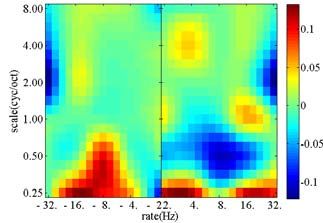
21st International Congress on Sound and Vibration (ICSV21), Beijing, China, 13-17 July 2014
2. Method
This section will show how to get the auditory cortex representations of sonar signals, and use
the ridge partial least squares (RPLS) method to map them into man-made or natural origins.
2.1 Sonar records
All the sonar records are download form Historic Naval Ships Association. There are totally
100 sonar signals, in which 50 come from man-made origins, and 50 are made by natural origins.
Here, man-made origins include some ships, submarines and torpedoes, while natural origins may
be some natural phenomenon (rain, earthquake, ice and bubbles etc.) and creature vocalizations
(whale, dolphin, fish and snapping shrimp etc). The length of each sound file is set to 5s.
2.2 Auditory cortical model
This model is based on neurophysiological, biophysical, and psychoacoustical investigations
at various stages of the auditory system3. It consists of two basic stages. An early stage models the
transformation of the acoustic signal into an internal neural representation (Auditory Spectrogram).
A central stage analyzes the spectrogram to estimate the content of its spectral and temporal modu-
lations (Figure 1).
Figure 1. Schematic of the auditory processing3.
The early stages of auditory processing are modelled as a sequence of three operations. The
acoustic signal entering the ear produces a complex spatiotemporal pattern of vibrations along the
basilar membrane of the cochlea. The basilar membrane outputs are then converted into inner hair
cell intra–cellular potentials. This process is modelled as a 3–step operation: a high pass filter (the
fluid–cilia coupling), followed by an instantaneous nonlinear compression (gated ionic channels),
and then a low pass filter (hair cell membrane leakage). Finally, a lateral inhibitory network detects
discontinuities in the responses across the tonotopic axis of the auditory nerve array.
Higher central auditory stages (especially the primary auditory cortex) further analyze the
auditory spectrum into more elaborate representations, interpret them, and separate the different
cues and features associated with different sound precepts. Specifically, from a conceptual point of
view, these stages estimate the spectral and temporal modulation content of the auditory spectro-
gram. They do so computationally via a bank of modulation-selective filters centred at each fre-
quency along the tonotopic axis. It has a spectro-temporal impulse response (usually called Spectro-
Temporal Response Field-STRF) in the form of a spectro-temporal Gabor function which effec-
tively results is a multi-resolution wavelet analysis of auditory spectrogram.
In summary, this model translates a signal x(t ) to a 4-dimensional cortical representa-
tion R ( F , , , t ) , in which F denotes central frequency (Hz), and are temporal modulation rate
(Hz) and spectral modulation scale (cycles/octave) respectively. For our purpose here, the time-
averaged representations are taken as predictors.
ICSV21, Beijing, China, 13-17 July 2014 2
21st International Congress on Sound and Vibration (ICSV21), Beijing, China, 13-17 July 2014
2.3 Ridge partial least squares (RPLS)
Logistic regression is a good choice of classifier for binary classification (0 for man-made ori-
gin and 1 for natural origin in this case), and with regression coefficients salient features can be
displayed intuitively. We often use iteratively reweighed least squares (IRLS) method to obtain the
maximum likelihood (ML) estimates of coefficients, but it can’t converge when the number of ob-
servations n (100 sonar signals) is large smaller than feature dimensions p (the cortical representa-
tion has 128 frequency channels, 10 rates and 6 scales, that is totally 7680 predictors). In this situa-
tion, dimension reduction is needed first.
The method of partial least squares (PLS) has been found to be a useful dimension reduction
technique10, which chooses a small number of latent variables (linear combination of the p predic-
tors) that have maximum covariance with response variables. A direct application of PLS to logistic
regression seems to be intuitively unappealing because PLS handles continuous responses. In order
to extend PLS to logistic regression, we can replace the binary response vector y with a pseudo-
response z variable whose expected value has linear relationship with the covariates, but it in re-
turn cause for IRLS method.
In order to reconcile this contradiction, Fort and Lambert8 propose a new procedure which
combine Ridge penalty - the regularization step- and PLS - the dimension reduction step - and so
called Ridge-PLS (RPLS). Let be some positive real constant and be some positive integer,
RPLS divides in two steps:
1. RIRLS(y, X , ) ( z , W ) . On the basis of IRLS method, RIRLS method exert a penalty
term on the maximum likelihood function, where is ridge parameter that controls the degree of
penalty.
2. WPLS( z , X , W , ) ˆ PLS, . WPLS is a weighted PLS procedure with weight W , in
which is the number of latent variables and ˆ PLS, is the corresponding estimation value of re-
gression coefficients.
A detailed implementation can be found in Ref 8. RPLS depends on two parameters, and .
is determined at the end of Step 1, as minimizing the BIC criterion, and is usually determined
based on 5-fold cross-validation method. This paper set ridge parameter range from 0.1 to 1000, and
will be any positive integer between 1 and 10.
2.4 Data pre-processing
Although the RPLS procedures can handle a large number (thousands) of variables, the dimen-
sions of auditory model may be still too large for practical use. Furthermore, a considerable per-
centage of variables do not show differential expression across groups and only a subset of vari-
ables is of interest. We perform the preliminary selection of variables on the basis of the ratio of
their between-groups to within-groups sum of squares11. For a variable j, this ratio is
BSS ( j ) i k I ( yi k )( xkj x. j )
2
k 0,1 (1)
WSS ( j ) i k I ( yi k )( xij xkj ) 2
Where x. j denotes the average value of variable j across all samples and xkj denotes the average
value of variable j across samples belonging to class k. We selected predictors with the largest 1000
BSS/WSS ratios.
3. Sonar signal classification and analysis
Primary music timbre researches reveal a lot of perceptual features, which reflect signal struc-
ture differences between different sounds, or describe some special subjective feelings, and they
ICSV21, Beijing, China, 13-17 July 2014 321st International Congress on Sound and Vibration (ICSV21), Beijing, China, 13-17 July 2014
have been used into various target classification tasks10. Therefore, we can expect that the combina-
tion of these perceptual features can also be able to distinguish different sonar targets. In the follow-
ing, we will use them to do the same work, compare the result with it of auditory cortical represen-
tation, and combine them to do some auditory analysis of sonar signals related to classification.
3.1 Perceptual features
In this paper, perceptual features motivated by music timbre research are extracted using MIR
Toolbox 1.4, and they can be classified into four categories:
Temporal: RMS Energy, Low-Energy Ratio, Zero Crossings, Attack Time and Attack Slope;
Spectral: Spectral Centroid, Spectral Spread, Spectral Skewness, Spectral Kurtosis, Spectral
Rolloff, Spectral Entropy, Spectral Flatness, Spectral Irregularity and Roughness;
Spectro-temporal: Spectral Flux;
Rhythm: Fluctuation, Tempo Rate.
This paper extracts all the instantaneous features using a window length of 50ms and an over-
lap of 50% between successive windows. Since most sonar signals in this research are stationary,
the mean of each feature across all windows is retained.
3.2 Comparison of results
Then we will compare the performance of auditory cortical representation and perceptual fea-
tures in sonar signal classification task. The average recognition accuracies of 100 times of 5-fold
cross-validation are plotted against the number of latent variables in Figure 2, and ridge parameter
is set to 0.1 based on BIC statistics. The best accuracy of auditory cortical representation (the green
line) is slightly better than that of perceptual features (the blue line).
0.82
average recognition accuaracies
0.8
0.78
0.76
0.74
0.72
0 2 4 6 8 10
number of latent variables
Figure 2. Average recognition accuracies of two methods
Since no research does this automatic classification task like this, this result can’t be used for
horizontal comparison with other methods. However, Collier asked sonar operators and sonar-naïve
people to do a similar task, in which sonar operators achieved 81% correct and the novices, 74%
correct12. Although there is no overlap between sonar recordings used in these two researches, we
can speculate that the auditory cortical representation can achieve almost same performance with
sonar operators.
3.3 Auditory analysis
. After evaluating the classification performance, we can get the final classifier model based
on the whole sample set. This model presents regression coefficient of each feature or component,
ICSV21, Beijing, China, 13-17 July 2014 421st International Congress on Sound and Vibration (ICSV21), Beijing, China, 13-17 July 2014
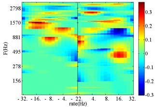
and the bigger ones are more related to classification. The regression coefficients in the auditory
cortical representation are shown in figure 3, in which coefficients are projected into frequency-rate,
scale-frequency and scale-rate plane respectively. In this research, the sound which has bigger val-
ues in red regions may come from natural origins, and the one which has bigger values in blue re-
gions may tend to be man-made origins. From figure 3, we can conclude that:
Figure 3. Regression coefficients distribution in auditory cortex representation
(1) Natural origins tend to have more energy in high frequency regions, particularly be-
tween 500-2000 Hz.
(2) Natural origins tend to have more energy in low scale regions, and this means their
spectrum tend to be more broad and flat.
(3) Natural origins tend to have more energy either in slow or fast modulation rate re-
gions, and these sounds tend to have a very slow or very fast rhythmic transients.
The second model based on perceptual features shows that attack slope, spectral spread, spec-
tral flatness and spectral irregularity have high positive coefficients. High attack slope correspond to
transients (like ice flow, and creature vocalization), and these kind of sounds usually have very slow
(mammal vocalizations) or very fast rhythmic repetition (fish vocalizations). These sounds also
have broader spectrums, which correspond to larger spectral spread. Some natural phenomenon
sounds tends to be noise-like (like rain squall, water flow and earthquake), and they possess large
valued of spectral flatness and spectral irregularity.
In summary, auditory analysis of sonar signals based on these two methods have many simi-
larities. We can conclude that sonar signals of natural origin tend to possess more rhythmic tran-
sients or stationary noise.
4. Summary and conclusion
Classifying an unknown sonar signal as being of man-made or natural origin is an interest is-
sue of Navy. This research attempts to utilize an auditory cortical representation to achieve auto-
matic recognition. In order to overcome the drawback of high dimension of this representation, this
research utilize a RPLS method that combines PLS and logistic regression as classifier and regres-
sion coefficients can be used for auditory analysis. Some perceptual features motivated by music
timbre research are also used as predictors for comparison, and the performance of auditory cortical
representation is better. Finally we do some auditory analysis based on such two methods, and find
many similarities between them. It concludes that sonar signals of natural origin tend to possess
more rhythm transients or stationary noise.
The application of auditory cortical representation into passive sonar signals has achieved
some degree of success. Compared to traditional auditory perceptual features, it is a more complete
description of signal properties by incorporating multi-scale spectro-temproal modulations. Since
this auditory model is developed for speech analysis initially, we should do some refinement for
sonar signals in the future research.
ICSV21, Beijing, China, 13-17 July 2014 521st International Congress on Sound and Vibration (ICSV21), Beijing, China, 13-17 July 2014
REFERENCES
1
Howard, J. H. Psychophysical structure of eight complex underwater sounds, Journal of the
Acoustic Society of America, 62 (1): 149-156, (1977).
2
Tucker, S. and Brown, G. J. Classification of transient sonar sounds using perceptually moti-
vated features. IEEE Journal of Oceanic Engineering, 30 (3): 588-560, (2005).
3
Shamma, S. Encoding sound timbre in the auditory system. IETE Journal of Research, 49 (2):
1-12, (2003).
4
Chi, T., Gao, Y. J., Guyton, M. C., et al. Spectro-temporal modulation transfer functions and
speech intelligibility, Journal of the Acoustic Society of America, 106 (5): 2719-2732, (1999).
5
Mesgarani, N., Slaney, M., and Shamma, S. A. Discrimination of speech from nonspeech
based on multiscale spectro-temporal modulations. IEEE Transactions on Audio, Speech and
Language Processing, 14 (3): 920-930, (2006).
6
Kumar, S., Forster. H. M., Bailey, P., et al. Mapping unpleasantness of sounds to their audi-
tory representation. Journal of the Acoustic Society of America, 124 (6): 3810-3817, (2008).
7
Yang, L. X., Chen, K. A., Wu, Y. Timbre representation and property analysis of underwater
noise based on a central auditory model. Acta Physica Sinica, 62 (19): 194302, (2013).
8
Fort, G., and Lambert-Lacroix, S. Classification using partial least squares with penalized lo-
gistic regression. Bioinformatics, 21 (7), 1104-1111, 2005.
9
Alluri, V., and Toiviainen, P. Exploring perceptual and acoustical correlates of polyphonic
timbre. Music Perception, 27 (3), 223-241, (2009).
10
Herrera-Boyer, P., Peeters, G., Dubnov S. Automatic classification of musical instrument
sounds. Journal of New Music Research, 32 (1), 1-21, (2003).
11
Barker, M., and Rayens, W. Partial least squares for discrimination. Journal of chemometrics,
17: 166-173, (2003).
12
Collier, G. L. A comparison of novices and experts in the identification of sonar signals.
Speech Communication, 43: 297-310, 2004.
ICSV21, Beijing, China, 13-17 July 2014 6You can also read