Bayesian Imputation with Optimal Look-Ahead-Bias and Variance Tradeoff - arXiv
←
→
Page content transcription
If your browser does not render page correctly, please read the page content below
Bayesian Imputation with Optimal Look-Ahead-Bias and Variance
                                                                                                 Tradeoff∗
                                                                   †
                                                 Jose Blanchet            Fernando Hernandez ‡   Viet Anh Nguyen                       §
                                                                                                                                              Markus Pelger¶
                                                                                        Xuhui Zhang‖
arXiv:2202.00871v1 [stat.ME] 2 Feb 2022

                                                                                             January 31, 2022

                                                                                                   Abstract

                                                      Missing time-series data is a prevalent problem in finance. Imputation methods for time-
                                                  series data are usually applied to the full panel data with the purpose of training a model for a
                                                  downstream out-of-sample task. For example, the imputation of missing returns may be applied
                                                  prior to estimating a portfolio optimization model. However, this practice can result in a look-
                                                  ahead-bias in the future performance of the downstream task. There is an inherent trade-off
                                                  between the look-ahead-bias of using the full data set for imputation and the larger variance in
                                                  the imputation from using only the training data. By connecting layers of information revealed
                                                  in time, we propose a Bayesian consensus posterior that fuses an arbitrary number of posteriors
                                                  to optimally control the variance and look-ahead-bias trade-off in the imputation. We derive
                                                  tractable two-step optimization procedures for finding the optimal consensus posterior, with
                                                  Kullback-Leibler divergence and Wasserstein distance as the measure of dissimilarity between
                                                  posterior distributions. We demonstrate in simulations and an empirical study the benefit of
                                                  our imputation mechanism for portfolio optimization with missing returns.

                                          Keywords: Imputation, missing data, look-ahead-bias, Bayesian consensus posterior, Kullback-
                                          Leiber divergence, Wasserstein distance, portfolio optimization
                                          JEL classification: C02, C11, C22, G11

                                             ∗
                                               We gratefully acknowledge the financial support and feedback of MSCI and its data science team. Material in this paper is
                                          based upon work supported by the Air Force Office of Scientific Research under award number FA9550-20-1-0397. Additional
                                          support is gratefully acknowledged from NSF grants 1915967, 1820942, 1838676, and also from the China Merchant Bank.
                                             †
                                               Stanford University, Department of Management Science & Engineering, Email: jose.blanchet@stanford.edu.
                                             ‡
                                               Stanford University, Department of Management Science & Engineering, Email: fhernands01@gmail.com
                                             §
                                               Stanford University, Department of Management Science & Engineering, Email: viet-anh.nguyen@stanford.edu
                                             ¶
                                               Stanford University, Department of Management Science & Engineering, Email: mpelger@stanford.edu.
                                             ‖
                                               Stanford University, Department of Management Science & Engineering, Email: xuhui.zhang@stanford.edu.
1    Introduction
Missing time-series data is a prevalent problem in finance. Its role is becoming even more critical due
to the vast amount of data that is being collected nowadays and the reliance on data driven analytics.
Financial data can be missing for a variety of reasons, which include for example infrequent trading
due to illiquidity, mixed frequency reporting or improper data collection and storage. How this
missing data is handled has substantial impact on any down-stream task in risk management.
A standard approach is to impute missing data. There is a growing body of literature (Little
and Rubin, 2002; van Buuren, 2012) and over 150 practical implementations available (Mayer,
Josse, Tierney, and Vialaneix, 2019) that handle the issue of imputing missing data. However, the
implications of imputation for a downstream out-of-sample task have been neglected so far.
    This paper studies the imputation of missing data in a panel which is subsequently used for
training a model for a downstream out-of-sample task. Our leading example is the imputation of
missing returns prior to estimating a portfolio optimization model. Imputation methods are usually
applied to the full panel to impute missing values. However, this practice can result in a look-ahead-
bias in the future performance of the downstream task. Typically, a machine learning or portfolio
optimization down-stream task splits the panel data into a train-validation-test set according to
the time-ordering of underlying events. Training corresponds to the left-most block portion of the
panel, validation corresponds to a block in the middle of the panel, and testing is done in a block
at the right end of the panel. The “globally observed data” is the entire available panel data set
representing all the data collected during the entire time horizon. Meanwhile, “locally observed
data” refers in our discussion to data available up to a certain time in the past (e.g. the training
section of the panel data set). A standard imputation procedure in practice is to apply a given
imputation tool at hand using the globally observed data. While being natural for the purpose
of reducing error in the imputation, ignoring the time-order of a future downstream task poses a
problem, which is of particular importance for portfolio optimization. Portfolio selection procedures
are designed to exploit subtle signals that can lead to favorable future investment outcomes. A
global imputation is likely to create a spurious signal due to the correlation between training and
testing data induced by the imputation. The training portion of the downstream task itself can
(and often will) pickup the spurious signal created by the imputation procedure, thus giving a false
sense of good performance. For example, if the mean return of an asset is large on the testing data,
a global imputation might increase the estimated mean on the training data and bias the stock
selection. This is an example of an overfitting phenomenon created by “looking into the future”
which investors have to mitigate. In summary, even if the portfolio analysis is done “properly
out-of-sample” on the full panel of imputed values, the look-ahead-bias from the imputation can
render the results invalid.
    Our paper provides a new conceptual perspective by connecting the imputation with a down-
stream out-of-sample task. There is an inherent trade-off between the look-ahead-bias of using the
full data set for imputation and the larger variance in the imputation from using only the training
data. As far as we know, this paper is the first to introduce a systematic approach to study this

                                                  1
trade-off. We propose a novel Bayesian solution which fuses the use of globally observed data (i.e.
data collected during the full time horizon) and locally observed data (i.e. data collected up to a
fixed time in the past) in order to optimize the trade-off between look-ahead-bias (which increases
when using globally observed data to impute) and variance (which increases when using only local
data to impute). More specifically, we connect layers of information revealed in time, through a
Bayesian consensus posterior that fuses an arbitrary number of posteriors to optimally control the
variance and look-ahead-bias trade-off in the imputation.
   The use of statistical and machine learning methods in finance has usually been very careful
in avoiding a look-ahead-bias in the downstream task for a given financial panel without missing
values. For example, Gu, Kelly, and Xiu (2020) and Chen, Pelger, and Zhu (2019) train their
machine learning methods on the training data in the first part of the sample to estimate trading
strategies and evaluate their performance on the out-of-sample test data at the end of the sample.
They follow one common approach in the literature to use only information from the training data
to impute missing information. Their results could potentially be improved by better imputed
values in the training data if those have a sufficiently small look-ahead-bias. In contrast, Giglio,
Liao, and Xiu (2021) impute a panel of asset returns with matrix completion methods applied to
the full panel of assets returns. Hence, their subsequent out-of-sample analysis of abnormal asset
returns has an implicit in-sample component as future returns have been used in the imputation.
These two cases of full data imputation (with look-ahead-bias and small variance) and conservative
imputation (without look-ahead- bias and with large variance) are both special cases of our Bayesian
approach. Each of them corresponds to a different posterior. Our framework allows us to obtain a
“consensus” posterior that is optimal in the sense of this trade-off. Hence, it can be optimal to use
at least some future information if it has a negligible effect on the look-ahead-bias. This becomes
particularly relevant if the amount of missing data on the training data is large.
   As mentioned earlier, we provide the first systematic framework for evaluating look-ahead-bias
and for optimizing the the trade-off between look-ahead-bias and variance in imputations for future
downstream tasks. Any reasonable formulation of this problem needs to consider three ingredients.
First, a representative downstream task that captures stylized features of broad interest. Second, a
reasonable way to fuse or combine imputation estimators which are obtained using increasing layers
of time information. And, finally, a way to connect the first and second ingredients to optimally
perform the desired bias-variance trade off. The objective is to find a way to systematically produce
these three ingredients in a tractable and flexible way. To this end, we adopt a Bayesian impu-
tation framework. This allows us to precisely define look-ahead-bias as deviation from a specific
performance related to a reasonable downstream task, which we take to be optimizing expected
returns in portfolio selection. The expected return is computed with the baseline posterior distri-
bution obtained using only locally observed information. As it is standard in Bayesian imputation
(Little and Rubin, 2002; Rubin, 1987), we impute by sampling (multiple times) from the posterior
distribution given the observed entries by creating multiple versions of imputed data set which can
be used to estimate the optimal posterior return. Our theoretical results focus on the fundamental

                                                 2
case of estimating mean returns in order to clearly illustrate the novel conceptual ideas, but can
be generalized to more general risk management objectives.
   The second ingredient involves a way to fuse inferences arising from different layers of informa-
tion. Our Bayesian approach is convenient because we can optimally combine posterior distributions
using a variational approach, namely, the weighted Barycenter distribution (i.e. the result of an in-
finite dimensional optimization problem which finds a consensus distribution which has the minimal
combined discrepancy among a non-parametric family of distributions based on a given discrepancy
criterion). We use the (forward and backward) Kullback-Leibler divergences and the Wasserstein
distance as criteria to obtain three different ways to generate optimally fused posterior distributions
corresponding to different layers of information (indexed by time). These optimally fused distribu-
tions are indexed by weights (corresponding to the relative importance given to each distribution
to be combined). It is important to note that since our fusing approach is non-parametric, this
method could be used in combination with other downstream tasks and is not tied to the particular
choice that we used in our first ingredient.
   Finally, the third ingredient in our Bayesian method minimizes the variance of the optimal
return strategy (using the expected return as selection criterion) assuming a consensus distribution
given by the second ingredient - therefore indexed by the weights attached to each of the posteriors.
The optimization is performed over the such weights under a given look-ahead-bias constraint. The
constrain parameter can be chosen via cross validation or by minimizing the estimated mean squared
error over all consensus posteriors as a function of the constrain parameter.
   In sum, the overall procedure gives the optimal utilization of different information layers in
time, based on a user-defined bias-variance trade-off relative to the chosen downstream task, and
using an optimal consensus mechanism to fuse the different layers of information.
   We illustrate our novel conceptual framework with the data generating distribution Zt = θ + t ,
where θ is the mean parameter constant over time and t are the noise terms. For example,
in modeling financial returns, assuming time-stationarity (in particular a constant mean) over
moderate time horizons is a common practice in finance (Tsay, 2010). The noise t can in general
follow an AR(p) process. A suitable joint prior on θ is imposed, after which the joint posterior
conditional on observed entries can in principle be calculated. We aggregate the different posteriors
corresponding to different layers of information using the variational approach prescribed by a set of
weights. This set of weights is further optimized to find the optimal consensus posterior according to
a bias-variance criterion. This additional step of optimization over importance weights differentiates
our work from the usual Bayesian fusion setup, as most of the literature only considers a fixed choice
of the weights (Dai, Pollock, and Roberts, 2021; Claici, Yurochkin, Ghosh, and Solomon, 2020).
   To make the two-step optimization procedure tractable, we assume that the noise t are i.i.d
Gaussian with a known covariance matrix and use conjugate prior distributions. This assumption
makes the posterior of the missing entries a conditional Gaussian with mean sampled from the
posterior of θ, and thus we consider only aggregating the different posteriors of θ. We provide
tractable reformulations of the two-step optimization procedure using the forward KL divergence

                                                  3
and Wasserstein distance, when imposing an additional simultaneous diagonalizability condition
on the covariance matrices of the individual posteriors. While our reformulation using backward
KL divergence does not require simultaneous diagonalizability, the resulting optimization problem
is non-convex and may not be scalable. We thus advocate using the forward KL divergence and
Wasserstein distance over the backward KL divergence, unless the simultaneous diagonalizability
condition is seriously violated for the type of data at hand.
   The contributions of this paper can be summarized as follows:

  1. We propose a novel conceptual framework to formalize and quantify the look-ahead-bias in the
     context of panel data imputation. We combine different layers of additional future information
     used in the imputation via optimal non-parametric consensus mechanisms among Bayesian
     posterior distributions in a way that optimally provides a trade-off between the look-ahead-
     bias and the variance.
  2. We illustrate the conceptual framework with a data generating distribution that has a con-
     stant mean vector over time. We propose a two-step optimization procedure for finding the
     optimal consensus posterior. The first step of optimization deals with finding the best pos-
     sible (non-parametric) distribution that summarizes the different posterior models given a
     set of importance weights. The second step of optimization concerns with finding the opti-
     mal weights, based on a bias-variance criterion that minimizes the variance while explicitly
     controlling the degree of the look-ahead-bias.
  3. To make the two-step procedures tractable, we further assume the noise is i.i.d multivariate
     Gaussian with known covariance matrix and use a conjugate prior distribution. Moreover,
     we discuss using the (forward and backward) KL-divergence and Wasserstein distance as the
     measure of dissimilarity between posterior distributions. We advise against the backward
     KL divergence unless in situations where the simultaneous diagonalizability condition on the
     covariance matrices of the individual posteriors is drastically violated.

   Finally, we empirically validate the benefits of our methodology with the downstream task of
portfolio optimization. We show that the use of an optimal consensus posterior results in better
performance of the regret of out-of-sample testing returns measured by what we call “expected
conditional mean squared error”, compared to the use of naive extreme posteriors (corresponding
to focusing either using only the training part of the data for imputation or the full panel data for
imputation). In our companion paper Blanchet, Hernandez, Nguyen, Pelger, and Zhang (2021),
we illustrate the framework to a special case involving the Wasserstein interpolation of these two
extreme posteriors. We show that the many more layers of additional information to be fused result
in better out-of-sample performance compared to Blanchet, Hernandez, Nguyen, Pelger, and Zhang
(2021). We demonstrate the power of our method on both simulated and real financial data, and
under different practically relevant missing patterns including missing at random, dependent block
missing, and missing by values.
   This paper focuses on the finance setting in which handling missing data is particularly preva-
lent, but the distinction between globally and locally observed data is important in other time-series

                                                  4
data as well, for example in electronic health records. Importantly, it generalizes beyond the time-
series setting to data sets with network structure, where each sample corresponds to a vertex in the
network. The globally observed data is the entire collection of vertices in the network, while the
locally observed data is a subset of the vertices defined by a neighborhood in this network. One
may use the locally observed data as the training data set for a relevant downstream task while
using the globally observed data for testing. The vertices that are inside of the neighborhood could
potentially have a causal effect (with respect to a downstream task) on vertices outside, but the
causality in the other direction is not permitted. Such a framework can be used as an approximate
model for, e.g, the prediction of crime rates in different parts of a state, of the radiation level of
surrounding cities after a damage of nuclear power plant, or of the earthquake magnitude in a
geographic region. If missing data is imputed globally using all information, an out-of-sample per-
formance of the downstream task will inherently suffer from overfitting as the imputation extracts
undesirable information. The imputation using only locally observed data again fails to utilize all
valuable information to improve the variance.
    This paper is organized as follows. In Section 2 we discuss the related literature on imputation
methods. In Section 3 we extend the bias-variance multiple imputation framework to more than
two individual posteriors along with two basic modules of the framework: the posterior generator
and the multiple imputation sampler. Section 4 discusses the consensus mechanism module which
complements our framework. Subsequently, in Section 5 and 7, we use the forward and the backward
KL divergence as a measure of dissimilarity between distributions and derive a reformulation of
the consensus mechanism, while in Section 6 we use the Wasserstein distance. Section 8 reports
the simulation and empirical results. The Appendix collects the proofs and additional empirical
results.

2    Related Literature
Strategies for missing data imputation can be classified into two categories: single and multiple
imputation. Single imputation refers to the generation and usage of a specific number (i.e., a
best guess) in place of each missing value. Standard non-parametric methods for single imputa-
tion include k-nearest neighbor, mean/median imputation, smoothing, interpolation and splines
(Kreindler and Lumsden, 2006). Alternatively, single imputation can also be achieved using a
parametric approach such as the popular EM algorithm of Dempster, Laird, and Rubin (1977),
Bayesian networks (Lan, Xu, Ma, and Li, 2020) or t-copulas and transformed t-mixture models
(Friedman, Huang, Zhang, and Cao, 2012). Single imputation also includes the use of iterative
methods in multivariate statistics literature to deal with missing values encountered in classical
tasks such as correspondence analysis (de Leeuw and van der Heijden (1988)), multiple correspon-
dence analysis, and multivariate analysis of mixed data sets (Audigier, Husson, and Josse, 2016).
Recently, there is a surge in the application of recurrent neural networks for imputation, as well as

                                                  5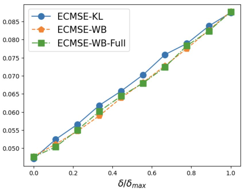
generative adversarial networks.1
       A closely related field of single imputation of panel data is matrix completion and matrix
factorization.2 Chen, Fan, Ma, and Yan (2019) propose a de-biased estimator and an optimal
construction of confidence intervals/regions for the missing entries and the low-rank factors. Xiong
and Pelger (2019) impute missing data with a latent factor model by applying principal component
analysis to an adjusted covariance matrix estimated from partially observed panel data. They
provide an asymptotic inferential theory and allow for general missing patterns, which can also
depend on the underlying factor structure. This is important as Bryzgalova, Lettau, Lerner, and
Pelger (2022) show in their comprehensive empirical analysis, that missing patterns of firm specific
and asset pricing information are impacted by the cross- and time-series dependency structure in
the data. Bai and Ng (2020) suggest an imputation procedure that uses factors estimated from a
tall block along with the re-rotated loadings estimated from a wide block.
       Multiple imputation generalizes the single imputation procedures in that the missing entries are
filled-in with multiple guesses instead of one single guess or estimate, accounting for the uncertainty
involved in imputation. The use of multiple imputation results in m (m > 2) completed data sets,
each is then processed and analyzed with whatever statistical method can be used as if there is no
missing data. Rubin’s rule (Rubin, 1987) is often used to combine the quantity of interest computed
from each completed data set, which averages over the point estimates and uses a slightly more
involved expression for the standard errors.
       The central idea underpinning the multiple imputation is the Bayesian framework. This frame-
work samples the missing values from a posterior predictive distribution of the missing entries
given the observed data. Multiple imputation is first developed for non-responses in survey sam-
pling (Rubin, 1987). Since then, it has been extended to time-series data (Honaker and King,
2010; Halpin, 2016), where a key new element is to preserve longitudinal consistency in imputation.
More recently, Honaker and King (2010) uses smooth basis functions to increase smoothness of
the imputation values while Halpin (2016) uses gap-filling sequence of imputation for categorical
time-series data and produces smooth patterns of transitions.3
       This paper differs from standard multiple imputation literature in that we are interested in
achieving an optimal trade-off between look-ahead-bias and variance by unifying the posteriors
corresponding to different layers of information into a single “consensus” posterior, while most of
the literature in multiple imputation would advocate using the full panel data. The unification
of different posteriors into a single coherent inference, or (Bayesian) “fusion”, has recently gained
considerable interest in the research community (Dai, Pollock, and Roberts, 2021; Claici, Yurochkin,
   1
     Examples of recurrent networks for imputation include Che, Purushotham, Cho, Sontag, and Liu (2018); Choi,
Bahadori, Schuetz, Stewart, and Sun (2016); Lipton, Kale, and Wetzel (2016); Cao, Wang, Li, Zhou, Li, and Li
(2018), while Yoon, Jordon, and van der Schaar (2018) is an example for the GAN approach.
   2
     This includes the work of Cai, Candès, and Shen (2010); Candès and Recht (2009); Candès and Tao (2010);
Mazumder, Hastie, and Tibshirani (2010); Keshavan, Montanari, and Oh (2010).
   3
     The flexibility and predictive performance of multiple imputation method have been successfully demonstrated
in a variety of data sets, such as Industry and Occupation Codes (Clogg, Rubin, Schenker, Schultz, and Weidman,
1991), GDP in African nation (Honaker and King, 2010), and concentrations of pollutants in the arctic (Hopke, Liu,
and Rubin, 2001).

                                                        6
Ghosh, and Solomon, 2020), but often the different posteriors arise from the context of using
paralleled computing machines (Scott, Blocker, Bonassi, Chipman, George, and McCulloch, 2016),
multiple sensors in multitarget tracking (Li, Hlawatsch, and Djurić, 2019; Da, Li, Zhu, Fan, and Fu,
2020), or in model selection (Buchholz, Ahfock, and Richardson, 2019). In these settings, typically
all of the distributions are given equal weight. Our approach contributes to the fusion literature
by considering a downstream criterion that can be used to optimize the importance (or weight) of
each distribution.
3 The Bias-Variance Multiple Imputation Framework
Notations. For any integers K ≤ L, we use [K] to denote the set {1, . . . , K} and [K, L] to denote
the set {K, . . . , L}. We use M to denote the space of all probability measures supported on Rn .
The set of all n-dimensional Gaussian measures is denoted by Nn , and we use Sn++ to represent the
set of positive-definite matrices of dimension n × n.
We assume a universe of n assets over T periods. The joint return of these n assets at any
specific time t is represented by a random vector Zt ∈ Rn . The random vector Mt ∈ {0, 1}n
indicates the pattern of the missing values at time t, that is,
1 if the i-th component of Z is missing,
t
∀i ∈ [n] : (Mt )i =
0 if the i-th component of Z is observed.
t
Coupled with the indicator random variables Mt , we define the following projection operator PMt
that projects4 the latent variables Zt to its unobserved components Yt
PMt (Zt ) = Yt .
⊥ projects Z to the observed components X
Consequentially, the orthogonal projection PM t t t
⊥
PM t
(Zt ) = Xt .
At the fundamental level, we assume the following generative model
(
Z t = θ + εt
∀t : ⊥ (Z ), Y = P
where εt ∈ Rn , Mt ∈ {0, 1}n . (1)
Xt = PMt t t Mt (Zt ),
When the generative model (1) is executed over the T periods, the observed variables (Xt , Mt )
are accumulated to produce a data set D of n rows and T columns. This data set is separated into
4
The projection operator PMt can be defined using a matrix-vector multiplication as follows. Upon observing
Mt , let I = {i ∈ [n] : (Mt )i = 1} be the set of indices of the missing entries. We assume without any loss of
generality that I is ordered and has d elements, and that the j-th element of I can be assessed using Ij . Define
the matrix PMt ∈ {0, 1}d×n with its (j, Ij ) element being 1 for j ∈ [d], and the remaining elements are zeros,
⊥ ⊥
then PMt (Zt ) = PMt Zt . The operator PM t
can be defined with a matrix PM t
in a similar manner using the set
⊥
I = {i ∈ [n] : (Mt )i = 0}.
7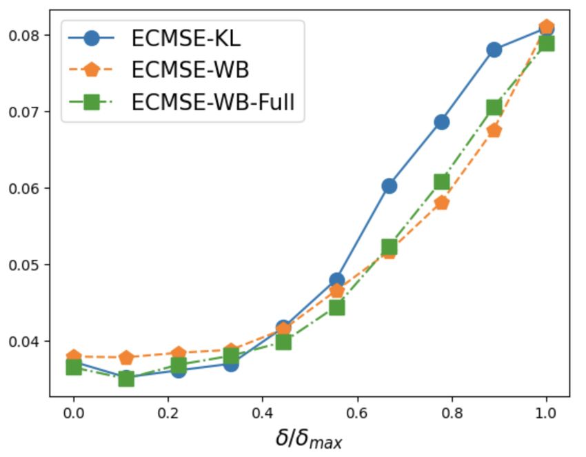
a training set consisting of T train periods, and the remaining T test = T − T train periods are used
as the testing set. We will be primarily concerned with the imputation of the training set.

                             Figure 1: Illustration of panel with missing data

This figure illustrates panel data D with missing entries in black. The observed components of Zt are denoted by
Xt , and the unobserved components of Zt are denoted by Yt .

      In this paper, we pursue the Bayesian approach: we assume that the vector θ ∈ Rn is unknown,
and is treated as a Bayesian parameter with a prior distribution π0 ; we also treat (Yt )t∈[T ] as
Bayesian parameters with appropriate priors. Based on the data set with missing entries D, our
strategy relies on computing the distribution of (Yt )t∈[T ] conditional on the data set D, and then
generate multiple imputations of (Yt )t∈[T ] by sampling from this distribution. To compute the
posterior of (Yt )t∈[T ] |D, we first need to calculate a posterior distribution of the unknown mean
vector θ conditional on D, and then the distribution of (Yt )t∈[T ] |D is obtained by marginalizing out
θ from the distribution of (Yt )t∈[T ] |(θ, D).
      We endeavor in this paper to explore a novel approach to generate multiply-imputed version of
the data set. We make the following assumptions.

Assumption 3.1 (Observability). We observe at least one value for each row in the training section
of D.

Assumption 3.2 (Ignorability). The missing pattern satisfies the ignorability assumption (Little
and Rubin, 2002), namely, the probability of (Mt )i = 1 ∀i ∈ [n] ∀t ∈ [T ] does not depend on (Yt )t∈[T ]
or θ, conditional on (Xt )t∈[T ] .

Assumption 3.3 (Bayesian conjugacy). The noise εt ∀t ∈ [T ] in the latent generative model (1)
is independently and identically distributed as Nn (0, Ω), where Ω ∈ Sn++ is a known covariance
matrix. The prior π0 is either a non-informative flat prior or Gaussian with mean vector µ0 ∈ Rn
and covariance matrix Σ0 ∈ Sn++ . The priors on Yt conditional on θ are independent across t, and
the conditional distribution is Gaussian Ndim(Yt ) (θYt , ΩYt ), where θYt = PMt (θ), and ΩYt is obtained
by applying the projection operator PMt on Ω.5
  5                                                                    >
      Using the construction of PMt in Footnote 4, we have ΩYt = PMt ΩPMt
                                                                          . Likewise for ΩXt . The latent generative

                                                          8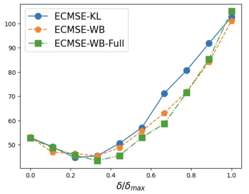
Figure 2: Illustration of workflow

This figures illustrates the workflow of our framework. The Bias-Variance Multiple Imputation (BVMI) framework
(contained in dashed box) receives a data set with missing values as an input, and generates multiple data sets
as outputs. The posterior generator (G) can exploit time dependency, while the consensus mechanism (C) is bias-
variance targeted.

    Following our discussion on the look-ahead bias, we can observe that the distribution of θ|D may
carry look-ahead bias originating from the testing portion of D, and this look-ahead bias will be
internalize into the look-ahead bias of (Yt )t∈[T train ] |D. To mitigate this negative effect, it is crucial
to re-calibrate the distribution of θ|D to reduce the look-ahead bias on the posterior distribution of
the mean parameter θ, with the hope that this mitigation will be spilt-over to a similar mitigation of
the look-ahead bias on the imputation of (Yt )t∈[T train ] . Our BVMI framework pictured in Figure 2
is designed to mitigate the look-ahead bias by implementing there modules:

 (G) The posterior Generator
 (C) The C onsensus mechanism
 (S) The multiple imputation S ampler

    For the rest of this section, we will elaborate on the generator (G) in Subsection 3.1, and we
detail the sampler (S) in Subsection 3.2. The construction of the consensus mechanism (C) is more
technical, and thus the full details on (C) will be provided in subsequent sections.

3.1     Posterior Generator
We now discuss in more detail how to generate multiple posterior distributions by taking into
account the time-dimension of the data set. To this end, we fix the desired number of posterior
distributions to K, (2 ≤ K ≤ T test +1). Moreover, we assign the integer values T1 , . . . , TK satisfying

                                         T train = T1 < T2 < . . . < TK = T
model (1) implies that the likelihood of Xt conditional on (θ, Yt ) is Gaussian Ndim(Xt ) θXt +ΩXt Yt Ω−1 Yt (Yt −θYt ), ΩXt −
ΩXt Yt Ω−1                            ⊥                               dim(Yt )×dim(Xt )

        Yt Ω Yt Xt  , where θ X t = PM  t
                                          (θ), the matrix ΩYt X t ∈ R                   is the covariance matrix  between Yt
and Xt induced by Ω, similarly for ΩXt Yt .

                                                              9
to indicate the amount of data that is synthesized in each posterior. The data set truncated to
time Tk is denoted as Dk = {(Xt , Mt ), t ∈ [Tk ]}, note that D1 coincides with the training data set
while DK coincides with the whole data set D. By construction, the sets Dk inherits a hierarchy in
terms of time: for any k < k 0 , the data set Dk is part of Dk0 , and thus Dk0 contains at least as much
of information as Dk . The k-th posterior for θ is formulated conditional on Dk . Under standard
regularity conditions, the posterior πk can be computed from the prior distribution π0 using the
Bayes’ theorem (Schervish, 1995, Theorem 1.31) as
dπk f (Dk |θ)
(θ|Dk ) = R , (2)
dπ0 Rn f (Dk |ϑ)π0 (dϑ)
where dπk /dπ0 represents the Radon-Nikodym derivative of πk with respect to π0 , and f (Dk |θ) is
the conditional density representing the likelihood of observing Dk given the parameter θ. Under
the generative model (1), and Assumption 3.2, we have
f (Dk |θ) = fX (Xt )t∈[Tk ] |θ ×fM (Mt )t∈[Tk ] |(Xt )t∈[Tk ] , θ = fX (Xt )t∈[Tk ] |θ ×f˜M (Mt )t∈[Tk ] |(Xt )t∈[Tk ]
for some appropriate (conditional) likelihood functions fX , fM and f˜M . In this case, the terms
involving (Mt )t∈[Tk ] in both the numerator and denominator of equation (2) cancel each other out,
hence (2) can be simplified to
dπk fX (Xt )t∈[Tk ] |θ
(θ|Dk ) = R ,
Rn fX (Xt )t∈[Tk ] |ϑ π0 (dϑ)
dπ0
Under Assumption 3.3, the posterior distribution πk can be computed more conveniently. As-
sumption 3.3 implies that conditioning on θ, the latent variables Zt and Zt0 are i.i.d. following a
Gaussian distribution with mean θ and covariance matrix Ω for any t, t0 . Because the operator PM
⊥
t
is an affine transformation (see Footnote 4), Theorem 2.16 in Fang, Kotz, and Ng (1990) asserts
that Xt |θ is Gaussian with mean θXt and covariance matrix ΩXt . In this case, the posterior πk can
be computed as Q
dπk t∈[Tk ] Ndim(Xt ) (Xt |θXt , ΩXt )
(θ|Dk ) = R Q ,
dπ0 Rn t∈[Tk ] Ndim(Xt ) (Xt |ϑXt , ΩXt )π0 (dϑ)
where Ndim(Xt ) ( · |θXt , ΩXt ) is the probability density function of the Gaussian distribution Ndim(Xt ) (θXt , ΩXt ).
Because π0 is either flat or Gaussian by Assumption 3.3, the Bayes’ theorem asserts that the poste-
rior πk also admits a density (with respect to the Lebesgue measure on Rn ). This density (we first
take the case that π0 is Gaussian for illustration) evaluated at any point θ ∈ Rn is proportional to
Y
Nn (θ|µ0 , Σ0 ) Ndim(Xt ) (Xt |θXt , ΩXt )
t∈[Tk ]
Y
1 > −1 1 > −1
∝ exp − (θ − µ0 ) Σ0 (θ − µ0 ) exp − (θXt − Xt ) ΩXt (θXt − Xt ) .
2 2
t∈[Tk ]
10By expanding the exponential terms and completing the squares, the posterior distribution θ|Dk is
then governed by πk ∼ Nn (µk , Σk ) with
−1
X X
Σk = Σ−1
0 +
⊥ −1
(PM t
) (Ω−1
Xt )
, µk = Σk Σ−1
0 µ0 +
⊥ −1
(PM t
) (Ω−1 ⊥ −1
Xt ) (PMt ) (Xt ) ,
t∈[Tk ] t∈[Tk ]
(3)
where ⊥ )−1
(PM is the inverse map of PM⊥ obtained by filling entries with zeros6 . An elementary
t t
linear algebra argument asserts that Ω−1
Xt is positive definite, and hence ⊥ )−1 (Ω−1 )
(PM t Xt is positive
semidefinite. The matrix inversion that defines Σk is thus well-defined thanks to the positive defi-
niteness of Σ0 in Assumption 3.3. Alternatively, in Assumption 3.3 if we impose a flat uninformative
prior on θ, then the posterior distribution of θ|Dk is still Gaussian with πk ∼ Nn (µk , Σk ) where
−1
X X
Σk = ⊥ −1
(PM t
) (Ω−1
Xt )
, µk = Σk ⊥ −1
(PM t
) (Ω−1 ⊥ −1
Xt ) (PMt ) (Xt ) .
(4)
t∈[Tk ] t∈[Tk ]
The following lemma ensures us that the covariance Σk is positive definite.
Lemma 3.4. Under Assumption 3.1, the posterior covariance (4) is positive definite.
The product of the posterior generator module (G) is K elementary posteriors {πk }k∈[K] , where
πk is the posterior of θ|Dk . For any k < k 0 , the definition of the set Dk and Dk0 implies that
the posterior πk0 carries at least as much of look-ahead bias as the posterior πk . The collection of
posteriors {πk } is transmitted to the consensus mechanism (C) to form an aggregated posterior π ?
that strikes a balance between the variance and the look-ahead-bias. The aggregated posterior π ?
is injected to the sampler module (S), which we now study.
3.2 Multiple Imputation Sampler
A natural strategy to impute the missing values depends on recovering the (joint) posterior distri-
bution of (Yt )t∈[T ] conditional on the observed data D. Fortunately, if the noise t are mutually
independent, and the priors on Yt are mutually independent given θ, it suffices to consider the
posterior distribution of Yt for any given t. Using the law of conditional probability and leveraging
the availability of the aggregated posterior π ? , we have for any measurable set Y ⊆ Rn
Z
P(Yt ∈ Y|D) = P(Yt ∈ Y|θ, D)π ? (dθ)
Rn
Z
= P(Yt ∈ Y|θ, Xt , Mt )π ? (dθ), (5a)
Rn
where the last equality holds thanks to the independence between Yt and any (Xt0 , Mt0 ) for t0 6= t
conditional on (θ, Xt , Mt ). Evaluating the posterior distribution for Yt |D thus entails a multi-
) (Ω−1 Xt }, where k · k0 is
(Ω̃) = Ω−1
6 ⊥ −1 n×n ⊥
This inverse map can be defined as (PM t Xt ) = arg min{kΩ̃k0 : Ω̃ ∈ R , PM t
⊥ −1
a sparsity inducing norm. Similarly for (PMt ) (Xt ).
11dimensional integration, which is in general computationally intractable.
Under Assumption 3.3, Zt conditional on θ is Gaussian Nn (θ, Ω). Because Zt is decomposed
into Xt and Yt , the distribution of Yt conditional on θ and (Xt , Mt ) is thus Gaussian (Cambanis,
Huang, and Simons, 1981, Corollary 5). More specifically,
Yt |θ, Xt , Mt ∼ Ndim(Yt ) θYt + ΩYt Xt Ω−1 −1
Xt (Xt − θXt ), ΩYt − ΩYt Xt ΩXt ΩXt Yt , (5b)
⊥ (θ), while Ω
where θXt = PMt (θ), θYt = PM t Xt and ΩYt are obtained by applying the projection
⊥ on Ω. The matrix Ω
operators PMt and PM dim(Yt )×dim(Xt ) is the covariance matrix between
t Yt Xt ∈ R
Yt and Xt induced by Ω. Notice that by the definitions of the projection operators, θXt and θYt
are affine transformations of θ. As a consequence, the mean of Y |θ, Xt , Mt is an affine function of
θ, while its covariance matrix is independent of θ. The posterior formula (5a) coupled with the
structural form (5b) indicate that the distribution of Yt |D coincide with the distribution of the
random vector ξt ∈ Rdim(Yt ) dictated by
ξt = At θ + bt + ηt , θ ∼ π?, ηt ∼ Ndim(Yt ) (0, St ), θ ⊥⊥ ηt , (6)
for some appropriate parameters At , bt and St that are designed to match the mean vector and
the covariance matrix of the Gaussian distribution in (5b). More specifically, we have At θ =
θYt −ΩYt Xt Ω−1 −1 −1
Xt θXt , bt = ΩYt Xt ΩXt Xt , St = ΩYt −ΩYt Xt ΩXt ΩXt Yt . Algorithm 1 details the procedure
for missing value imputation using the model (6).
The variability in the sampling of ξt using (6) comes from two sources: that of sampling θ
from π ? and that of sampling ηt from Ndim(Yt ) (0, St ). As we have seen from Section 3.1 (e.g.,
equations (3) and (4)), the posterior covariance of θ is inverse-proportional to the time-dimension
of the data set, and therefore the variability due to π ? is likely to be overwhelmed by the variability
due to ηt unless T is small. To fully exhibit the potential of the aggregated posterior π ? for bias
and variance trade-off, especially when validating our proposed method in numerical experiments,
we choose to eliminate the idiosyncratic noise ηt , namely, the missing values are imputed by its
conditional expectation given θ, which is depicted in Algorithm 2.
Algorithm 1 Fully Bayesian Imputation
Input: aggregated posterior π ? , data set D = {(Xt , Mt ) : t ∈ [T ]}, covariance
matrix Ω
Sample θ from π ?
for t = 1, . . . , T do
Compute At , bt , St for model (6) dependent on (Xt , Mt , Ω)
Sample ηt from Ndim(Yt ) (0, St )
Impute Yt by At θ + bt + ηt
end for
Output: An imputed data set
12Algorithm 2 Conditional Expectation Bayesian Imputation
Input: aggregated posterior π ? , data set D = {(Xt , Mt ) : t ∈ [T ]}, covariance
matrix Ω
Sample θ from π ?
for t = 1, . . . , T do
Compute At , bt for model (6) dependent on (Xt , Mt , Ω)
Impute Yt by At θ + bt
end for
Output: An imputed data set
4 Bias-Variance Targeted Consensus Mechanism
We devote this section to provide the general technical details on the construction of the consensus
mechanism module (C) in our BVMI framework. Conceptually, the consensus mechanism module
receives K posteriors {πk }k∈[K] from the posterior generator module (G), then synthesizes a unique
posterior π ? and transmits π ? to the sampler module (S). We first provide a formal definition of a
consensus mechanism.
Definition 4.1 (Consensus mechanism). Fix an integer K ≥ 2. A consensus mechanism Cλ :
MK → M parametrized by λ outputs a unifying posterior π ? for any collection of K elementary
posteriors {πk }.
We assume that the parameter λ is finite dimensional, and the set of all feasible parameters is
denoted by ∆K , which is a nonempty finite dimensional set. The space of all possible consensus
mechanism induced by ∆K is represented by C , {Cλ : λ ∈ ∆K }. For a given set of posteriors {πk },
we need to identify the optimal consensus mechanism Cλ? ∈ C in the sense that the aggregated
posterior π ? = Cλ? ({πk }) achieves certain optimality criteria. In this paper, the optimality criteria
of π ? is determined based on the notion of bias-variance trade-off, which is ubiquitously used in
(Bayesian) statistics. The first step towards this goal entails quantifying the bias of an aggregated
posterior π ? .
Definition 4.2 ((`, µ, δ)-bias tolerable posterior). Fix a penalization function ` : Rn → R, an
anchored mean µ ∈ Rn and a tolerance δ ∈ R+ . A posterior π ? is said to be (`, µ, δ)-bias tolerable
if `(Eπ? [θ] − µ) ≤ δ.
If ` is the Euclidean norm and the anchored mean is set to θtrue , then we recover the standard
measure of bias in the literature with the (subjective) posterior distribution in place of the (objec-
tive) frequentist population distribution, and a posterior π ? is unbiased if it is (k · k2 , θtrue , 0)-bias
tolerable.
Definition 4.2 provides a wide spectrum of options to measure the bias of the aggregated pos-
terior. Most importantly, we can flexibly choose a suitable value for the anchored mean µ for our
purpose of mitigating look-ahead bias. The tolerance parameter δ indicates how much of look-ahead
13bias is accepted in the aggregated posterior π ? . If δ = 0, then we are aiming for an aggregated
posterior distribution that has the exact mean vector µ. The generality of Definition 4.2 also allows
us to choose the penalization function. Throughout this paper, we will focus on the penalization
function of the form
`Z (µ) = sup z > µ (7)
z∈Z
parametrized by some nonempty, compact set Z ⊆ Rn . The functional form (7) enables us to model
diverse bias penalization effects as demonstrated in the following example.
Example 4.3 (Forms of `Z ). (i) If Z = {z ∈ Rn : kzk2 ≤ 1} is the Euclidean ball, then
`Z (µ) = kµk2 . This 2-norm penalization coincides with the canonical bias measurement
in the literature.
(ii) If Z is a convex polyhedron Z = {z ∈ Rn : Az ≤ b} for some matrix A and vector b of
appropriate dimensions, then `Z coincides with the support function of Z.
(iii) If Z = {1n }, then `Z is an upward bias penalization under the 1/n-uniform portfolio. The
1/n-uniform portfolio has been shown to be a robust portfolio (DeMiguel, Garlappi, and Uppal,
2007).
Next, we discuss the variance properties of the aggregated posterior. Let CovCλ ({πk }) [θ] ∈ Rn×n
be the covariance matrix of θ under the posterior distribution Cλ ({πk }). We consider the following
minimal variance criterion which is computed based on taking the sum of the diagonal entries.
Definition 4.4 (Minimal variance posterior). For a fixed input {πk }, the aggregated posterior π ?
obtained by π ? = Cλ? ({πk }) for an Cλ? ∈ C has minimal variance if
Tr(Covπ? [θ]) ≤ Tr(CovCλ ({πk }) [θ]) ∀Cλ ∈ C.
We are now ready to define our notion of optimal consensus mechanism.
Definition 4.5 (Optimal consensus mechanism). Fix an input {πk }. The consensus mechanism
Cλ? ∈ C is optimal for {πk } if the aggregated posterior π ? = Cλ? ({πk }) is (`, µ, δ)-bias tolerable and
has minimal variance.
Intuitively, the optimal consensus mechanism for the set of elementary posteriors {πk } is chosen
so as to generate an aggregated posterior π ? that has low variance and acceptable level of bias.
Moreover, because the ultimate goal of the consensus mechanism is to mitigate the look-ahead
bias, it is imperative to choose the anchored mean µ in an appropriate manner. As the posterior π1
obtained by conditioning on the training set D1 = {(Xt , Mt ) : t ∈ T train } carries the least amount
of look-ahead bias, it is reasonable to consider the discrepancy between the mean of the aggregated
posterior π ? and that of π1 as a proxy for the true bias. The optimal consensus mechanism can be
14constructed from λ? ∈ ∆K that solves the following consensus optimization problem
min Tr(CovCλ ({πk }) [θ])
s. t. λ ∈ ∆K (8)
`Z (ECλ ({πk }) [θ] − µ1 ) ≤ δ
for some set Z. Notice that problem (8) shares significant resemblance with the Markowitz’s
problem: the objective function of (8) minimizes a variance proxy, while the constraint of (8)
involves the expectation parameters.
So far, we have not yet specified how the mechanism Cλ depends on the parameters λ. In
its most general form, Cλ may depends nonlinearly on λ, and in this case, problem (8) can be
intractable. It behooves us to simplify this dependence by imposing certain assumptions on ∆K
and on the relationship between λ and Cλ . Towards this end, we assume for the rest of this paper
PK
that ∆K = {λ ∈ RK + : k=1 λk = 1}, a (K − 1)-dimensional simplex. Furthermore, Cλ depends
explicitly on λ through the following variational form
X
Cλ ({πk }) = arg min λk ϕ(π, πk ), (9)
π∈M
k∈[K]
where ϕ represents a measure of dissimilarity in the space of probability measures. If λ is a vector of
1/K, then C1/K 1 ({πk }) is the (potentially asymmetric) barycenter of {πk } under ϕ. The parameter
vector λ can now be thought of as the vector of weights corresponding to the set of posteriors {πk },
and as a consequence, the mechanism Cλ outputs the weighted barycenter of {πk }.
It is important to emphasize on the sharp distinction between our consensus optimization prob-
lem (8) and the existing literature on barycenters. While the existing literature typically focuses on
studying the barycenter for a fixed parameter λ, problem (8) searches for the best value of λ that
meets our optimality criteria. Put differently, one can also view problem (8) as a search problem
for the best reweighting scheme of {πk } so that their barycenter has minimal variance while being
bias tolerable.
The properties of the aggregation mechanism depends fundamentally on the choice of ϕ, and in
what follows we explore three choices of ϕ that are analytically tractable. In Section 5, we explore
the mechanism using the forward Kullback-Leibler divergence, and in Section 6, we examine the
mechanism under the type-2 Wasserstein distance. We will show that in these two cases, the
optimal consensus problem (8) is a convex optimization problem under specific assumptions. In
Section 7, we study the mechanism under the backward Kullback-Leibler divergence, and reveal
that the resulting consensus problem is non-convex.
5 Optimal Forward Kullback-Leibler Consensus Mechanism
In this section, we will measure the dissimilarity between distributions using the Kullback-Leibler
(KL) divergence. The KL divergence is formally defined as follows.
15Definition 5.1 (Kullback-Leibler divergence). Given two probability measures ν1 and ν2 with ν1
being absolutely continuous with respect to ν2 , the Kullback-Leibler (KL) divergence from ν1 to ν2
is defined as KL(ν1 k ν2 ) , Eν1 [log(dν1 /dν2 )], where dν1 /dν2 is the Radon-Nikodym derivative of
ν1 with respect to ν2 .
It is well-known that the KL divergence is non-negative, and it vanishes to zero if and only if
ν1 coincides with ν2 . The KL divergence, on the other hand, is not a distance: it even fails to
be symmetric, and in general we have KL(ν1 k ν2 ) 6= KL(ν2 k ν1 ). The KL divergence is also
a fundamental tools in statistics, information theory (Cover and Thomas, 2012) and information
geometry (Amari, 2016).
Under Assumption 3.3, the posteriors πk are Gaussian, hence, to compute the aggregated pos-
terior Cλ (πk ), we often need to evaluate the KL divergence from, or to, a Gaussian distribution.
Fortunately, when measuring the dissimilarity between two Gaussian distributions, the KL diver-
gence admits a closed-form expression.
Lemma 5.2 (Kullback-Leibler divergence between Gaussian distributions). For any (µi , Σi ), (µj , Σj ) ∈
Rn × Sn++ , we have
KL Nn (µi , Σi ) k Nn (µj , Σj ) , (µj − µi )> Σ−1 −1
− log det(Σi Σ−1
j (µj − µi ) + Tr Σi Σj j ) − n.
In this section we use ϕ as the forward KL-divergence to aggregate the posteriors; more specif-
ically, for any two probability distributions ν1 and ν2 , we use ϕ(ν1 , ν2 ) = KL(ν1 k ν2 ). Note that
this choice of ϕ places the posteriors πk as the second argument in the divergence. We use CλF to
denote the consensus mechanism induced by the forward KL-divergence, and CλF is formally defined
as follows.
Definition 5.3 (Forward KL consensus mechanisms). A mechanism CλF with weight λ is called a
forward KL consensus mechanism if for any collection of posterior distributions {πk }, we have
X
CλF ({πk }) = arg min λk KL(π k πk ). (10)
π∈M
k∈[K]
The KL barycenter of the form (10) is widely used to fuse distributions and aggregate infor-
mation, and it has witnessed many successful applications in machine learning (Claici, Yurochkin,
Ghosh, and Solomon, 2020; Da, Li, Zhu, Fan, and Fu, 2020; Li, Hlawatsch, and Djurić, 2019). The
set of forward KL mechanisms parametrized by the simplex ∆K is denoted by CF , {CλF : λ ∈ ∆K }.
For a given input {πk } and weight λ ∈ ∆K , computing CλF ({πk }) requires solving an infinite di-
mensional optimization problem. Fortunately, when the posteriors πk are Gaussian under Assump-
tion 3.3, we can characterize CλF analytically thanks to the following proposition.
Proposition 5.4 (Closed form of the consensus (Battistelli, Chisci, Fantacci, Farina, and Graziano,
2013)). Suppose that πk ∼ N (µk , Σk ) with Σk 0 for any k ∈ [K]. For any λ ∈ ∆K , we have
16CλF ({πk }) = N (b
µ, Σ)
b with
X X X
λk Σ−1 −1
λk Σ−1 ∈ Rn , λk Σ−1 −1
∈ Sn++ .
µ
b=( k ) k µ k Σ
b=(
k ) (11)
k∈[K] k∈[K] k∈[K]
Next, we discuss the tractability of the bias constraint under the forward KL consensus mech-
anism. For a given collection of posterior distributions {πk }, define the following set
n o
ΛF`Z ,δ ({πk }) = λ ∈ ∆K : `Z (EC F ({πk }) [θ] − µ1 ) ≤ δ
λ
that contains all the parameters λ ∈ ∆K for which the forward KL mechanism CλF satisfies the
(`Z , µ1 , δ)-bias requirement. Unfortunately, despite the analytical expression for the aggregated
posterior in Proposition 5.4, it remains difficult to characterize the set ΛF`Z ,δ ({πk }) in its most
general form. This difficulty can be alleviated if we impose additional assumptions on {πk } and
the set Z.
Proposition 5.5 ((`Z , µ1 , δ)-bias forward KL mechanisms). Suppose that there exists an orthogonal
matrix V ∈ Rn×n and a collection of diagonal matrices Dk = diag(dk ) ∈ Sn++ for k ∈ [K] such that
Σk = V Dk V > 0 and πk ∼ N (µk , Σk ) for all k ∈ [K]. If Z = {z ∈ Rn : kV > zk1 ≤ 1}, then
( P )
k∈[K] ckj λk
ΛF`Z ,δ ({πk }) = λ ∈ ∆K : −δ ≤ P −1 − vj> µ1 ≤δ ∀j ∈ [n] , (12)
k∈[K] dkj λk
where dkj is the j-th component of the vector dk , V = [v1 , . . . , vn ], and
vj> µk
ckj = ∀(k, j) ∈ [K] × [n].
dkj
We are now ready to state the main result of this section, which provides a reformulation of
problem (8) under conditions of Proposition 5.5.
Theorem 5.6 (Optimal forward KL mechanism). Suppose that there exists an orthogonal matrix
V ∈ Rn×n and a collection of diagonal matrices Dk = diag(dk ) ∈ Sn++ for k ∈ [K] such that Σk =
V Dk V > 0 and πk ∼ N (µk , Σk ) for all k ∈ [K], and suppose that Z = {z ∈ Rn : kV > zk1 ≤ 1}.
Let λ? be the optimal solution in the variable λ of the following second-order cone optimization
17problem X
min γj
j∈[n]
s. t. λ ∈ ∆K , γ ∈ Rn+
X X
ckj λk ≤ (δ + vj> µ1 ) d−1
kj λk
(13)
k∈[K] k∈[K]
X X
ckj λk ≥ (vj> µ1 − δ) d−1
kj λk
∀j ∈ [n],
k∈[K]
" # k∈[K]
2
P −1
P −1
≤ k∈[K] dkj λk + γj
k∈[K] dkj λk − γj
2
where dkj is the j-th component of the vector dk , V = [v1 , . . . , vn ], and
vj> µk
ckj = ∀(k, j) ∈ [K] × [n].
dkj
Then CλF? is the optimal consensus mechanism in CF , that is, CλF? is (`Z , µ1 , δ)-bias tolerable and
has minimal variance.
Problem (13) is a tractable convex optimization problem, and it can be readily solved using
off-the-shelf conic solvers such as MOSEK (MOSEK ApS, 2019). Note that the tractability of the
reformulation (13) depends crucially on the assumption that the covariance matrices Σk are simul-
taneously diagonalizable. However, this assumption is rarely satisfied in reality. We now discuss a
pre-processing step which projects all the covariance matrices Σk onto a common eigenbasis. To
this end, for a given orthogonal matrix V ∈ Rn×n , we define the following subspace of Gaussian
distributions
NV , π ∈ M : ∃(µ, d) ∈ Rn × Rn++ , Σ = V diag(d)V > , π ∼ N (µ, Σ)
that contains all nondegenerate Gaussian distributions whose covariance matrix is diagonalizable
with respect to V . Given any posterior πk ∼ N (µk , Σk ), we add a pre-processing step to create
πk0 ∼ N (µk , Σ0k ) with Σ0k being diagonalizable with the orthogonal matrix V based on the following
lemma.
Lemma 5.7 (Projection on NV ). Let V be an orthogonal matrix. Suppose that πk ∼ N (µk , Σk )
for some µk ∈ Rn and Σk ∈ Sn++ , then the following holds:
(i) Let dk ∈ Rn++ be such that (dk )j = vj> Σk vj for j ∈ [n]. Then the distribution πk0 ∼ N (µk , Σ0k )
with Σ0k = V diag(dk )V > is the optimal solution of
min KL(πk k πk0 ).
πk0 ∈NV
(ii) Let dk ∈ Rn++ be such that (dk )j = [V > (Σk )−1 V ]jj for j ∈ [n]. Then the distribution
18πk0 ∼ N (µk , Σ0k ) with Σ0k = V diag(dk )V > is the optimal solution of
min KL(πk0 k πk ).
πk0 ∈NV
6 Optimal Wasserstein Consensus Mechanism
In this section, we will measure the dissimilarity between distributions using the Wasserstein type-2
distance.
Definition 6.1 (Wasserstein distance). Given two probability measures ν1 and ν2 , the type-2
Wasserstein distance between ν1 and ν2 is defined as
Z 1
2
W2 (ν1 , ν2 ) , min kθ1 − θ2 k22 γ(dθ1 , dθ2 ) ,
γ Rn ×Rn
where the minimization is taken over all couplings of ν1 and ν2 .
The type-2 Wasserstein distance W2 is non-negative and it vanishes only if ν1 = ν2 . Moreover,
W2 is symmetric and satisfies the triangle inequality. As a consequence, W2 represents a metric
on the space of probability measures (Villani, 2008, p. 94). The type-2 Wasserstein distance W2
is a fundamental tool in the theory of optimal transport, and its squared value can be interpreted
as the minimum cost of transporting the distribution ν1 to ν2 , in which the cost of moving a unit
probability mass is given by the squared Euclidean distance. The application of the Wasserstein
distance has also been extended to economics (Galichon, 2016), machine learning (Kuhn, Esfahani,
Nguyen, and Shafieezadeh-Abadeh, 2019) and statistics (Panaretos and Zemel, 2019).
As the posteriors πk are Gaussian underAssumption 3.3, we often need to evaluate the Wasser-
stein distance from a Gaussian distribution. Conveniently, the Wasserstein distance between two
Gaussian distribution can be written in an analytical form (Givens and Shortt, 1984).
Definition 6.2 (Wasserstein type-2 distance between Gaussian distributions). The Wasserstein
W2 distance between N (µ, Σ) and N (µ0 , Σ0 ) is given by
q
1 1 1
0 0
kµ − µ0 k22 + Tr Σ + Σ0 − 2 (Σ0 ) 2 Σ(Σ0 ) 2 2 .
W2 N (µ, Σ), N (µ , Σ ) =
In this section we use ϕ as the Wasserstein distance W2 to aggregate the posteriors. In more
details, for any two probability distributions ν1 and ν2 , we use ϕ(ν1 , ν2 ) = W2 (ν1 , ν2 ). We use CλW
to denote the consensus mechanism induced by the Wasserstein metric, and CλW is formally defined
as follows.
Definition 6.3 (Wasserstein consensus mechanisms). A mechanism CλW with weight λ is called a
Wasserstein consensus mechanism if for any collection of posterior distributions {πk } ∈ N K , we
have
X
CλW ({πk }) = arg min λk W2 (π, πk )2 . (14)
π∈N
k∈[K]
19You can also read


