Biological Network Inference with GRASP: A Bayesian Network Structure Learning Method Using Adaptive Sequential Monte Carlo

Biological Network Inference with GRASP: A
Bayesian Network Structure Learning Method Using
Adaptive Sequential Monte Carlo
Kaixian Yu
 Didi Chuxing
Zihan Cui
 Florida State University
Xin Sui
 Florida State University
Xing Qiu
 University of Rochester
Jinfeng Zhang (  jinfeng@stat.fsu.edu )
 Florida State University

Research Article

Keywords: Bayesian Network, Bayesian Network structure learning, sequential Monte Carlo, adaptive
sequential Monte Carlo, GRASP for BN structure learning.

Posted Date: January 21st, 2021

DOI: https://doi.org/10.21203/rs.3.rs-148701/v1

License:   This work is licensed under a Creative Commons Attribution 4.0 International License.
Read Full License

Biological network inference with GRASP: a
 Bayesian network structure learning
 method using adaptive sequential Monte Carlo
 Kaixian Yu1,*, Zihan Cui2, Xin Sui2, Xing Qiu3 and Jinfeng Zhang2,*
 1
 Didi Chuxing, Beijing, China
 2
 Department of Statistics, Florida State University, Tallahassee, FL, 32304
3
 Department of Biostatistics and Computational Biology, University of Rochester, Rochester, NY
 14624, USA
 *
 Correspondence: jinfeng@stat.fsu.edu, kaixiany@gmail.com

Abstract:
Bayesian networks (BNs) provide a probabilistic, graphical framework for modeling high-
dimensional joint distributions with complex correlation structures. BNs have wide applications
in many disciplines, including biology, social science, finance and biomedical science. Despite
extensive studies in the past, network structure learning from data is still a challenging open
question in BN research. In this study, we present a sequential Monte Carlo (SMC)-based three-
stage approach, GRowth-based Approach with Staged Pruning (GRASP). A double filtering
strategy was first used for discovering the overall skeleton of the target BN. To search for the
optimal network structures we designed an adaptive SMC (adSMC) algorithm to increase the
quality and diversity of sampled networks which were further improved by a third stage to
reclaim edges missed in the skeleton discovery step. GRASP gave very satisfactory results when
tested on benchmark networks. Finally, BN structure learning using multiple types of genomics
data illustrates GRASP’s potential in discovering novel biological relationships in integrative
genomic studies.

Keywords: Bayesian Network, Bayesian Network structure learning, sequential Monte Carlo,
adaptive sequential Monte Carlo, GRASP for BN structure learning.

Introduction
 A Bayesian network (BN) is a graphical representation of the joint probability distribution of a
set of variables (called nodes in the graph). BNs have been widely used in various fields, such as
computational biology (Friedman, Linial, Nachman and Pe'er 2000, Raval, Ghahramani and Wild
2002, Vignes, et al. 2011), document classification (Denoyer and Gallinari 2004), and decision
support system (Kristensen and Rasmussen 2002). BN encodes conditional dependencies and
independencies (CDIs) among variables into a directed acyclic graph (DAG). And this DAG is called
the structures of a BN. When the structure of a BN is given, the parameters that quantify the CDIs
can be estimated from the observed data. If neither the parameters nor structures are given,
they can be inferred from observed data. In this study, we will be focusing on the structure
estimation of a BN and its application in learning real biological networks using heterogeneous
genomics data.
 The technical difficulties of structure learning are mainly due to the super-exponential
cardinality of the DAG spaces, which are also quite rugged for most commonly used score
functions. Estimating the structure exactly is an NP-hard problem (Cooper 1990, Koller and
Friedman 2009). There have been many inexact and heuristic methods proposed in the past two
decades. The strategy of these methods can be classified mainly into three categories: constraint-
based, score-based, and hybrid, which combines both constraint-based and score-based
approaches.
 A constraint-based method utilizes the conditional dependency test to identify the conditional
dependencies and independencies among all nodes (Campos 1998, de Campos and Huete 2000,
Margaritis 2003, Tsamardinos, Aliferis and Statnikov 2003, Yaramakala and Margaritis 2005,
Aliferis, Statnikov, Tsamardinos, Mani and Koutsoukos 2010). A major disadvantage of such a
method is that a large number of tests have to be conducted; therefore, an appropriate method
to adjust the p-values obtained from all the tests should be applied. The fact that not all the tests

are mutually independent further complicates the p-values adjustment. Another issue is that the
goodness-of-fit of the obtained network is usually not considered in such approach; therefore,
the estimated BN may not fit the observed data well.
 A score-based method uses a score function to evaluate the structures of BNs on training data
(Larrañaga, Poza, Yurramendi, Murga and Kuijpers 1996, Friedman, Nachman and Peér 1999,
Gámez, Mateo and Puerta 2011). A searching algorithm is employed to search the best BN (with
the highest score) with respect to certain score function. Various Bayesian and non-Bayesian
score functions have been proposed in the past. As exact search is not feasible, over the past two
decades, various heuristic searching methods, such as Hill climbing, tabu search, and simulated
annealing were proposed to search for the optimal BN structures. The problem with score-based
method is that the searching space is often very large and complicated; therefore, the searching
algorithm either will take too much time to find the optimum or be trapped in local optima. Many
efforts have been made to overcome this challenging issue, such as searching using an ordered
DAG space to reduce the searching space (Teyssier and Koller 2012). In the ordered DAG space,
the nodes are given an order such that edges will only be searched from higher order to lower
order. The practical issue is that determining the order and finding the optimal structure is
equally difficult. More recently, various penalty-based methods were proposed to estimate the
structures for Gaussian BN (GBN) (Fu and Zhou 2013, Huang, et al. 2013, Xiang and Kim 2013).
These methods have been shown to be quite efficient for GBN structure learning and are able to
handle structure learning and parameter estimation simultaneously; however, these methods
are quite restrictive: the joint distributions must approximately follow a multivariate Gaussian
distribution and dependencies among nodes are assumed to be linear.
 Hybrid methods which combine a constraint method and a score-based method were
proposed to combine the advantages of both methods (Tsamardinos, Brown and Aliferis 2006).
Such methods often contain two stages: first pruning the searching space by constraint-based
methods, then searching using a score function over the much smaller pruned space. In the
pruning stage, the goal is to identify the so-called skeleton of the network, which is the
undirected graph of the target DAG. Later in the second stage, the direction of each edge will be
determined by optimizing the score function. In a hybrid method, it is important that the first
stage identifies as many true undirected edges as possible, since only the identified undirected
edges will be considered in the second stage.
 In this study, we developed a novel BN structure learning method named GRASP (GRowth-
based Approach with Staged Pruning). It is a three-stage method: in stage one, we used a double
filtering method to discover a cover of the true skeleton. Unlike the traditional constraint
methods, which try to obtain the true skeleton exactly, our method only estimates a super set of
the undirected edges and it only conditions on at most one node other than the pair of nodes
being tested, which dramatically reduces the number of observations needed to make the test
results robust. In stage two, we designed an adaptive sequential Monte Carlo (adSMC) (Liu and
Chen 1998, Liu 2008) approach to search for a BN structure with optimal score based on
constructed skeleton. SMC has been successfully adopted to solve optimization problems in the
past (Grassberger 1997, Zhang and Liu 2002, Zhang, Lin, Chen, Liang and Liu 2007, Zhang, et al.
2009). Compared to most greedy searching methods, SMC is less likely to be trapped in local
optima. Another advantage of SMC is that it can be run in parallel for each SMC sample, making
it suitable for distributed or GPU-based implementations. To further increase the efficiency of

the sampling, an adaptive SMC strategy was used to generate higher scored networks. After
these two stages, we enhanced the traditional two-stage approach with a third stage which adds
possible missed edges back into the network using Random Order Hill Climbing (ROHC).

Methods and Data

GRASP: GRowth-based Approach with Staged Pruning
 GRASP is a three-stage algorithm for learning the structure of a BN. In the first (pruning)
stage, we designed a Double Filtering (DF) method to find the cover of the skeleton of the BN,
where the skeleton of a BN is defined as the BN structure after removing the direction of all the
edges, and the cover is defined as a superset of undirected edges containing all the edges of the
skeleton. In the second (structure searching) stage, we developed an adaptive sequential
Monte Carlo (adSMC) method to search the BN structure on the undirected network found in
the first stage based on Bayesian information criterion (BIC) score. To reclaim the potentially
missed edges, we designed a Random Ordered Hill Climbing (ROHC) method as the third stage.
First stage: Double Filtering (DF) method to infer the skeleton. The first stage, namely Double
Filtering (DF) method, contains two filtering processes. The first filtering was done by uncondi-
tioned tests, filtering out the nodes that are not ancestors or descendants of a given node .
The second filtering was built on conditioned tests, further filtering out the nodes that are not
direct neighbors (parents or children) of .
 Suppose we have nodes. For a given node , let ( ) be the set of nodes that have an
undirected edge with . The procedure of the DF method is as follows:
 1. First filtering: conduct an unconditioned dependency test for each pair of nodes ( and
 , ≠ ). We used mutual information (MI) test, which was also used by other BN
 structure learning methods (Campos 2006). Record the p-value of MI test as . If < ,
 update ( ) as ( ) ∪ { }. is the predefined significance level for the test. Sort
 each ( ) = { 1 , . . . , }, 1 , … , ∈ {1,2, … , } using their p-values, from smallest to
 largest to obtain ( ) = { ( 1) , … , ( ) }, where ( 1 ) ≤ ( 2 ) ≤, … , ( ) .
 2. Second filtering: update ( ) as follow:
 (a). For each node ( ) , = 1,2, … , , in ( ) , let ( , ( ) ) = ( ) ∩
 ( ( ) ) = { 1 , … , }, where 1 , … ∈ { 1 , … , } ∖ {( )}.
 (b). If ( , ( ) ) ≠ ∅, perform a conditional dependency test for and each in
 ( , ( ) ), given ( ) . If the p-value > , mark ∈ ( ) as removed.
 (c). If ( , ( ) ) = ∅, move on to ( +1) and start over from (a) until every node in
 ( ) is consumed.
 After (a)-(c), we can update ( ) from the first filtering to ( ) = { | ∈
 ( ) and not marked removed}, which is the final result of DF method for node .
 This DF method is applied on all nodes. The collection of ( ), = 1,2, . . . , gives us
 the skeleton of BN.

Second stage: structure searching. In the pruned space, we designed an adaptive sequential
Monte Carlo (adSMC) method to search the structure of the Bayesian network ( ( , )). In a
traditional sequential Monte Carlo, random variable ∈ is decomposed into( , , … , )
where ∈ and ∑ =1 = , and the decomposition is predefined and fixed throughout
the whole sampling procedure. One usually samples at first, then , and so on. However,
the sequence each variable is sampled (namely sampling sequence in this study) based on any
prior decomposition may not be the most efficient one. The optimal sampling sequence may
need to be decided dynamically. For example, when , , … , have been sampled for some
0 < < , the conditional distribution ( +1 | , , … , ) may have a small set of candi-
date decompositions (to satisfy the acyclic condition) which limits the diversity of the SMC sam-
ples. Therefore, we designed our sampling block conditioning on the current sampled struc-
ture 1 , 2 , … , −1 to increase the diversity and quality of obtained samples (see Figure S1 in
Supplementary Materials for an example).
 For each SMC sample, we start with all possible fully connected triplets (three nodes connected
by three undirected edges) discovered in the first stage. We sample one such triplet having the
least outside connection, e.g. the one having the least undirected edges connected to its nodes
(Figure 1A). These triplets are likely to be restricted to certain configuration by the sampled
structure; therefore, to sample them earlier allows more variety in their configurations. When all
fully connected triplets are sampled, partially connected triplets (two undirected edges among
three nodes) are considered (Figure 1B). Lastly, we consider pairs (the remaining undirected
edges, Figure 1C). For partially connected triplets and pairs, the configurations with the least
outside connections are sampled first.

Figure 1: Structure discovering procedure.

 The probabilities of possible configurations of triplets and pairs are proportional to their BIC
(Bayesian Information Criterion) score defined as = ln( ) ∙ − 2 ∙ ( ̂) , where 
represents sample size, represents number of parameters of the partial BN model, and ̂ =
 ( | ̂ , ) is the maximized value of the likelihood function of the model , with estimated
parameters, ˆ , from observed data . The probability is set to be 0 if certain configuration fails
to satisfy the acyclicity condition. In summary, for triplets (pairs), we calculate the BIC for all
possible configurations of this triplet (pair) and sample one configuration with probability
 
 exp ( ), if configuration i does not result in a loop
 (configuration ) ∝ { (1)
 0, if configuration i result in a loop
Where is temperature, controlling how greedy we want the searching to be.
 The main algorithm used in the second step is as follows.
 Step 1: Sample one fully connected triplet { , , } with the least outside connection;
 Choose a configuration between these three nodes with probability described in equation
 (1); Then remove the connection between , and from the skeleton.
 Step 2: Repeat step 1 until all fully connected triplets are sampled.
 Step 3: Sample one partially connected triplet { , , } with the least outside
 connection. Choose a configuration between these three nodes with probability described

in equation (1). Then remove the connection between , and (if applicable) from
 the skeleton.
 Step 4: Repeat step 3 until all partially connected triplets are sampled.
 Step 5: Sample one pair { , } with the least outside connection. Choose a configuration
 between them (either → or ← ) with probability described in equation (1). Then
 remove the connection between and from the skeleton.
 Step 6: Repeat step 5 until all pairs are sampled and no more unsampled edges in the
 skeleton.
 Since each SMC sample is generated independently, we can run our algorithm in parallel on
multiple CPUs/GPU cores to speed up the sampling process.

Third stage: reclaiming missed edges. We mentioned earlier that one disadvantage of the tra-
ditional two-stage method was that the edges missed in the first stage will never be recovered.
Therefore, in the third stage we designed a Random Order Hill Climbing (ROHC) method to
identify the possible missed edges and refine the network. The general idea is described as fol-
lows:
 1. Generate a permutation of 1,2, … , for each network sampled by adSMC in stage 2,
 suppose = 1 , … , is such a permutation.
 2. For every ∈ , iterate j from 1 through . If ← does not create loop and
 results in an increasing in BIC, then we add edge ← .
 3. Repeat (2) until there is no possible edge to add or the searching limit is reached.
 One could also view this stage as a further ascent to the local optima to ensure we achieve the
best possible BIC score.
 In general, generating more SMC samples gives a higher chance to reach the optimum.
However, more samples also require more computation time; therefore, a balance between
running time and sample sizes must be made. In most of our simulation study and practical
problems, we found that around 20,000 samples were often good enough for finding a network
with a satisfactory BIC score.

Performance evaluation
 To measure the effectiveness of edge screening methods, we employed the precision, recall
and f-score measurements. Precision is defined as TP/(TP+FP), recall is defined as TP/(TP+FN),
and f-score is the harmonic mean of precision and recall, 2(precision×recall)/(precision+recall),
where TP means true positive (number of true undirected edges identified), FP false positive
(number of non-edges identified as undirected edges), and FN false negative (number of
undirected edges not identified).
 In our study, recall measures the percentage of true edges (irrespective of their directions)
identified; therefore, it is the most important measurement in edge screening stage, since as we
discussed earlier, any missed edges in stage one may never be reclaimed in a traditional two
stage approach. Besides the recall, f-score is also important since it measures a balanced
performance in terms of both precision and recall. It is obvious that if we propose all possible

edges, we will always identify all true edges, but that will not do any pruning to the searching
space. Thus, a high f-score is desired for a decent edge screening strategy.
 We used Bayesian Information Criterion (BIC) as the score function in both second stage and
third stage. BIC has the score-equivalent property (Appendix definition 10), which can reduce the
searching space, since if we could find one network in the equivalent class, we found the true
network. And the consistency property of BIC score guarantees that the true network has the
highest score asymptotically.

Benchmark networks
 The networks used to generate simulated data (see Table 1) are from actual decision making
processes of a wide range of real applications including risk management, tech support, and
disease diagnosis. All networks are obtained from Bayesian Network Repository maintained by
M. Scutari http://www.bnlearn.com/bnrepository/.

 Table 1: Bayesian networks used in the simulation study.
 Name # of nodes # of edges # of parameters max in-degree
 Alarm 37 46 509 4
 Andes 223 338 1157 6
 Child 20 25 230 2
 Hailfinder 56 66 2656 4
 Hepar2 70 1236 1453 6
 Insurance 27 52 984 3
 Win95pts 76 112 574 7

 We randomly generated data with 1000, 2000, and 5000 observations, and we generated 10
datasets for each size of observations. All results reported in this section are based on averages
of 10 datasets. Observation size in this article refers to the number of data points, and shall not
be confused with number of sequential Monte Carlo samples. The datasets were generated using
R package bnlearn (Scutari 2009, Nagarajan, Scutari and Lèbre 2013).

Real Data
Flow cytometry dataset. In the flow cytometry dataset (Sachs, Perez, Pe'er, Lauffenburger and
Nolan 2005), there are 11 proteins and phospholipid components of the signaling network. The
original data was collected from 7466 cells, containing continuous variables. Sachs et al sug-
gested to get rid of the potential outliers by removing data that are 3 standard deviations away
from any attribute. Thus the data we are analyzing contains 6814 observations. We discretized
each variable into 3 categories, practically stands for high/medium/low, with each category
containing 33% of the data.
Genomics and Epigenomics data from the Cancer Genome Atlas (TCGA). We used several dif-
ferent types of data obtained from TCGA: RNA-seq, protein expression, DNA methylation, and
microRNA-seq, which have been used in our previous studies (Stewart, Luks, Roycik, Sang and
Zhang 2013, Li, et al. 2017, Shi, et al. 2017, Li, et al. 2020).

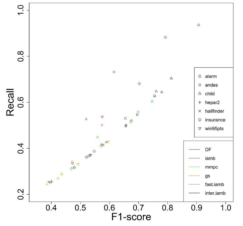
Results

Edge Screening
 The principal of the edge screening stage is pruning the searching space as much as possible
while the remaining edges in the pruned space still possess as many true edges as possible. We
compare our method to five other methods including max-min parent-child (mmpc)
(Tsamardinos, et al. 2006), grow-shrink (gs) (Margaritis 2003), incremental association (iamb)
(Tsamardinos, et al. 2003), fast iamb, and inter iamb (Yaramakala, et al. 2005). For all methods,
we fixed the significance level (α) to 0.01.
 The simulation study results (Figure 2 and Figure S2) showed that our double filtering (DF)
method was able to identify the most edges (highest recall) for each of the observation size we
tested. In some cases we observed that with even 1000 observations, our method achieved a
higher recall than the other methods using 5000 observations and the f-scores are still
comparable (e.g. Alarm, Hepar2 and etc.). For some networks (Child, Insurance), not only the
recalls were higher but also the f-scores were higher for DF. The results confirmed that DF
identifies true edges more accurately than other methods and it often requires fewer
observations. Higher recall is desired in the first stage (the edge screening stage) since any missed
edges will not be sampled in the second stage.

Figure 2: F1-score and recall of different methods with observation size 1000. One can see that
DF (the red points with different shapes) generally has higher recalls with higher or comparable
 F1-scores for the same network.

Effect of temperature. The temperature parameter in SMC has the same effect as that in
MCMC (Markov Chain Monte Carlo) simulations. A lower temperature will cause searching to
become greedier, and higher temperatures make it less greedy. When → 0 the searching pro-
cedure becomes a local greedy search. On the other hand, whenT → ∞ , the configuration is
sampled uniformly. The optimal temperature is usually a value in between. In this simulation
study, we fixed SMC sample size to 20,000, and rounds of ROHC to 5. The temperature was set
to between 10−7 and 10−1 , increased by 10-time each time (Figure S3). The performance is
shown in the relative scale (BIC of true network/BIC of the learned network), where higher ratio
means higher BIC score; thus, better network structure. Lower temperature in most cases gave
a lower score, as well as the higher temperature, consistent with what we would expect. Most
of the optimal scores happened around T = 0.001 or 0.01. We can also see that the optimal
temperature does not depend on the observation sizes, since the optimal temperatures are the
same across the 3 different observation sizes. Another observation we had was that the optimal
temperatures do not change much when the number of variables (nodes) changes. From figure
S3 we can see that for Andes (with 223 nodes) and child (20 nodes), the optimal temperature is
both around 0.01 and 0.001.
Effect of adaptive SMC. To show the improvement of using adaptive SMC, we compared the BICs
of 20,000 SMC samples between the adSMC and traditional SMC (Figure S4). In the traditional
SMC, we designed the sampling block in the order of fully connected triplets, partially connected
triplets and pairs, and started from least outside connected ones. Clearly, the adSMC generates
higher scored networks in general.

Effect of the edge reclaiming step. We discussed earlier that there could be some true edges
missed in the first stage due to the test power and limited data. Here we will show that Random
Order Hill Climbing (ROHC) indeed improves the learned BN structure in stage 2. We used alarm
and win95pts networks to illustrate the improvement made by ROHC (Figure S5). They both had
significance level cut-off of 0.01, temperature 0.001, and 20,000 SMC samples. As we can see,
the improvements were substantial, demonstrating that it is necessary to have the third stage
to further refine the learned network. However, one should notice that the complexity level of
ROHC is approximately ( 2 ); therefore, in a typical network with hundreds of nodes only 1 or
2 rounds of ROHC are affordable.

Performance on benchmark networks. We evaluated the overall performance of our method
and the general two stage methods (5 edge screening methods, gs, mmpc, iamb, fast.iamb, and
inter.iamb combined with 2 optimization methods, Hill climbing and tabu search) on 7 bench-
mark networks. The results are shown in Figure 3 and Figure S6 (Supplementary Material). For 3

different observation sizes, our method outperformed all the general two-stage methods on al-
most all benchmark networks except on the hepar2 network where all methods achieved simi-
lar scores, which are very close to the BIC of the true network.

 Figure 3: BIC scores of all methods on 7 benchmark networks with observation size 1000.
 GRASP has higher BIC scores for all the benchmark networks.

 Performance on the flow cytometry data. We first compared our method to the general 2-
stage methods and the CD method (Fu, et al. 2013) on the flow cytometry data. GRASP achieved
the highest BIC score (Figure 4), which is consistent with the simulation study.

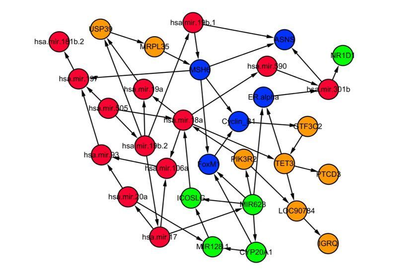
Figure 4: BIC scores for the flow cytometry data, comparing 12 methods, and GRASP has the
highest BIC score. The y-axis value is the ratio of the BIC score of the sampled network and the
 true network. It is possible that a sampled network has even higher BIC score than the true
 network, hence the value can be higher than 1.

 An integrative genomic study using TCGA data. An advantage of BN models is that they can
handle heterogeneous data well. In this section, we will test our method using a heterogeneous
genomics dataset from TCGA through learning network structures that may shed light on real
biological problems. In a previous study of ours (Stewart, et al. 2013), we have identified a long
non-coding RNA, LOC90784, which is strongly associated with breast cancer health disparity
between African American and Caucasian American breast cancer patients. However, literature
search resulted in no information about it since it had not been studied by any researchers in the
past. Using several different types of genomics data, we applied GRASP to perform an integrative
study to build a Bayesian network with different genomics features to shed some light on the
function of this transcript. We first used RNA-seq data to identify transcripts highly correlated
with LOC90784. This gave us 8 transcripts with absolute value of correlation coefficient greater
than 0.27. We then found other genomic features, including microRNAs, DNA methylations and
protein expressions that are highly correlated with these transcripts, which gave us 13 microRNAs,
5 DNA methylation regions (aggregated around genes) and 5 proteins. Using the samples with all
the above measurements, we inferred the BN structure for these genomics features as shown in

Figure 5. As a comparison, bnlearn, a R package for BN structure learning, gave a network without
LOC90784 (Supplementary material Figure S7). Figure 5 showed rather complex relationships
among all these genomic features. A thorough investigation of this network is beyond the scope
of this work. However, some literature search on the nodes around LOC90784 provided
interesting hypotheses, which could be followed up with experiments. Specifically, TET3, an
upstream gene, was found to inhibit TGF-β1-induced epithelial-mesenchymal transition in
ovarian cancer cells (Ye, et al. 2016). High frequency of PIK3R2 mutations in endometrial cancer
was found to be related to the regulation of protein stability of PTEN (Cheung, et al. 2011), which
is a well-known cancer related gene. There are not a lot of published studies on IRGQ. From the
Human Protein Atlas database (https://www.proteinatlas.org/ENSG00000167378-
IRGQ/pathology) we found that this gene is a prognostic biomarker and significant for survival
for several cancer types including pancreatic cancer, renal cancer, cervical cancer and liver cancer.
It would be interesting to see how perturbations of TET3, PIK3R2, such as knockdown/knockout
experiments, affect LOC90784 and how perturbation of LOC90784 affects IRGQ. These
hypotheses demonstrated the potential of GRASP for discovering new biology through
integrative genomic studies.

Figure 5: The BN structure learned by GRASP using multiple different genomic features which are
highly correlated with the expression of LOC90784. Orange nodes: mRNA transcripts; Red nodes:
microRNAs; Blue nodes: protein expressions; Green nodes: DNA methylations.

Discussion
 In this study, we developed a three-stage Bayesian network structure learning method, GRASP.
The first stage is an edge screening method, Double Filtering, which recovers a super set of true
edges and proposes as few edges as possible. The second stage is an adaptive SMC (adSMC)
approach to optimize a score function (BIC in this study) that measures the fitness of a BN
structure to the given data. To reclaim the possible missed edges from the first two stages, we
developed a random order hill climbing method (ROHC) to recover the missed edges as the last
stage. The principal of double filtering is quite different from the well-known mmpc method or

other similar constraint-based methods, where the algorithm is trying to identify the skeleton of
the BN (undirected true edges). Double filtering method focuses on identifying a set of
undirected edges that contains all the true edges, at the same time tries to propose as few edges
as possible. The advantage of mmpc is that given enough observations it identifies the true
network skeleton; however, it may not be feasible when the observations are limited since mmpc
conducts conditional dependency test conditioning on all previously identified dependent
(connected) nodes, and it requires more observations when the number of conditioned nodes
increases. On the other hand, double filtering only conditions on one node at a time, so the
required observation size can be much smaller.
 The adSMC approach in structure sampling stage can find better BN structure than greedy
searching algorithms or traditional SMC. The algorithm takes into account the currently sampled
partial BN structures to make more informed decisions on the sampling of new edges. In addition,
adSMC sampling is completely parallelizable, and multiple CPUs/GPU implementations will likely
further improve the computational efficiency substantially.
 Although in this study we focused on categorical variables (nodes) with multinomial
distribution, one may extend our approach to other types of variables including Gaussian ones,
as long as all nodes have the same distribution and the local conditional distribution can be
estimated. Imposing distributions that are easier to be estimated on the nodes will in general
make the searching more efficient. Practically, it is not an easy task to find appropriate
distribution for all nodes. For BNs with mixed node types, where nodes do not necessarily have
the same distribution, our method could handle them indirectly by discretizing the observations
making each node distributed as multinomial distribution.
 The application of GRASP on heterogeneous genomics data showed its potential to infer
complex biological networks, which may shed light on the functions of unknown genes or
epigenetic features. The learned structures of BN also provide guidance on formulating specific
hypotheses that can be tested experimentally.

Acknowledgement

This work was supported by the National Institute of General Medical Sciences of the National
Institute of Health under award number R01GM126558. The funders had no role in study de-
sign, data collection and analysis, decision to publish, or preparation of the manuscript.

Reference:
Aliferis, C. F., Statnikov, A., Tsamardinos, I., Mani, S., and Koutsoukos, X. D. (2010), "Local Causal and
Markov Blanket Induction for Causal Discovery and Feature Selection for Classification Part I: Algorithms
and Empirical Evaluation," J. Mach. Learn. Res., 11, 171–234.

Campos, L. M. d. (1998), Independency Relationships and Learning Algorithms for Singly Connected
Networks,

Campos, L. M. d. (2006), "A Scoring Function for Learning Bayesian Networks Based on Mutual Information
and Conditional Independence Tests," Journal of Machine Learning Research, 7, 2149-2187.

Cheung, L. W., et al. (2011), "High Frequency of Pik3r1 and Pik3r2 Mutations in Endometrial Cancer
Elucidates a Novel Mechanism for Regulation of Pten Protein Stability," Cancer discovery, 1, 170-185.

Cooper, G. F. (1990), "The Computational Complexity of Probabilistic Inference Using Bayesian Belief
Networks," Artificial Intelligence, 42, 393-405.

de Campos, L. M., and Huete, J. F. (2000), "A New Approach for Learning Belief Networks Using
Independence Criteria," International Journal of Approximate Reasoning, 24, 11-37.

Denoyer, L., and Gallinari, P. (2004), "Bayesian Network Model for Semi-Structured Document
Classification," Inf. Process. Manage., 40, 807–827.

Friedman, N., Linial, M., Nachman, I., and Pe'er, D. (2000), "Using Bayesian Networks to Analyze
Expression Data," Journal of Computational Biology, 7, 601-620.

Friedman, N., Nachman, I., and Peér, D. (1999), "Learning Bayesian Network Structure from Massive
Datasets: The «Sparse Candidate «Algorithm," in Proceedings of the Fifteenth conference on Uncertainty
in artificial intelligence, Morgan Kaufmann Publishers Inc., pp. 206-215.

Fu, F., and Zhou, Q. (2013), "Learning Sparse Causal Gaussian Networks with Experimental Intervention:
Regularization and Coordinate Descent," Journal of the American Statistical Association, 108, 288-300.

Gámez, J. A., Mateo, J. L., and Puerta, J. M. (2011), "Learning Bayesian Networks by Hill Climbing: Efficient
Methods Based on Progressive Restriction of the Neighborhood," Data Min Knowl Disc, 22, 106-148.

Grassberger, P. (1997), "Pruned-Enriched Rosenbluth Method: Simulations of Theta Polymers of Chain
Length up to 1,000,000," Physical Review E, 56, 3682-3693.

Huang, S., et al. (2013), "A Sparse Structure Learning Algorithm for Gaussian Bayesian Network
Identification from High-Dimensional Data," Pattern Analysis and Machine Intelligence, IEEE Transactions
on, 35, 1328-1342.

Koller, D., and Friedman, N. (2009), Probabilistic Graphical Models: Principles and Techniques, Cambridge,
MA: MIT Press.

Kristensen, K., and Rasmussen, I. A. (2002), "The Use of a Bayesian Network in the Design of a Decision
Support System for Growing Malting Barley without Use of Pesticides," Computers and Electronics in
Agriculture, 33, 197-217.

Larrañaga, P., Poza, M., Yurramendi, Y., Murga, R. H., and Kuijpers, C. M. (1996), "Structure Learning of
Bayesian Networks by Genetic Algorithms: A Performance Analysis of Control Parameters," Pattern
Analysis and Machine Intelligence, IEEE Transactions on, 18, 912-926.

Li, Y., et al. (2020), "Genetic Factors Associated with Cancer Racial Disparity - an Integrative Study across
Twenty-One Cancer Types," Mol Oncol.

Li, Y., et al. (2017), "Tumoral Expression of Drug and Xenobiotic Metabolizing Enzymes in Breast Cancer
Patients of Different Ethnicities with Implications to Personalized Medicine," Sci Rep, 7, 4747.

Liu, J. (2008), Monte Carlo Strategies in Scientific Computing, Springer.

Liu, J. S., and Chen, R. (1998), "Sequential Monte Carlo Methods for Dynamic Systems," Journal of the
American Statistical Association, 93, 1032-1044.

Margaritis, D. (2003), "Learning Bayesian Network Model Structure from Data," US Army.

Nagarajan, R., Scutari, M., and Lèbre, S. (2013), Bayesian Networks in R, Springer.

Raval, A., Ghahramani, Z., and Wild, D. L. (2002), "A Bayesian Network Model for Protein Fold and Remote
Homologue Recognition," Bioinformatics, 18, 788-801.

Sachs, K., Perez, O., Pe'er, D., Lauffenburger, D. A., and Nolan, G. P. (2005), "Causal Protein-Signaling
Networks Derived from Multiparameter Single-Cell Data," Science, 308, 523-529.

Scutari, M. (2009), "Learning Bayesian Networks with the Bnlearn R Package," arXiv preprint
arXiv:0908.3817.

Shi, Y., et al. (2017), "Integrative Comparison of Mrna Expression Patterns in Breast Cancers from
Caucasian and Asian Americans with Implications for Precision Medicine," Cancer Res, 77, 423-433.

Stewart, P. A., Luks, J., Roycik, M. D., Sang, Q. X., and Zhang, J. (2013), "Differentially Expressed Transcripts
and Dysregulated Signaling Pathways and Networks in African American Breast Cancer," PLoS One, 8,
e82460.

Teyssier, M., and Koller, D. (2012), "Ordering-Based Search: A Simple and Effective Algorithm for Learning
Bayesian Networks," arXiv preprint arXiv:1207.1429.

Tsamardinos, I., Aliferis, C. F., and Statnikov, A. (2003), "Time and Sample Efficient Discovery of Markov
Blankets and Direct Causal Relations," Proceedings of the Ninth ACM SIGKDD International Conference on
Knowledge Discovery and Data Mining, 673–678.

Tsamardinos, I., Brown, L. E., and Aliferis, C. F. (2006), "The Max-Min Hill-Climbing Bayesian Network
Structure Learning Algorithm," Mach Learn, 65, 31-78.

Vignes, M., et al. (2011), "Gene Regulatory Network Reconstruction Using Bayesian Networks, the Dantzig
Selector, the Lasso and Their Meta-Analysis," PLoS ONE, 6, e29165.

Xiang, J., and Kim, S. (2013), "A\Ast Lasso for Learning a Sparse Bayesian Network Structure for Continuous
Variables," 2418--2426.

Yaramakala, S., and Margaritis, D. (2005), "Speculative Markov Blanket Discovery for Optimal Feature
Selection," in Data mining, fifth IEEE international conference on, IEEE, p. 4 pp.

Ye, Z., et al. (2016), "Tet3 Inhibits Tgf-Beta1-Induced Epithelial-Mesenchymal Transition by Demethylating
Mir-30d Precursor Gene in Ovarian Cancer Cells," J Exp Clin Cancer Res, 35, 72.

Zhang, J., et al. (2009), "Prediction of Geometrically Feasible Three-Dimensional Structures of
Pseudoknotted Rna through Free Energy Estimation," Rna-a Publication of the Rna Society, 15, 2248-2263.

Zhang, J. F., Lin, M., Chen, R., Liang, J., and Liu, J. S. (2007), "Monte Carlo Sampling of near-Native
Structures of Proteins with Applications," Proteins-Structure Function and Bioinformatics, 66, 61-68.

Zhang, J. L., and Liu, J. S. (2002), "A New Sequential Importance Sampling Method and Its Application to
the Two-Dimensional Hydrophobic-Hydrophilic Model," Journal of Chemical Physics, 117, 3492-3498.

Figures

Figure 1

Structure discovering procedure.

Figure 2

F1-score and recall of different methods with observation size 1000. One can see that DF (the red points
with different shapes) generally has higher recalls with higher or comparable F1-scores for the same
network.

Figure 3

BIC scores of all methods on 7 benchmark networks with observation size 1000. GRASP has higher BIC
scores for all the benchmark networks.

Figure 4

BIC scores for the ow cytometry data, comparing 12 methods, and GRASP has the highest BIC score.
The y-axis value is the ratio of the BIC score of the sampled network and the true network. It is possible
that a sampled network has even higher BIC score than the true network, hence the value can be higher
than 1.

Figure 5

The BN structure learned by GRASP using multiple different genomic features which are highly correlated
with the expression of LOC90784. Orange nodes: mRNA transcripts; Red nodes: microRNAs; Blue nodes:
protein expressions; Green nodes: DNA methylations.

Supplementary Files
This is a list of supplementary les associated with this preprint. Click to download.

 GRASPSupplementary.docx