C-band radar data and in situ measurements for the monitoring of wheat crops in a semi-arid area (center of Morocco) - ESSD
←
→
Page content transcription
If your browser does not render page correctly, please read the page content below
Earth Syst. Sci. Data, 13, 3707–3731, 2021
https://doi.org/10.5194/essd-13-3707-2021
© Author(s) 2021. This work is distributed under
the Creative Commons Attribution 4.0 License.

            C-band radar data and in situ measurements for the
               monitoring of wheat crops in a semi-arid area
                           (center of Morocco)
             Nadia Ouaadi1,2 , Jamal Ezzahar3,4 , Saïd Khabba1,4 , Salah Er-Raki4,5 , Adnane Chakir1 ,
        Bouchra Ait Hssaine4 , Valérie Le Dantec3 , Zoubair Rafi1,2 , Antoine Beaumont6 , Mohamed Kasbani3 ,
                                                and Lionel Jarlan3
        1 LMFE,   Department of Physics, Faculty of Sciences Semlalia, Cadi Ayyad University, Marrakech, Morocco
                        2 CESBIO, University of Toulouse, IRD/CNRS/UPS/CNES, Toulouse, France
                  3 MISCOM, National School of Applied Sciences, Cadi Ayyad University, Safi, Morocco
                         4 CRSA, Mohammed VI Polytechnic University UM6P, Benguerir, Morocco
                     5 ProcEDE, Department of Applied Physics, Faculty of Sciences and Technologies,

                                       Cadi Ayyad University, Marrakech, Morocco
                                           6 Atmo Hauts-de-France, Lille, France

                                   Correspondence: Jamal Ezzahar (j.ezzahar@uca.ma)

                                 Received: 9 November 2020 – Discussion started: 7 January 2021
                            Revised: 28 April 2021 – Accepted: 22 June 2021 – Published: 29 July 2021

      Abstract. A better understanding of the hydrological functioning of irrigated crops using remote sensing ob-
      servations is of prime importance in semi-arid areas where water resources are limited. Radar observations,
      available at high resolution and with a high revisit time since the launch of Sentinel-1 in 2014, have shown great
      potential for the monitoring of the water content of the upper soil and of the canopy. In this paper, a complete
      set of data for radar signal analysis is shared with the scientific community for the first time to our knowledge.
      The data set is composed of Sentinel-1 products and in situ measurements of soil and vegetation variables col-
      lected during three agricultural seasons over drip-irrigated winter wheat in the Haouz plain in Morocco. The
      in situ data gather soil measurements (time series of half-hourly surface soil moisture, surface roughness and
      agricultural practices) and vegetation measurements collected every week/2 weeks including aboveground fresh
      and dry biomasses, vegetation water content based on destructive measurements, the cover fraction, the leaf area
      index, and plant height. Radar data are the backscattering coefficient and the interferometric coherence derived
      from Sentinel-1 GRDH (Ground Range Detected High Resolution) and SLC (Single Look Complex) products,
      respectively. The normalized difference vegetation index derived from Sentinel-2 data based on Level-2A (sur-
      face reflectance and cloud mask) atmospheric-effects-corrected products is also provided. This database, which
      is the first of its kind made available open access, is described here comprehensively in order to help the scientific
      community to evaluate and to develop new or existing remote sensing algorithms for monitoring wheat canopy
      under semi-arid conditions. The data set is particularly relevant for the development of radar applications includ-
      ing surface soil moisture and vegetation variable retrieval using either physically based or empirical approaches
      such as machine and deep learning algorithms.
         The database is archived in the DataSuds repository and is freely accessible via the following DOI:
      https://doi.org/10.23708/8D6WQC (Ouaadi et al., 2020a).

Published by Copernicus Publications.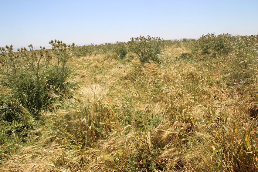
3708                                      N. Ouaadi et al.: C-band radar and in situ observations on wheat (central Morocco)

1   Introduction                                                    2011; El Hajj et al., 2016; Li and Wang, 2018; Ouaadi et
                                                                    al., 2020b) or based on linear or non-linear empirical regres-
The south Mediterranean region has been identified as a hot         sion (Gorrab et al., 2015; Ouaadi et al., 2020b) have been
spot of climate change (Giorgi, 2006; Giorgi and Lionello,          developed. The SSM derived from radar observations is also
2008; IPCC, 2014) that may worsen the water shortage al-            used to estimate RZSM (root zone soil moisture), a key vari-
ready affecting the region. Up to 90 % of available water           able in agronomy, through the combination with a land sur-
is dedicated to irrigation (Ministre de l’agriculture et peche      face model (Cho et al., 2015; Das et al., 2008; Dumedah
maritime du develpement rurale et des eaux et forets, 2018).        et al., 2015; Ford et al., 2014; Rodell et al., 2004; Sabater
Indeed, the predicted temperature rise that could reach 3 ◦ C       et al., 2006; Sure and Dikshit, 2019). The presence of a
by 2050 combined with precipitation decrease and increased          canopy above the soil results in two more contributions to
evapotranspiration could drastically increase the irrigation        the backscattered signal: the volume scattering and the atten-
requirements. The demand for water is also already increas-         uated signal by the canopy. The water content of vegetation
ing in response to an ever-growing population and to changes        influences the dielectric properties that in turn influence the
in agricultural practices – intensification, conversion to cash     radar backscatter from the vegetation (Ulaby et al., 1982).
crops and rise in irrigated areas (Ducrot et al., 2004; Fader       Based on these findings, some studies are focused on the re-
et al., 2016; Jarlan et al., 2016). The monitoring of irrigated     trieval of vegetation variables from SAR (synthetic aperture
crops and the optimization of water use are therefore of prime      radar) data such as aboveground biomass (Hosseini and Mc-
importance for the sustainability of the water resources in the     Nairn, 2017; Periasamy, 2018; Taconet et al., 1994) or even
Mediterranean region. This requires the implementation of           grain yield (Fieuzal et al., 2013; Patel et al., 2006). In ad-
methods to monitor the crop water status and the underlying         dition to the backscattering coefficient, the polarization ra-
soil moisture (Wang et al., 2012).                                  tio and the interferometric coherence have demonstrated po-
    Within this context, the observations from active space-        tentialities for the characterization of the vegetation includ-
borne sensors in the microwave domain (radar) have shown            ing height (Blaes and Defourny, 2003; Engdahl et al., 2001),
great potential for the monitoring of crops (Mattia et al.,         the vegetation cover fraction (Wegmuller and Werner, 1997),
2003; Ouaadi et al., 2020b; Picard et al., 2003). The potential     fresh aboveground biomass (Mattia et al., 2003; Veloso et al.,
of radar data for monitoring irrigated crops originates from        2017), aboveground biomass (Ouaadi et al., 2020b) and veg-
their high sensitivity to the water status of the surface includ-   etation water content (Ouaadi et al., 2020b). Other studies ac-
ing the water content of the aboveground biomass and the            knowledge the sensitivity of coherence to soil moisture (De
moisture of the upper soil layer (Ulaby and Dobson, 1986).          Zan et al., 2014; Scott et al., 2017). Recent research suggests
It is also sensitive to the structural properties of the observed   that radar observations could also provide valuable informa-
target including the size and orientation of the canopy ele-        tion on the canopy water status (Van Emmerik et al., 2015;
ments (leaves, steams, trunks) and the soil roughness. A key        Ouaadi et al., 2020d) for crop stress detection.
advantage of radar observations for monitoring crops, espe-            In situ measurements of vegetation and soil characteris-
cially those crops growing during the rainy season such as          tics are always needed to improve our understanding of the
wheat, is also that they are not prone to atmospheric per-          radar response, to develop and calibrate radiative transfer
turbations. Sentinel-1 provides for the first time since 2014       models, and to propose generic retrieval methods for the in-
backscattering coefficients at a resolution of 10 m and a re-       version of soil or vegetation variables. Nevertheless, in situ
visit time of 6 d compatible with the high dynamic of annual        data dedicated to these objectives are really specific in the
crops at the field scale, paving the way for an operational use     sense that, for instance, soil roughness is only of interest for
of C-band radar data for crop monitoring.                           understanding the physical principle of observations in the
    Nevertheless, radar signal is a complex mix of backscatter-     microwave domain. Likewise, aboveground biomass is often
ing from the soil and from the canopy that is often difficult to    measured by agronomists for crop modeling for instance, but
disentangle. The impact of any changes in the canopy struc-         the partition between dry and wet matter, a key variable for
ture such as the appearance of the heads during the head-           radar acquisition, is hardly ever performed. Indeed, the lat-
ing stage of wheat (Brown et al., 2003; El Hajj et al., 2019;       ter relies on heavy destructive measurements consisting in
Ulaby et al., 1986) or of the soil roughness may also dras-         cutting all the vegetation elements within square samples in
tically impact the backscattering response. These processes         the field and a double weighing before and after drying the
are not fully understood and not always properly reproduced         samples in an oven. In this paper, a recent, multiyear, com-
by the backscattering models.                                       plete database composed of processed Sentinel-1 SAR data
    The sensitivity of the backscattering coefficient to the sur-   (the backscattering coefficient and the interferometric coher-
face soil moisture (SSM) is widely documented in the liter-         ence); the Sentinel-2 NDVI; and measured variables on the
ature for bare or covered soils (Ezzahar et al., 2020; Ouaadi       soil, on the vegetation and on agricultural practices is made
et al., 2020c, b; Ulaby and Dobson, 1986; Zribi et al., 2014).      available. The in situ data include automatic measurements
Several retrieval approaches based on the inversion of a ra-        as well as observations carried out during measurement cam-
diative transfer model (Bai et al., 2017; Gherboudj et al.,         paigns once or twice every 15 d throughout the growing sea-

Earth Syst. Sci. Data, 13, 3707–3731, 2021                                          https://doi.org/10.5194/essd-13-3707-2021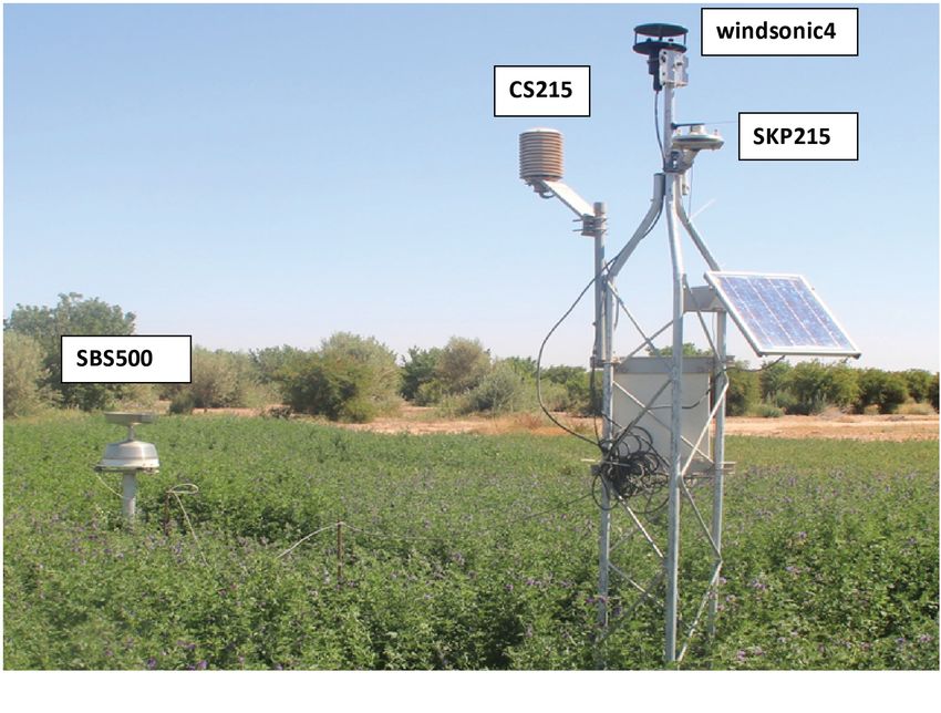
N. Ouaadi et al.: C-band radar and in situ observations on wheat (central Morocco)                                            3709

son. This database covers three wheat seasons (2016/17 to            2017/18 season, wheat in F2 was affected by specific grow-
2018/19) of three different irrigated fields (Ouaadi et al.,         ing conditions: (i) the development of adventices belonging
2020b). It is a unique and valuable data set that can be used        to the wild thistle family characterized by a horizontal struc-
for vegetation and soil moisture monitoring applications in-         ture, (ii) the seeding density being higher than in F1, and
cluding from radar observations. In addition, the multiyear          (iii) the seeding being a mixture of barley and wheat within
database can be useful for multiyear time series analysis. In        F2. This resulted in very long stems: 146 cm in F2 compared
the next section, an overview of the field location and a de-        to 110 cm in F1 in April 2018. Finally, these long stems in F2
tailed description of the variables, including field measure-        were laid down by the wind from 12 April 2018. A picture
ments and remote sensing data processing, are presented. In          of F2 during 2017/18 is provided in Appendix A (Fig. A1).
Sect. 3, the variables are experimentally and physically ana-        Although such exceptional growing conditions are not very
lyzed to assess the consistency of the data set. Conclusions         likely, it has been chosen to include this crop season in the
are provided in Sect. 4.                                             data set to cover different conditions of growth.

2     Study area and experimental sites                              3     Database

2.1    Study area                                                    3.1     Field data sets
The database described in this paper is collected in the Haouz       The field data sets consist of automatic measurements of soil
plain in the Tensift watershed, central Morocco (Fig. 1). This       moisture and weather data in addition to field surveys for sur-
plain is one of the most important plains in Morocco located         face roughness, biomass, vegetation water content, canopy
at 550 m above sea level and covers about 6000 km2 of which          height, the green leaf area index and the cover fraction. Ta-
2000 km2 is irrigated. The climate in the region is Mediter-         ble A1 in the Appendix summarizes the details of the 26,
ranean semi-arid, with annual average precipitation of about         18 and 16 field campaigns carried out during the 2016/17,
250 mm. The distribution of precipitation highlights a wet           2017/18 and 2018/19 seasons, respectively.
season with around 85 % of annual precipitation between Oc-
tober and April and a dry season from May to September.
                                                                     3.1.1    Soil moisture
The maximum average of temperature occurs during sum-
mer in July–August (about 35 ◦ C), and the minimum occurs            SSM is automatically measured every 30 min using time
in January (about 5 ◦ C) (Abourida et al., 2008). The average        domain reflectometry (TDR) sensors (Campbell Scientific
air humidity is about 50 %, and the reference evapotranspira-        CS616) using two sensors buried at a depth of 5 cm: one
tion ET0 is around 1600 mm yr−1 (Jarlan et al., 2015), which         under the drippers and another one between them. The av-
greatly exceeds the annual rainfall. The agricultural produc-        erage is computed in order to obtain a representative SSM
tion in the plain is not very diverse, focusing on cereals (51 %     value of the field. In addition, similar sensors are buried for
of the irrigated areas), olive trees (30 % of the irrigated area),   RZSM measuring at 25 and 35 cm of depth in F1 and F3,
and fodder production (9 %) and market gardening (2 %) for           while one sensor is buried at 30 cm in F2 because of the lack
cattle breeding, while the non-irrigated part of the plain is        of an additional sensor. Figure 2a illustrates an example of
cropped with rainfed wheat (Abourida et al., 2008). Wheat is         TDR sensors at different depths.
usually sown between November and January depending on                   TDR sensors are calibrated using the gravimetric tech-
precipitation distribution, even for irrigated fields, and on the    nique. The calibration is performed during the 2016/17 sea-
cultivar. Harvest usually occurs in May or June.                     son using samples taken from the first 5 cm from both fields
                                                                     F1 and F2, and then the calibrated equation is applied to F1,
2.2    Experimental sites                                            F2 and F3 data as the soil characteristics are similar and the
                                                                     same sensors are used. For that purpose, an aluminum core of
The database concerns three irrigated fields (F1, F2 and F3)         392.5 cm3 is used to collect samples at the TDR installation
located within a private farm in the province of Chichaoua           depths. Three samples are collected per day and per field dur-
located 65 km west of Marrakech city (Fig. 1). F1 and                ing 5 d chosen with different soil moisture conditions in or-
F2 are monitored during two successive growing seasons               der to cover a wide range of values (0.08 to 0.33 m3 m−3 ). A
(2016/17 and 2017/18), while F3 is monitored during the sea-         linear regression is established between the volumetric water
son 2018/19. The fields are sown using an automatic seed             content and the square root of the TDR time response (named
drill. They are irrigated using the drip technique. For all the      τ , in seconds) as follows:
fields, the wheat is cropped once a year during winter–spring
                                                                                       √
(see Table 1 for sowing and harvest dates). After harvest,           SSM = aTDR ×          τ + bTDR .                           (1)
the fields are generally used for cattle grazing until mid-July
when the plowing work starts. Table 1 summarizes some gen-           The calibrated values using data of both fields are aTDR =
eral information about the fields. Please note that during the       0.275 m3 m−3 s−0.5 and bTDR = −1.154 m3 m−3 . Figure 3

https://doi.org/10.5194/essd-13-3707-2021                                             Earth Syst. Sci. Data, 13, 3707–3731, 2021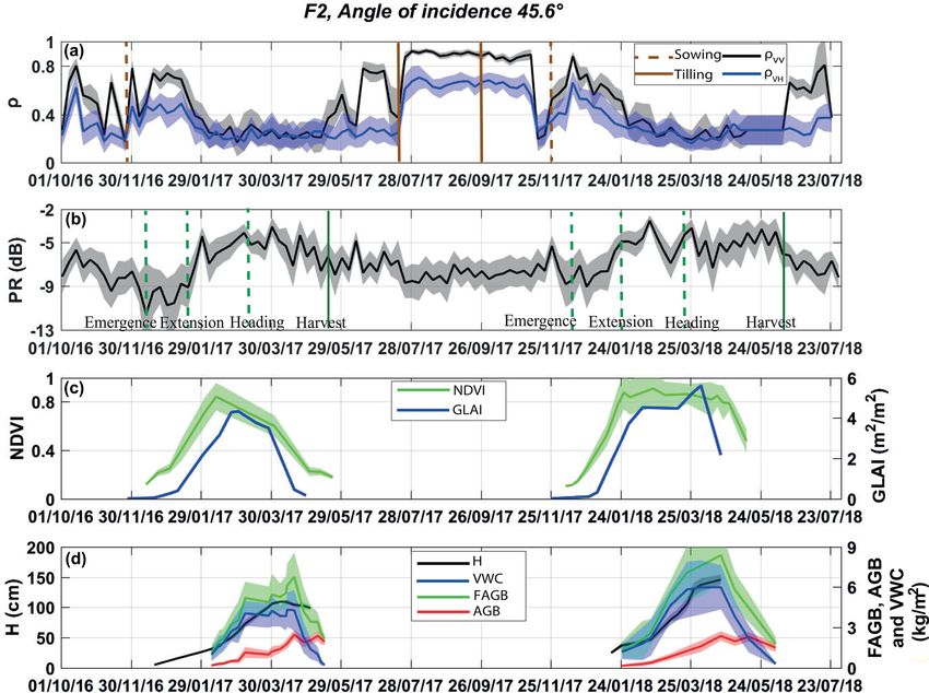
3710                                       N. Ouaadi et al.: C-band radar and in situ observations on wheat (central Morocco)

Figure 1. Location of the study fields: F1, F2 and F3 are drip-irrigated wheat plots in a private farm (Domaine Rafi) near the city of
Chichaoua in the Haouz plain, central Morocco.

Table 1. General information about the three fields.

                     Field   Area     Season           Sowing date           Harvest date     Irrigation   Sand   Clay
                             (ha)                                                                           (%)    (%)
                     F1        1.5    2016/17 &        25 November 2016,     16 May 2017,     Drip         32.5   37.5
                     F2        1.5    2017/18          27 November 2017      8 June 2018      technique
                     F3         12    2018/19          4 November 2018       6 June 2019

illustrates the calibration results with all the samples dis-              eter (L) corresponds to the distance between measurements
played. The statistical metrics are the correlation coefficient            from which the heights between points are statistically inde-
R = 0.97, root mean square error RMSE = 0.018 m3 m−3                       pendent. This parameter provides a horizontal description of
and no bias. When considering both fields separately, the                  the ground surface roughness, more specifically the organi-
results for (F1, F2) are R = (0.90, 0.94), RMSE = (0.023,                  zational structure and spatial continuity of the microtopogra-
0.01) m3 m−3 and bias = (−0.002, 0.003) m3 m−3 .                           phy (Nolin et al., 2005). Over the three studied fields, mea-
   The calibrated equation is also applied for the RZSMs                   surements of the surface roughness are taken during the first
assuming that the soil properties are the same at different                stage of wheat (from emergence to early tillering) when the
depths. Figure A2 in Appendix A illustrates an example of                  ground is not totally covered by the canopy. We used a pin
an RZSM time series in F1.                                                 profiler of 1 m length, composed of a set of 53 metal needles
                                                                           of equal length every 2 cm (Fig. 2b). A total of 16 sample
3.1.2   Surface roughness                                                  pictures are taken per field and per date including 8 pictures
                                                                           parallel and 8 pictures perpendicular to the rows’ direction.
Surface roughness characterizes the micro-variation in the                 The pictures are taken using a Canon 6EOS 600D equipped
ground surface elevation within a given area/field (Allmaras               with a Tamron lens (Model A14).
et al., 1966). It affects particularly the SAR signal and to a                The images are processed in MATLAB based on the de-
lesser extent the visible and near infrared (Girard and Gi-                tection of the top position of each needle. hrms and L are
rard, 1989). The two parameters that characterize the sur-                 computed from the auto-correlation function, and then the
face roughness are the root mean square height (hrms ) and                 average per direction, per field and per date is computed. For
the correlation length (L). hrms provides a vertical descriptor            illustration, Fig. 4 shows the time series of hrms and L pa-
of ground roughness by measuring the elevation of the sur-                 rameters computed separately for each direction for F1 and
face along one or more observation lines and calculating the
standard deviation of the recorded values. The second param-

Earth Syst. Sci. Data, 13, 3707–3731, 2021                                                  https://doi.org/10.5194/essd-13-3707-2021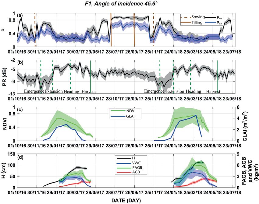
N. Ouaadi et al.: C-band radar and in situ observations on wheat (central Morocco) 3711
Figure 2. Examples of (a) TDR sensors installed at different depths and (b) a pin profiler picture taken over one of the plowed field with
drip irrigation tubes installed.
Table 2. Average values of the roughness parameters (eight samples are gathered per field and per direction).
F1 F2 F3
hrms L hrms L hrms L
(cm) (cm) (cm) (cm) (cm) (cm)
2016/17 Parallel 0.92 5.02 1.19 5.77
Perpendicular 1.34 5.88 1.19 5.8
Average 1.13 5.45 1.19 5.78
2017/18 Parallel 0.89 5.44 1.1 5.88
Perpendicular 1.16 7.4 1.12 6.6
Average 1.02 6.42 1.11 6.24
2018/19 Parallel 0.83 6.54
Perpendicular 0.96 7.32
Average 0.89 6.93
F2 during the season 2017/18, while the average values per 3.1.3 Biomass and water content
season are summarized in Table 2 for F1, F2 and F3.
Biomass and water content are two biophysical parameters
Based on the range of hrms measurements
of crucial importance in different agricultural applications in-
(0.83 < hrms < 1.35), it can be clearly seen that the fields are
cluding particularly plant stress monitoring, radar backscat-
characterized by a slightly rough or smooth surface, which
tering response, crop yield and evapotranspiration model-
is generally the case for disc-tilled fields. After sowing,
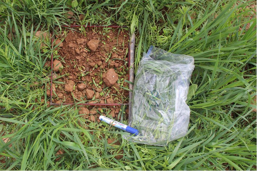
ing. Within each field, eight samples are collected once a
a slight change is observed at the start of the crop season
week/every 2 weeks during the growing season. The sam-
(28 December 2017; see Fig. 4). At that time, the soil has
ples are chosen randomly so that the average is representa-
just been prepared for sowing and rows are directly exposed
tive of the plot. A quadrate of an area of 0.0625 m2 is used
to rain. The fact that the rows are still visible in the field also
for the sampling (Fig. 5). The samples are weighed first in the
explains the differences observed between both directions
field to obtain fresh aboveground biomass (FAGB). The cor-
early in the season. This anisotropy disappeared quickly
responding aboveground biomass (AGB) expressed in kilo-
with irrigation, rainfall and plant growth. hrms and L are
grams of dry matter per square meter is determined at the
almost constant from early January onwards. Indeed, it has
laboratory by drying the samples in an electric oven at 105 ◦ C
been shown that after sowing, roughness is affected by very
for 48 h. The vegetation water content (VWC) is thus com-
limited temporal variations (Bousbih et al., 2017) as no soil
puted as the difference between FAGB and AGB (Gherboudj
works occur after sowing. It is usually kept constant during
et al., 2011).
the crop season (El Hajj et al., 2016; Gherboudj et al., 2011;
Gorrab et al., 2015; Ouaadi et al., 2020b).
https://doi.org/10.5194/essd-13-3707-2021 Earth Syst. Sci. Data, 13, 3707–3731, 2021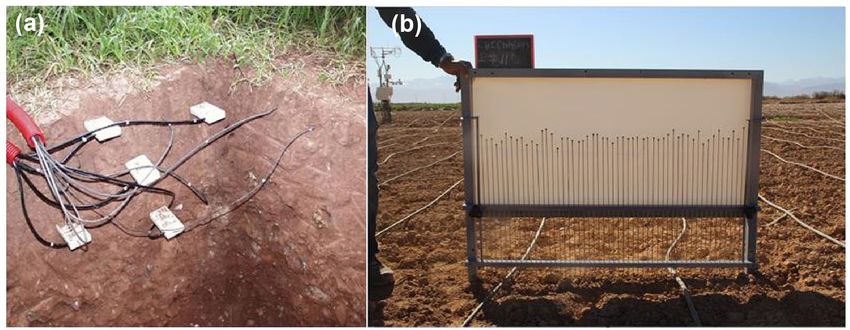
3712                                       N. Ouaadi et al.: C-band radar and in situ observations on wheat (central Morocco)

                                                                       Figure 5. Photo taken during a measurement campaign illustrating
                                                                       a sample of aboveground biomass measurement.

                                                                       (Fig. 6b) using MATLAB software following the method de-
Figure 3. Surface soil moisture measured by TDR versus gravimet-       scribed in Duchemin et al. (2006) and Khabba et al. (2009).
ric measurements using samples collected in both fields F1 and F2      The eight photos per date and per field are taken using a
during the 2016/17 growing season. The solid blue line is the linear   Canon 6EOS 600D camera with a SIGMA 4.5 mm F2.8 EX
regression, and the dashed line is Y = X.                              DC circular fisheye HSM (Fig. 6a). Photos are taken in op-
                                                                       timal lighting conditions to avoid shadow effects and over-
                                                                       exposure phenomena which make classification more diffi-
                                                                       cult. The algorithm is based on the binarization of the hemi-
                                                                       spherical images by thresholding a greenness index. Next,
                                                                       the useful part of the images is extracted by masking the op-
                                                                       erator and the high viewing angles (> 75◦ ) (Fig. 6c). Finally,
                                                                       the ground-covered area is extracted on concentric rings as-
                                                                       sociated with fixed viewing angles, and the average of all
                                                                       pictures is the field GLAI. Using the same process, FC is cal-
                                                                       culated as the ratio of the vegetation pixel number to the total
                                                                       pixel number.

                                                                       3.1.5   Irrigation and weather data
                                                                       F1, F2 and F3 are irrigated using the drip technique. Irri-
                                                                       gation quantities are determined by the farmer by estimat-
                                                                       ing the daily evapotranspiration under standard conditions
                                                                       (ETc ) in the region computed using the FAO 56 model sim-
                                                                       ple approach (Allen et al., 1998). The cumulative ETc for
Figure 4. Time series of hrms and L computed from parallel and
perpendicular measurements separately for F1 and F2 during the         a given period (usually 1 week) is applied during one or
season 2017/18.                                                        more events per week depending on the farmer’s constraints
                                                                       (e.g., availability of workforce) and on the weather con-
                                                                       ditions (e.g., occurrence of rain). The irrigation pipes are
3.1.4   Canopy height, green leaf area index and cover                 spaced by 0.7 m, while the distance between the drippers
        fraction                                                       along the pipe is 0.4 m. In F1 and F2, the flow rate of each
                                                                       dripper is 7.14 mm h−1 . The irrigation takes place for about
The canopy height (H ), green leaf area index (GLAI) and               105 min (12.53 mm). A flowmeter mounted downstream of
cover fraction (FC ) are measured every week during the                a valve allowed an accurate collection of irrigation volumes.
growing season. Values from 11 different places are aver-              F2 and F3 are irrigated according to FAO recommendations,
aged and considered a representative measure of the field. H           while F1 is stressed voluntarily. The stress involved in F1
is simply measured using a measuring tape, while the GLAI              is during the first season (2016/17) only. By contrast, the
and FC are computed by processing hemispherical photos                 2017/18 season was wet, so there is no clear stress observed

Earth Syst. Sci. Data, 13, 3707–3731, 2021                                             https://doi.org/10.5194/essd-13-3707-2021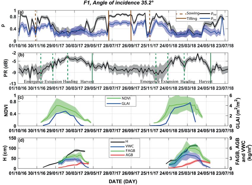
N. Ouaadi et al.: C-band radar and in situ observations on wheat (central Morocco)                                                    3713

Figure 6. (a) The 4.5 mm F2.8 EX DC circular fisheye HSM, (b) a hemispherical photo, and (c) the result of the processing after binarization
and after masking the operator and the high viewing angles (> 75◦ ).

                                                                         3.2     Remote sensing data sets

                                                                         3.2.1    Sentinel-1

                                                                         Sentinel-1A (S1A) and Sentinel-1B (S1B) are Earth obser-
                                                                         vation satellites developed for the Copernicus initiative and
                                                                         launched by the European Space Agency in April 2014 and
                                                                         April 2016, respectively. During full operation, S1A and S1B
                                                                         are maintained in the near-polar Sun-synchronous orbit at
                                                                         693 km in altitude, phased 180◦ , providing a revisit time
                                                                         of 6 d (Torres et al., 2012). Sentinel-1 (S1) is a synthetic
                                                                         aperture radar operating at the C-band with a frequency of
                                                                         5.33 GHz, mapping the entire world in 175 orbits per cycle.
                                                                         The main operational imaging mode is the Interferometric
                                                                         Wide (IW) swath mode. IW acquires data with a wide swath
                                                                         of 250 km with high geometric (azimuth resolution 20 m and
                                                                         ground range resolution 5 m) and radiometric resolution (Eu-
Figure 7. Automatic weather station installed in an alfalfa field near   ropean Space Agency, 2012). The IW mode supports opera-
F1, F2 and F3.                                                           tion in single and dual polarization (HH, VV, HH–HV and
                                                                         VV–VH) and covers a range of incidence angles between 31
                                                                         and 46◦ . The product is composed of three sub-swaths ac-
on the field. The irrigation dates and amounts in F1 and                 quired with the TOPSAR imaging technique which signifi-
F2 during both seasons are made available throughout this                cantly reduces the scalloping effect (De Zan and Guarnieri,
database, while the irrigation in F3 is not available.                   2006).
   The weather data including precipitation, air temperature,               Level-1 products are systematically processed and avail-
relative humidity, solar radiation, and wind speed and direc-            able within 24 h, free of charge from the Copernicus Open
tion are collected by an automatic weather station installed             Access Hub website (https://scihub.copernicus.eu, last ac-
over an alfalfa field near the studied fields (Fig. 7). The              cess: 19 July 2021). The website provides data for two types
weather station provides continuously meteorological data                of products: GRDH (Ground Range Detected High Resolu-
every 30 min. The Campbell sensor CS215 is used to mea-                  tion) and SLC (Single Look Complex).
sure the air temperature and the relative humidity (Fig. 7).                In this database, 561 GRDH and SLC products are pro-
The global solar radiation and the wind direction and speed              cessed (Table 3). Among them, 124 images are acquired over
are measured using the Campbell SKP215 and Campbell                      F3 during the 2018/19 growing season and 437 over F1 and
WindSonic4, respectively. The precipitation is measured us-              F2 from 1 October 2016 to 31 July 2018, along the ascend-
ing the rain gauge (Campbell SBS500) shown in Fig. 7.                    ing no. 118 (221 images) and descending no. 52 (216 images)
                                                                         relative orbits. This period includes two agricultural seasons
                                                                         in addition to the summer period.

https://doi.org/10.5194/essd-13-3707-2021                                                Earth Syst. Sci. Data, 13, 3707–3731, 2021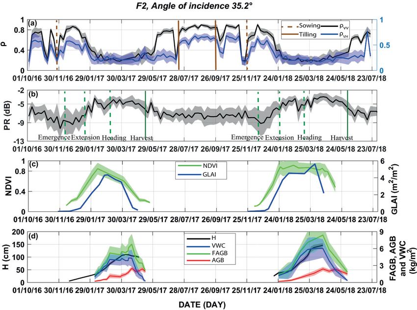
3714                                        N. Ouaadi et al.: C-band radar and in situ observations on wheat (central Morocco)

Table 3. Characteristics of the sentinel-1 products processed over the three fields for the monitored periods.

            Field        Season               Relative orbit    Incidence      Relative              Overpass        Product   Number of
                                                    number      angle          orbit                 time (UTC)                  images
            F1 and F2    October 2016–                  118     45.6◦          Ascending             18:30           GRDH           112
                         July 2018                                                                                   SLC            109
                                                          52    35.2◦          Descending            06:30           GRDH           110
                                                                                                                     SLC            106
            F3           November 2018–                 118     45.6◦          Ascending             18:30           GRDH            32
                         May 2019                                                                                    SLC             31
                                                          52    35.2◦          Descending            06:30           GRDH            31
                                                                                                                     SLC             30

Backscattering coefficient                                                  F3, respectively, with a mean standard deviation of around
                                                                            1.55 dB. In order to visualize data dynamics, backscattering
GRDH products are provided by ESA with a square                             coefficients are converted into decibels.
pixel size and contain only the intensity information. The
backscattering coefficients are extracted using the Orfeo
                                                                            Interferometric coherence
ToolBox (CNES, 2018). The processing procedure consists
of three steps (Frison and Lardeux, 2018):                                  Sentinel-1 SLC products are provided in slant-range geom-
                                                                            etry. They contain three sub-swath images: IW1, IW2 and
  1. Thermal noise removal. The SAR product contains not                    IW3. Each sub-swath is composed of nine bursts with black-
     only the useful signal but also the unwanted noise dis-                fill demarcation. By contrast with GRDH, both intensity in-
     turbing the information contained in the intensity im-                 formation and phase information are kept. The phase infor-
     ages, especially when the backscattered power is low.                  mation is used for the computation of interferometric coher-
     The thermal noise is an additive noise. The compensa-                  ence. SAR interferometry consists of correlating two images
     tion for this noise can be performed by subtracting the                acquired from two positions in space slightly separated from
     scaled noise power using the calibrated noise vectors                  each other (with two radars mounted on the same platform)
     provided by ESA.                                                       or at different times by exploiting repeated orbits of the same
  2. Calibration. The calibration step aims to convert the                  satellite such as for Sentinel-1. Thanks to its high tempo-
     digital accounts into a physically interpreted parame-                 ral resolution (6 d per orbit), the interferometric coherence
     ter: the backscattering coefficient. A calibration vector              is computed from two consecutive acquisitions of the same
     included in the GRDH products contains the necessary                   orbit.
     information to convert the digital values to the backscat-                 The interferometric coherence, given by Eq. (2), for a local
     tering coefficient.                                                    neighborhood of N pixels, is generated by cross-multiplying,
                                                                            pixel by pixel, the first SAR image zi with the complex con-
  3. Terrain correction. S1 SAR data are sensed with a view-                jugate zi0 ∗ of the second (Bamler and Hartl, 1998; Touzi et al.,
     ing angle greater than zero which induces distortion in                1999).
     the products because of the lateral viewing geometry.                             N
                                                                                             zi · zi0 ∗
                                                                                       P
     The “Terrain correction” module is used to compensate
                                                                                      i=1
     for these distortions and obtain as many images as pos-                ρ=s                                                            (2)
     sible with real geometric representation. The images are                      N                 N
                                                                                                                 2
                                                                                          |zi |2 ·         zi0
                                                                                   P                 P
     projected on the Earth’s surface using a digital elevation                    i=1               i=1
     model (DEM). The SRTM (Shuttle Radar Topography
     Mission) DEM of 30 m resolution is used according to                   The interferometric coherence |ρ| varies between zero (inco-
     the method described in Small and Schubert (2008).                     herence) and 1 (perfect coherence). The interferometric co-
                                                                            herence is related to the movements of the scatterers within
SAR images are affected by the speckle noise, which is                      a given canopy. It decreases (loss of coherence) in the case
mainly due to the relative phase of individual scatters within              of dense vegetation, while high values are obtained over bare
a resolution cell. Many filters have been developed to remove               soils. Loss of coherence could be caused by the temporal in-
the speckle noise although the best filter is the spatial aver-             terval between acquisitions, orbit errors, vegetation develop-
age. The presented database is generated using a simple av-                 ment/movement or processing errors. The random disloca-
erage per field of 120, 121 and 1100 pixels for F1, F2 and                  tion of scatters because of the weather (wind and rain) or the

Earth Syst. Sci. Data, 13, 3707–3731, 2021                                                       https://doi.org/10.5194/essd-13-3707-2021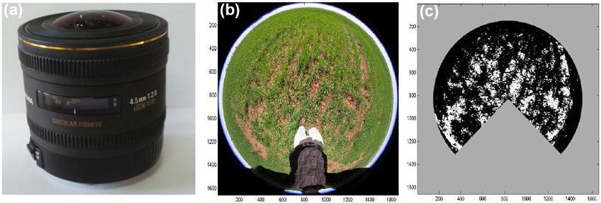
N. Ouaadi et al.: C-band radar and in situ observations on wheat (central Morocco)                                           3715

plants’ growth is the main cause of the temporal decorrela-               Model for Atmospheric Correction (SMAC) method by
tion.                                                                     Rahman et al. (1994). The concentrations of the ozone,
   The Sentinel application platform SNAP is used to com-                 the oxygen and the water vapor are obtained from satel-
pute the interferometric coherence from S1 SLC products in                lite data (ozone) and meteorological data (water vapor,
five steps (Veci, 2015):                                                  pressure).

 1. Apply-Orbit-File. This module is applied for a better es-          2. The detection of the clouds (and clouds’ shadows) is
    timation of the position and speed of the satellite us-               based on the multi-temporal cloud detection method
    ing the orbit state vector. Preliminarily, a predicted orbit          proposed by Hagolle et al. (2010).
    state vector is contained in the metadata, but it is not ac-
    curate. The precise orbit is made available 1 month after          3. The estimation of the aerosol optical thickness (AOT)
    data acquisition at the latest. For this reason, the auto-            relies on a hybrid method merging the criteria of a
    matic download in SNAP is used in order to update the                 multi-spectral method with the multi-temporal tech-
    orbit state vectors.                                                  nique developed initially for the VENµS satellite mis-
                                                                          sion by Hagolle et al. (2010). The AOT is used along
 2. Back-Geocoding. The two images need to be co-                         with the surface altitude, the viewing geometry and the
    registered. One of the images is the master, and the                  wavelength in the parameterization of look-up tables for
    other is the slave. This step ensures that each pixel of              the conversion of TOA reflectances already corrected
    the slave image is aligned with the corresponding pixel               in step 1 into surface reflectances. The look-up tables
    in the master image so that both pixels contain contribu-             are provided by the successive orders of scattering code
    tions from the same target. The DEM is required for the               (Lenobel et al., 2007) used in the modeling of molecular
    Back-Geocoding step; SNAP allows us either to enter it                and aerosol scattering effects. A different look-up table
    manually or to download it automatically.                             is computed for each aerosol model.

 3. Coherence. This module in SNAP allows the computa-             Data are downloaded from the Theia site. Among the avail-
    tion of the interferometric coherence between the two          able products, only the products non-covered with clouds
    images for a given local neighborhood. In order to ob-         are used corresponding to 10, 25 and 26 images for the
    tain a square pixel of 13.95 m, azimuth × range is fixed       2016/17, 2017/18 and 2018/19 agricultural seasons, respec-
    to 3 × 15 in the processing.                                   tively. Please note that during the season 2016/17, only S2A
                                                                   was in the orbit which explains the limited number of im-
 4. TOPSAR-Deburst. The black fills in between bursts are          ages (10). Next, the normalized difference vegetation index
    deleted separately for both polarization images (VV and        (NDVI) corresponding to each pixel is computed from band
    VH).                                                           4 and 8. An average per field is used to compute the time
                                                                   series of each field.
 5. Terrain-Correction. Finally, the processed images are
    projected on the Earth’s surface using a DEM.
                                                                   4     Data analysis
3.2.2   Sentinel-2 NDVI
                                                                   4.1    Vegetation variables
Sentinel-2 optical satellites S2A and S2B were launched
                                                                   In this section, the relationships between the different vari-
by ESA in June 2015 and March 2017, respectively. They
                                                                   ables (GLAI, FAGB, AGB, VWC and H ) that character-
are placed in opposition on the same orbit at an altitude of
                                                                   ize the vegetation growth and development are first inves-
800 km. Sentinel-2 provides data every 5 d with a width of
                                                                   tigated. These relationships are extensively used for different
290 km and a resolution of 10 to 60 m according to spec-
                                                                   applications such as the calibration of backscattering models
tral bands (13 bands) ranging from visible to the medium in-
                                                                   and the development of retrieval approaches (Chauhan et al.,
frared. The National Centre for Space Studies (CNES) pro-
                                                                   2018). Several land surface or crop models rely on empiri-
vides Level-2A products atmospherically corrected free of
                                                                   cal relationships to predict FC or H as well (Bigeard et al.,
charge via PEPS (https://peps.cnes.fr/, last access: 19 July
                                                                   2017; Castelli et al., 2018). Other agricultural models com-
2021) or the Theia website (https://theia.cnes.fr/, last access:
                                                                   pute AGB from the GLAI using linear or polynomial rela-
19 July 2021). Data are corrected for atmospheric effects by
                                                                   tionships (Major et al., 1986; Petcu et al., 2003). Figure 8
the Center for the Study of the Biosphere from Space (CES-
                                                                   displays the resulting relationships using data from F1 by
BIO) using the MAJA chain (Hagolle et al., 2015). The at-
                                                                   selecting only the 2016/17 season for illustrative purposes.
mospheric corrections are performed in three steps:
                                                                   These relationships are computed separately based on the
 1. The satellite top-of-atmosphere (TOA) reflectances are         data recorded before and after the peaks of the GLAI and
    corrected for the absorption by the atmospheric gas            FAGB.
    molecules using the absorption part of the Simplified

https://doi.org/10.5194/essd-13-3707-2021                                           Earth Syst. Sci. Data, 13, 3707–3731, 2021
3716                                     N. Ouaadi et al.: C-band radar and in situ observations on wheat (central Morocco)

Figure 8. Scatterplots of the relationships between wheat measured variables: FAGB, AGB, VWC, H , GLAI and FC . Data are presented
separately using the maximum of the GLAI and FAGB as thresholds: data < max GLAI are in black; data < max FAGB (and > max GLAI)
are in grey, and data > max FAGB (and > max GLAI) are in blue.

    The nature of the relationship changes depending on the        the GLAI and FAGB is observed. This is probably related to
structure (biomass variables) or on the greenness of the plant     the senescence of the lower leaves, which leads to an earlier
(GLAI). The biomass variables (FAGB, AGB and VWC)                  drop of the GLAI than of FAGB. Between the peaks of the
and H increase up to the biomass peak. Afterwards, a re-           GLAI and FAGB, the GLAI decreases while (i) AGB and
verse evolution can be observed, characterized in particular       H increase and (ii) FAGB increases slightly while VWC is
by a decorrelation between FAGB/VWC and AGB. This is               almost constant. After the FAGB peak, AGB goes on increas-
mainly related to the senescence process of the vegetation;        ing due to grain filling while the VWC decreases due to dry-
the leaves begin to dry progressively with the start of the        ing of the plant. FAGB, which is the sum of AGB and VWC,
grain filling, so the sap flow (water, carbohydrates, proteins     is almost constant.
and mineral salts) migrates to the heads at the top of the plant
(Farineau and Morot-Gaudry, 2018). Indeed, VWC and AGB
                                                                   4.2     Radar data
are highly correlated until the vegetation peak (the correla-
tion coefficient is R = 0.94 before the peak and R = −0.20         The time series of the backscattering coefficient, the polar-
afterwards), while FAGB being dominated by the plant water         ization ratio and the interferometric coherence are analyzed
content is highly correlated with VWC during the whole crop        here for two agricultural seasons and a summer period on F1
season (R = 0.99 before the peak, and R = 0.98 afterwards).        and F2 and at two incidence angles (35.2 and 45.6◦ ).
Likewise, H is highly correlated to FAGB, VWC and AGB
until the vegetation peak (R > 0.97) when H remains at its
                                                                   4.2.1    The backscattering coefficient
maximum value while AGB continues to increase with grain
filling and VWC and FAGB decrease because of the veg-              Figure 9 displays the time series at 45.6◦ in F2 for illustra-
etation drying. The relationship of these variables (FAGB,         tive purposes: (a) backscattering coefficient at VV polariza-
AGB, VWC and H ) with the GLAI and FC is quite different.                 0 ); (b) backscattering coefficient at VH polarization
                                                                   tion (σVV
The curves are of a parabolic shape with a maximum reached            0
                                                                   (σVH ) as well as wheat phenological stages; (c) SSM, air
around the GLAI peak. A timing shift between the peaks of          temperature, irrigation and rainfall. Figures A3–A5 in Ap-

Earth Syst. Sci. Data, 13, 3707–3731, 2021                                         https://doi.org/10.5194/essd-13-3707-2021
N. Ouaadi et al.: C-band radar and in situ observations on wheat (central Morocco) 3717
pendix A show the same time series in F1 and F2 at 35.2◦ The low variation observed on F1 during the 2016/17 sea-
and F1 at 45.6◦ , respectively. The backscattering coefficients son is mainly related to the limited development of vegeta-
reveal a strong seasonal signal with two cycles. The first cy- tion because of the triggered water stress. Likewise, the dif-
cle takes place from sowing to the heading stage, and the ference between the two seasons in F2 is related to a higher
second takes place from heading to harvest with the mini- density of grown seeds and wetter conditions in the 2017/18
mum reached around the heading stage. The highest values season compared to 2016/17 (the amount of rainfall dur-
at 35.2◦ are observed in the first cycle, while at 45.6◦ , σ ◦ ing the growing season – from sowing to harvest – reached
is higher during the second peak. The maximum values of 167.23 mm in 2017/18 while only 69.94 mm is recorded in
0 reached the same value for F1 and F2, while higher
σVV 2016/17). With the drying of the head layer, the backscatter-
values are observed on F2 at VH. σVV 0 is more sensitive to ing decreases again at the end of the season to reach the lower
soil moisture variation until mid-January, corresponding to observed values. Indeed, as the head layer dries, the vegeta-
the tillering stage, when the soil is not yet fully covered by tion becomes transparent to the signal. The soil is also dry
vegetation. Although it is agreed that the signal during this at the end of the season because irrigation is stopped. These
period is governed by the dynamics of soil moisture, its be- low values remain until the first deep plowing on 11 July,
havior differs from one site to another, giving the difference when a sharp increase is observed because of a drastic change
in soil hydric conditions and surface roughness. After this in soil roughness. Hereafter, the signal is again stable until
period, the signal behavior is similar to the profiles obtained the seedling preparation work for the next 2017/18 season
by Cookmartin et al. (2000), El Hajj et al. (2019), Nasrallah (22 November).
et al. (2019) and Veloso et al. (2017). It decreases gradu-
ally from the early tillering until the heading stage (around 4.2.2 The interferometric coherence and the
13 March) by about 10 dB on F2 and 5 dB on F1 because polarization ratio
of the attenuation by the canopy during the development of
the stems (extension stage) (Cookmartin et al., 2000; Mattia Figure 10 displays the time series at 45.6◦ in F2 of the (a) in-
et al., 2003; Picard et al., 2003; Wang et al., 2018). Obvi- terferometric coherence at VV (ρVV ) and VH (ρVH ) polariza-
ously, the attenuation is more important at VV polarization tions together with sowing and tilling dates; (b) polarization
because of the vertical structure of wheat (stems) in line with ratio (PR = σVH0 /σ 0 ), as well as wheat phenological stages;
VV
the results of Fontanelli et al. (2013), Picard et al. (2003) and (c) Sentinel-2 NDVI and measured GLAI; and (d) measured
Wang et al. (2018). The response of σVH 0 to SSM variation FAGB, AGB, VWC and H . Likewise, Figs. A6–A8 in Ap-
and canopy attenuation is lower than for σVV 0 . After the head- pendix A display the time series in F1 and F2 at 35.2◦ and
ing stage, the signal starts to increase again. This is clearer on F1 at 45.6◦ , respectively. The time series of ρVV and ρVH
F2 than on F1 and at 45.6◦ than at 35.2◦ . The heading stage is follows a similar evolution. Before sowing, coherence is at
the phenological stage of wheat when the spike or head starts its highest value corresponding to 0.9 for ρVV and 0.7 for
emerging out from the leaf sheath. This change in the struc- ρVH (Fig. 10a). These values express a dominance of co-
ture of the canopy shields the stems from the radar signal herent scattering, corresponding to the response of bare soils
through the appearance of a thick, wet, top layer composed composed of big rocks. Indeed, during the summer, the plots
of the heads. The C-band wavelength penetrates this layer are subjected to deep plowing which yields big clods that re-
only, resulting in increased volume scattering, while attenua- sist any change in surface structure caused by climatic factors
tion becomes low. This effect is stronger for F2 than for F1, at such as wind or rain. The second tilling breaks up the clods
VH than at VV and at 45.6◦ than at 35.2◦ . This increase was for the next seeding. Soil works and farming activities induce
first reported by Ulaby and Batlivala (1976). Subsequently, a large decrease in coherence in line with the observation of
Ulaby et al. (1986) suggested that an additional term must be Wegmuller and Werner (1997). The surface roughness is a
added to the traditional three-term model (vegetation volume main parameter that influences not only the amplitude at the
diffusion, soil attenuation and soil–vegetation interaction) to C-band but also the phase. Indeed, abrupt drops are observed
properly represent wheat backscattering after heading. Later around each sowing event and tilling works (vertical brown
on, similar behavior was observed and attributed by numer- lines in Fig. 10a).
ous authors to the appearance of the heads followed by the After sowing, the evolution is similar to that of the pro-
grain (Brown et al., 2003; El Hajj et al., 2019; Mattia et al., files obtained by Blaes and Defourny (2003) and Engdahl
2003; Patel et al., 2006; Veloso et al., 2017). The exceptional et al. (2001). The interferometric coherence increases from
growing conditions in F2 during the 2017/18 season is behind 0.15 to 0.7 and then starts to decrease slightly from the emer-
the origin of the observed plateau of the backscattering coef- gence of wheat, becoming almost constant after stem ex-
ficient which remains quite stable until harvest. This is due to tension with values < 0.3 corresponding to the noise level.
a significant contribution of volume scattering which is a be- Indeed, using the ERS-2–Envisat Tandem mission, Santoro
havior that characterizes a crop developing a random canopy et al. (2010) demonstrated that coherence measurements of
structure in relation to the numerous and dense adventices as vegetated fields are always below the level of bare soil co-
already highlighted (see picture Fig. A1 in Appendix A). herence. Actually, the interferometric coherence is known to
https://doi.org/10.5194/essd-13-3707-2021 Earth Syst. Sci. Data, 13, 3707–3731, 20213718 N. Ouaadi et al.: C-band radar and in situ observations on wheat (central Morocco) Figure 9. Time series of the backscattering coefficient at VV (a) and VH (b) polarizations on F2 at a 45.6◦ incidence angle during the period from 1 October 2016 to 31 July 2018. The tilling works and phenological stages of wheat are superimposed in panels (a) and (b), respectively. The air temperature, surface soil moisture (SSM), irrigation and rainfall are displayed in panel (c). Figure 10. Time series of the interferometric coherence at VV and VH polarizations (a) and the polarization ratio (b) on F2 at a 45.6◦ incidence angle during the period from 1 October 2016 to 31 July 2018. The tilling works and phenological stages of wheat are superimposed in panels (a) and (b), respectively. The NDVI and measured GLAI are displayed in panel (c). Measured H , FAGB, VWC and AGB are plotted in panel (d). Time series are presented by mean values (solid lines) and standard deviations (shading surrounding the solid lines). Earth Syst. Sci. Data, 13, 3707–3731, 2021 https://doi.org/10.5194/essd-13-3707-2021
N. Ouaadi et al.: C-band radar and in situ observations on wheat (central Morocco)                                          3719

decrease exponentially with wheat growth (Lee et al., 2012).       higher saturation values than the other relationships (∼ 55 %
Vegetation growth and random dislocation of scatters cause         of H range which is about 77 cm). By contrast, a visual in-
a degradation of coherence (Blaes and Defourny, 2003; En-          spection of Fig. 11d, i and n shows that relationships with
gdahl et al., 2001; Wegmuller and Werner, 1997), especially        the NDVI are poorer when using data of the whole growing
under wind and rain effects. Between sowing and emergence,         season. The dispersion is strong over the season. Data before
the observed variation is assumed to be related to the installa-   and after the maximum development can be distinguished,
tion of irrigation drippers that took place up to 2 weeks after    particularly using ρVV and to a lesser extent ρVH . Figure 11i
sowing. The changes that occur between the harvest and the         and n show that a linear relationship exists between the NDVI
first tilling could be attributed to livestock grazing, a com-     and SAR data using data before maximum development only,
mon practice in the region after wheat harvest, which could        i.e., when the vegetation is still green. During the beginning
change the surface roughness.                                      of the season, the slope of ρVV –NDVI and ρVH –NDVI is low
   The polarization ratio (PR) is closely related to the           compared to the other vegetation variables. This is because
biomass dynamic. Both increase from emergence to heading           the NDVI increases faster around the emergence of wheat
and then start to decrease until harvest. The maximum timing       while ρVV is still high because of the low vegetation cover
is around the middle of April. The significant differences in      fraction at this time. The hysteresis effect observed after the
biophysical parameters between F1 and F2 are due to irriga-        maximum of vegetation development is due to the senes-
tion, as already highlighted for the backscattering coefficient    cence of the leaves when the NDVI starts decreasing while
time series. Likewise, the difference between the two seasons      ρVV and ρVH are stable at low values.
in F2 is related to a higher sowing density and wetter condi-         When considering SAR data at a 45.6◦ incidence angle
tions in the 2017/18 season compared to 2016/17. As shown          (Fig. A9), a similar behavior to that shown in Fig. 11 is ob-
in Fig. 8, the time series of FAGB and VWC are in line with        served with AGB, VWC, H and the NDVI. The same hys-
AGB and H up to the peak of FAGB and then decrease to-             teresis and scattering are observed for the NDVI although
gether while AGB continues to increase and H remains at its        higher correlations are obtained. Similarly, ρVV is better cor-
maximum value. FAGB and VWC drop at the same time but              related to vegetation variables than ρVH and PR. By con-
50 d later when compared to the GLAI and NDVI and about            trast, the GLAI is better correlated with SAR variables than
15 d before the backscattering coefficient.                        H . The PR–GLAI relationship is more scattered than at
                                                                   35.2◦ while the ρVV –GLAI relationship has the best met-
4.3   Relationship between SAR data and vegetation
                                                                   rics (Rs = 0.82, and R 2 = 0.73) with a higher saturation value
      variables
                                                                   around 50 % of the GLAI range (3 m2 m−2 ).
                                                                      Unlike PR, the metrics at both 35.2 and 45.6◦ are stable
The polarization ratio and the interferometric coherence have      for the relationships between ρVV and AGB, VWC and H .
been shown to be related to vegetation growth. In this sec-        By contrast, the PR–GLAI relationship is more stable than
tion, the relationships between PR; ρVV and ρVH ; and vege-        the ρVV –GLAI relationship at both incidence angles.
tation variables, including AGB, VWC, H , the GLAI and the
NDVI, are analyzed. Figure 11 displays the results at a 35.2◦      4.4   Relationship between backscattering coefficient and
incidence angle, and Fig. A9 in Appendix A displays the re-              SSM
sults at 45.6◦ . H is used to illustrate the vegetation growth
because its evolution is monotonic so that data correspond-        Figure 12 displays the relationships between σ 0 and SSM
ing to before and after maximum development can be easily          using the entire database at 45.6 and 35.2◦ incidence angles.
separated. The determination coefficient R 2 and the Spear-        H is used as an indicator of vegetation growth. The correla-
man rank correlation Rs are superimposed on the subplots           tion coefficient is computed separately for the entire database
together with the fitting equations using the whole database.      and for data corresponding to H lower than a threshold value
Overall, a good correlation has been found between SAR             (Htr ) corresponding to GLAI < 1.5. This value of the GLAI
variables (PR, ρVV and ρVH ) and AGB, VWC, the GLAI                corresponds to wheat not fully covering the soil (Ouaadi et
and H . A hysteresis behavior is obviously observed for the        al., 2020b). Htr is about 23.5, 23.5, 32.9 and 26 cm for F1
vegetation variables with a non-monotonic dynamic (VWC,            and F2 during 2017/18, for F2 during 2016/17 and for F3.
NDVI and GLAI). Using PR, the relationships are more scat-         Overall, σVV0 is obviously better correlated to SSM than σ 0 ,
                                                                                                                               VH
tered and characterized by lower saturation values. Although       in line with the results of numerous studies (Holah et al.,
the range of variation of ρVH is limited with regards to PR,       2005; Li et al., 2014; Ulaby and Batlivala, 1976). Likewise,
the statistical metrics of the relationships between interfero-    metrics at 35.2◦ are better than those obtained at 45.6◦ . This
metric coherences and the vegetation variables are better than     is expected as the contribution of vegetation is dominant at
those obtained using PR. ρVV exhibited better correlation          higher incidence angles and at VH polarization. The relation-
with the vegetation variables than ρVH . With the exception of     ships are scattered when using data from the whole season.
the NDVI, Rs is always greater than 0.67. The best fit is ob-      This is attributed to the presence of vegetation and mainly to
tained between ρVV and H (Rs = 0.78, and R 2 = 0.65) with          the attenuation of the soil signal backscattered by the wheat.

https://doi.org/10.5194/essd-13-3707-2021                                         Earth Syst. Sci. Data, 13, 3707–3731, 2021
3720 N. Ouaadi et al.: C-band radar and in situ observations on wheat (central Morocco)
Figure 11. Scatterplots of the relationships between PR; ρVV and ρVH ; and AGB, VWC, H , the NDVI and the GLAI at a 35.2◦ angle of
incidence. The entire database from the three fields (F1, F2 and F3) is used. H is used to monitor the evolution during the growing season.
All the determination coefficients (R 2 ) and the Spearman rank correlations (Rs ) are significant at 99 %.
The sensitivity of σ 0 to SSM decreases progressively dur- 6 Conclusion
ing the growing season as shown by the decreasing slope of
the relationships with the vegetation development. By con- This paper presents a 3-year database of C-band radar data
sidering the early-season data only, when the soil is not yet and all necessary ancillary ground measurements to improve
covered by vegetation, a better fitting is obtained between σ 0 our understanding of the radar signal and to develop inver-
and SSM. Indeed, the correlation coefficient using data with sion methods for land surface parameter retrieval. The data
H < Htr is improved whatever the polarization and the inci- are collected from three heavily monitored wheat fields under
dence angle. Obviously, the highest correlation is obtained semi-arid conditions in the center of Morocco. The database
at VV polarization and a 35.2◦ incidence angle (R = 0.73) offers a complete set of data for radar applications for wheat
and to a lesser extent at VV at 45.6◦ and VH at 35.2◦ with monitoring. The measured parameters include fresh and dry
R ≥ 0.66. aboveground biomass, canopy height, the leaf area index, the
cover fraction, surface soil moisture, root zone soil moisture,
5 Data availability and surface roughness, in addition to the normalized differ-
ence vegetation index and SAR data (the backscattering coef-
This database is archived in DataSuds repository of the ficient and the interferometric coherence). The irrigation and
French National Research Institute for Sustainable Devel- meteorological data are also provided. This database opens
opment (IRD). The database is accessible free of charge up the opportunity to use remote sensing together with mea-
with a CC BY license at https://doi.org/10.23708/8D6WQC sured parameters to understand and investigate the behavior
(Ouaadi et al., 2020a). It can be downloaded as xlsx files ac- of wheat crops and subsequently to retrieve soil moisture and
companied by a variable dictionary containing the variable vegetation variables. The database analysis presented in this
names and units. The files are also accompanied by meta- paper demonstrates the potentialities of SAR data for wheat
data including a description of the database, time coverage, monitoring by addressing the well-known sensitivity of SAR
keywords and other general information. to surface soil moisture and vegetation variables. The ob-
tained relationships between SAR measurements including
the backscattering coefficient, polarization ratio and interfer-
Earth Syst. Sci. Data, 13, 3707–3731, 2021 https://doi.org/10.5194/essd-13-3707-2021N. Ouaadi et al.: C-band radar and in situ observations on wheat (central Morocco) 3721
Figure 12. Scatterplots of the relationships between σVV 0 and σ 0 and SSM at 45.6 and 35.2 2◦ angles of incidence. The entire database
VH
from the three fields (F1, F2 and F3) is used. H is used to monitor the evolution during the growing season. The significant correlation
coefficients are in bold. The solid and the dashed lines correspond to the whole database and data with GLAI < 1.5, respectively.
ometric coherence can be used for the application of sev-
eral backscattering models, the retrieval of biophysical vari-
ables and yield prediction in crop models. They can also be
useful for land surface models relying on accurate estima-
tion of vegetation height such as the energy balance mod-
els (i.e., TSEB, two-source energy balance; Norman et al.,
1995). The data set also illustrates the complex signal ac-
quired by C-band radar over wheat crops that is not yet fully
understood as it mixes the responses from highly dynamic
contributions of soil and vegetation elements. The unique
data set provided in this paper should contribute through fu-
ture studies to improving our understanding of the response
of C-band radar observations over annual crops.
https://doi.org/10.5194/essd-13-3707-2021 Earth Syst. Sci. Data, 13, 3707–3731, 2021You can also read