Thirty-eight years of CO2 fertilization has outpaced growing aridity to drive greening of Australian woody ecosystems
←
→
Page content transcription
If your browser does not render page correctly, please read the page content below
Research article
Biogeosciences, 19, 491–515, 2022
https://doi.org/10.5194/bg-19-491-2022
© Author(s) 2022. This work is distributed under
the Creative Commons Attribution 4.0 License.

Thirty-eight years of CO2 fertilization has outpaced growing aridity
to drive greening of Australian woody ecosystems
Sami W. Rifai1,2 , Martin G. De Kauwe1,2,3,4 , Anna M. Ukkola1,5 , Lucas A. Cernusak6 , Patrick Meir7,8 ,
Belinda E. Medlyn9 , and Andy J. Pitman1,2
1 ARC  Centre of Excellence for Climate Extremes, University of New South Wales, Sydney, NSW 2052, Australia
2 Climate Change Research Centre, University of New South Wales, Sydney, NSW 2052, Australia
3 Evolution & Ecology Research Centre, University of New South Wales, Sydney, NSW 2052, Australia
4 School of Biological Sciences, University of Bristol, Bristol, BS8 1TQ, UK
5 Research School of Earth Sciences, Australian National University, Canberra, ACT 0200, Australia
6 College of Science and Engineering, James Cook University, Cairns, QLD 4188, Australia
7 Research School of Biology, The Australian National University, Acton, ACT 2601, Australia
8 School of Geosciences, University of Edinburgh, Edinburgh EH89XP, UK
9 Hawkesbury Institute for the Environment, Western Sydney University, Penrith, NSW 2753, Australia

Correspondence: Sami W. Rifai (s.rifai@unsw.edu.au)

Received: 13 August 2021 – Discussion started: 23 August 2021
Revised: 19 November 2021 – Accepted: 10 December 2021 – Published: 28 January 2022

Abstract. Climate change is projected to increase the im-        90.5 % of the woody regions. After masking disturbance ef-
balance between the supply (precipitation) and atmospheric       fects (e.g., fire), we statistically estimated an 11.7 % increase
demand for water (i.e., increased potential evapotranspira-      in NDVI attributable to CO2 , broadly consistent with a hy-
tion), stressing plants in water-limited environments. Plants    pothesized theoretical expectation of an 8.6 % increase in
may be able to offset increasing aridity because rising CO2      water use efficiency due to rising CO2 . In contrast to re-
increases water use efficiency. CO2 fertilization has also       ports of a weakening CO2 fertilization effect, we found no
been cited as one of the drivers of the widespread “green-       consistent temporal change in the CO2 effect. We conclude
ing” phenomenon. However, attributing the size of this CO2       rising CO2 has mitigated the effects of increasing aridity, re-
fertilization effect is complicated, due in part to a lack of    peated record-breaking droughts, and record-breaking heat
long-term vegetation monitoring and interannual- to decadal-     waves in eastern Australia. However, we were unable to de-
scale climate variability. In this study we asked the ques-      termine whether trees or grasses were the primary beneficiary
tion of how much CO2 has contributed towards greening.           of the CO2 -induced change in water use efficiency, which has
We focused our analysis on a broad aridity gradient span-        implications for projecting future ecosystem resilience. A
ning eastern Australia’s woody ecosystems. Next we ana-          more complete understanding of how CO2 -induced changes
lyzed 38 years of satellite remote sensing estimates of veg-     in water use efficiency affect trees and non-tree vegetation is
etation greenness (normalized difference vegetation index,       needed.
NDVI) to examine the role of CO2 in ameliorating cli-
mate change impacts. Multiple statistical techniques were
applied to separate the CO2 -attributable effects on greening
from the changes in water supply and atmospheric aridity.        1   Introduction
Widespread vegetation greening occurred despite a warm-
ing climate, increases in vapor pressure deficit, and repeated   Australia is the world’s driest inhabited continent. Predicting
record-breaking droughts and heat waves. Between 1982–           how climate change will affect ecosystem resilience and al-
2019 we found that NDVI increased (median 11.3 %) across         ter Australia’s terrestrial hydrological cycle is of paramount
                                                                 importance. Australia’s woody ecosystems are mostly con-

Published by Copernicus Publications on behalf of the European Geosciences Union.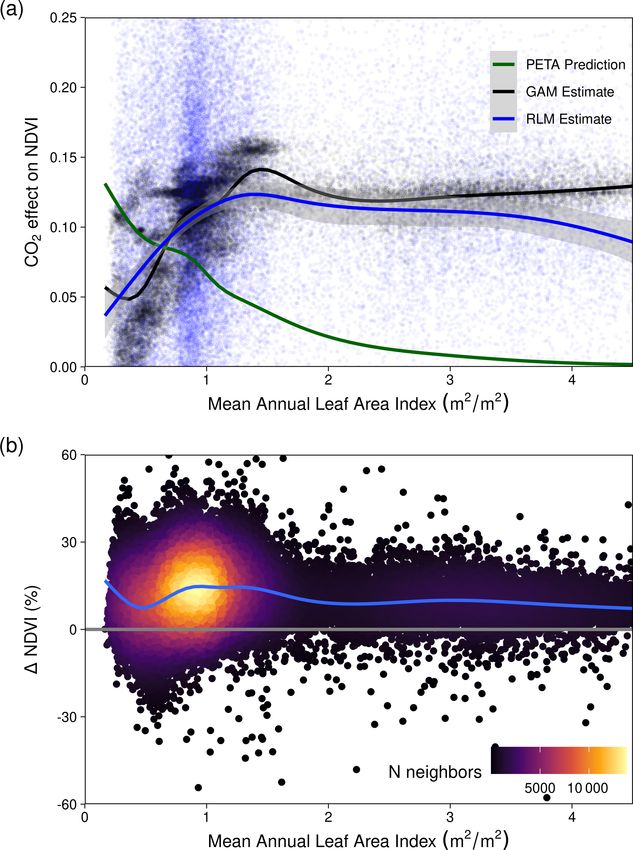
492                                                                                     S. W. Rifai et al.: CO2 -driven greening

centrated in the east, where there are large gradients of pre-      changes in climate, land use, and disturbance are confounded
cipitation (P ) (300–2000+ mm yr−1 ) and potential evapo-           by the effect of CO2 fertilization. Furthermore, the time
transpiration (PET) (800–2100 mm yr−1 ). Most eastern Aus-          series of even the longest systematically collected optical
tralian woodlands occupy water-limited regions where an-            vegetation index records from a single sensor is 20 years
nual PET far exceeds P (Fig. A1 in the Appendix), and tree          (e.g., MODIS Terra). Analysis of trends extending beyond
species have evolved to cope with water-limited conditions          20 years requires merging satellite records across sensors
(Peters et al., 2021) and high interannual rainfall variabil-       and platforms. But this requires care to address changes in
ity. However, the climate is warming: 8 of Australia’s 10           radiometric and spatial resolution of the sensor as well as
warmest years on record have occurred since 2005 (CSIRO             drift in the solar zenith angle (Ji and Brown, 2017; Franken-
and Bureau of Meteorology, 2020), and Australia’s climate           berg et al., 2021) and the time of retrieval. Thus different
has warmed by ∼ 1.5 ◦ C since records began in 1910. The            analytical methodologies have produced disagreements over
warming has likely increased atmospheric demand for water           where greening has occurred (Cortés et al., 2021). One often-
(e.g., PET or vapor pressure deficit, VPD). In most woody           used method to provide additional constraint on greening
ecosystems, the ratio of water supply (i.e., P ) to water de-       trends has been to compare remote-sensing-derived trends
mand (i.e., PET) has declined in recent decades (Figs. 1, 2a).      with modeled changes in leaf area index (LAI) from ensem-
Eastern Australia has also been impacted by several multi-          bles of dynamic global models (Zhu et al., 2016; Wang et al.,
year droughts, episodic deluges of rainfall (King et al., 2020),    2020). However these model attribution approaches rely on
and an increasing frequency of severe heat waves (Perkins           a set of key assumptions. None of the models can accurately
et al., 2012) in the last few decades. Precipitation changes        predict LAI changes in response to rising CO2 (De Kauwe
have been spatially variable over eastern Australia, where          et al., 2014; Medlyn et al., 2016). Vegetation models have
northern Queensland grew wetter, and southeastern Australia         been shown to diverge in their simulation of LAI over Aus-
grew drier (Fig. 2a). In the last 2 decades, southeastern Aus-      tralia (Medlyn et al., 2016; Teckentrup et al., 2021; Zhu et al.,
tralia experienced the two worst droughts in the observa-           2016) and have bioclimatic rules for determining phenology
tional record (2001–2009; van Dijk et al., 2013; and 2017–          which may not be appropriate for the highly variable Aus-
2019; Bureau of Meteorology, 2019). Yet between these               tralian climate and the evergreen Eucalyptus forests (Teck-
two droughts, eastern Australia experienced record-breaking         entrup et al., 2021). These model simulations are typically
rainfall in 2011 associated with a strong La Niña event. This       compared with modeled LAI products derived from the red
caused marked vegetation “greening” (e.g., increased foliar         and near-infrared wavelengths of multispectral satellite sen-
cover), even in the arid interior (Bastos et al., 2013; Poul-       sors, of which each product carries specific algorithmic as-
ter et al., 2014; Ahlstrom et al., 2015). However, this green-      sumptions about canopy-light interception which are condi-
ing contributed to record-breaking fires in the following year      tional upon estimated land cover types. In comparison, NDVI
(Harris et al., 2018).                                              carries no ecosystem-specific assumption and is an effec-
   Theory suggests that plant physiological responses to at-        tive proxy for leaf area in ecosystems with low to moderate
mospheric carbon dioxide (CO2 ) may mitigate some of the            canopy cover (Carlson and Ripley, 1997), a characteristic of
negative effects of an aridifying climate. However, the mag-        eastern Australian woody ecosystems (Specht, 1972; Yang
nitude of plant responses to increased atmospheric CO2 has          et al., 2018).
been challenging to establish in field experiments (Jiang              Here we ask how much greening trends can be explained
et al., 2020b) and from observations (Frankenberg et al.,           by rising CO2 . Using eastern Australia as a model system,
2021; Zhu et al., 2021; Walker et al., 2020) or to sepa-            we used a multi-satellite-derived NDVI record encompass-
rate from other drivers (e.g., climate variability, disturbances,   ing 38 years with multiple statistical techniques to isolate
and changes in land management; Zhu et al., 2016). Studies          the influence of CO2 from simultaneous effects of meteo-
have used data from the Advanced Very High Resolution Ra-           rological change and disturbance. Next we contrasted CO2
diometer (AVHRR) satellites to show positive trends in the          effects with theoretical predictions based on water use effi-
normalized difference vegetation index (NDVI) over Aus-             ciency (WUE) theory for plants and the observed rise in CO2 .
tralia (Donohue et al., 2009). The greening trend is caused         Finally, we examined whether recent NDVI greening trends
by increased leaf area, which has likely resulted from in-          have co-occurred with changes in tree or grass cover over the
creased atmospheric CO2 concentrations (Donohue et al.,             last 2 decades.
2013; Ukkola et al., 2016). The evidence for increases in leaf
area from rising CO2 has also been supported by observa-
tions of reduced runoff in Australia’s drainage basins (Tran-       2     Methods
coso et al., 2017; Ukkola et al., 2016).
   Yet disentangling the CO2 fertilization effect from other        2.1    Study area
drivers of climate variability and global change has been par-
ticularly challenging for satellite-based analyses. It is chal-     The study region encompasses the dominant woody ecosys-
lenging to attribute causes of greening because co-occurring        tems of eastern Australia (Fig. A1b). We used the Na-

Biogeosciences, 19, 491–515, 2022                                                       https://doi.org/10.5194/bg-19-491-2022
S. W. Rifai et al.: CO2 -driven greening                                                                                   493

tional Vegetation Information System 5.1 land cover dataset          We used surface reflectance from two satellite products
(Australian Department of Agriculture, Water and the En-          to generate the NDVI record: National Oceanic and At-
vironment, 2020; Table A1) to select locations desig-             mospheric Administration’s Climate Data Record v5 Ad-
nated as “Acacia Forests and Woodlands”, “Acacia Open             vanced Very High Radiometric Resolution (AVHRR) Sur-
Woodlands”, “Callitris Forests and Woodlands”, “Casuar-           face Reflectance (NOAA-CDR) and the National Aeronau-
ina Forests and Woodlands”, “Eucalypt Low Open Forests”,          tics and Space Administration’s MCD43A4 Nadir Bidi-
“Eucalypt Open Forests”, “Eucalypt Open Woodlands”, “Eu-          rectional Reflectance Distribution Function Adjusted Re-
calypt Tall Open Forests”, “Eucalypt Woodlands”, “Low             flectance (MODIS-MCD43) (Table A1; Schaaf and Wang,
Closed Forests and Tall Closed Shrublands”, “Mallee Open          2015). NDVI data were extracted from 1982–2019 at 0.05◦
Woodlands and Sparse Mallee Shrublands”, “Mallee Wood-            resolution from the NOAA-CDR AVHRR version 5 prod-
lands and Shrublands”, “Melaleuca Forests and Woodlands”,         uct (Vermote and NOAA CDR Program, 2018). The sur-
“Other Forests and Woodlands”, “Other Open Woodlands”,            face reflectance record of AVHRR extends through 2019,
“Rainforests and Vine Thickets”, and “Tropical Eucalypt           but the quality of the record starts to degrade in 2017 be-
Woodlands/Grasslands”.                                            cause of an increase in the solar zenith angle (Ji and Brown,
                                                                  2017), causing a sensor-produced decline in NDVI during
2.2   Climate and remote sensing datasets                         2017–2019. For this reason we only use AVHRR surface re-
                                                                  flectance data between 1982–2016. We composited monthly
We used the atmospheric CO2 record from the deseason-             mean AVHRR NDVI (NDVIAVHRR ) estimates using only
alized Mauna Loa record (https://www.esrl.noaa.gov/gmd/           daily pixel retrievals with no detected cloud cover (qual-
ccgg/trends/data.html, last access: 5 April 2020) and ex-         ity assurance band, bit 1). Monthly NDVIAVHRR estimates
tracted climate data (Table A1) from the Australian Bureau of     aggregated from fewer than three daily retrievals were re-
Meteorology’s Australian Water Availability Project (AWAP;        moved. They were also removed when the coefficient of
Jones et al., 2009). AWAP is a gridded climate product in-        variation in daily retrievals for a given month was greater
terpolated to 0.05◦ from a large network of meteorological        than 25 %. We also removed NDVIAVHRR monthly estimates
stations distributed across Australia. Vapor pressure deficit     where NDVIAVHRR , solar zenith angle, or time of acquisition
was calculated using daily estimates of maximum temper-           deviated beyond 3.5 standard deviations from the monthly
ature and vapor pressure at 15:00 LT (UTC+10). PET was            mean, calculated from a climatology spanning 1982–2016.
calculated from shortwave radiation and mean air tempera-            We used the MODIS-MCD43 surface reflectance at 500 m
ture using the Priestley–Taylor method (Davis et al., 2017).      resolution to derive NDVI for 2001–2019 (NDVIMODIS ).
The Priestley–Taylor method has been shown to be appro-           Monthly mean estimates of the surface reflectance were pro-
priate for estimating large-scale PET (Raupach, 2000) and         duced by compositing pixels flagged as “ideal quality” (qual-
is more suited for use in long-term analysis where CO2            ity assurance, bits 0–1). We also masked disturbances to have
has increased than other common formulations such as the          greater confidence in our attribution of the targeted drivers
Penman–Monteith equation (Greve et al., 2019; Milly and           of NDVIMODIS change (climate and CO2 ). The Global For-
Dunne, 2016), which explicitly imposes a fixed stomatal re-       est Change product v1.7 (Hansen et al., 2013) was used to
sistance that is incompatible with plant physiology theory        mask pixels from 2001 onwards that had experienced for-
(Medlyn et al., 2001). AWAP measurements of shortwave ra-         est loss due to deforestation or severe stand clearing dis-
diation only extend back to 1990, so we extended the PET          turbance. We masked pixel locations that experienced bush-
record to 1982 by calibrating the ERA5-Land PET record            fires from the year 2001 onwards. Specifically, these pix-
(1980–2019) to the AWAP PET record (1990–2019) by lin-            els were masked for the year of burning and the follow-
ear regression for each grid cell and then gap-filled the years   ing 3 years using the 500 m resolution MODIS-MCD64
1982–1989 with the calibrated ERA5 PET. PET from the Cli-         monthly burned-area product (Giglio et al., 2018). We termi-
mate Research Unit record (Harris et al., 2014) was highly        nated the NDVIMODIS time series in August of 2019, prior
correlated with both the recalibrated ERA5 PET (r = 0.91,         to the widespread bushfires of late 2019/early 2020. Both
1982–1989) and the original AWAP PET (r = 0.97, 1990–             NDVIAVHRR and NDVIMODIS datasets were processed using
2019). Next, we calculated a 30-year climatology of the me-       Google Earth Engine (Gorelick et al., 2017) and exported at
teorological variables using the period of 1982–2011 to be        5 km spatial resolution, which best approximated the native
close to current standards (World Meteorological Organiza-        resolution of the NOAA-CDR AVHRR and AWAP products.
tion, 2017). We used this climatology to define the mean an-      Further post-processing used the “stars” (Pebesma, 2020)
nual P : PET (the moisture index, MIMA ) and as the reference     and “data.table” (Dowle and Srinivasan, 2019) R packages
to calculate a 12-month running anomaly of annual P : PET         (see “Code and data availability” section).
(MIanom ). Zonal statistics for each meteorological variable         We merged the processed 1982–2016 NDVIAVHRR with
were calculated using simplified Köppen climate zones, de-        the 2001–2019 NDVIMODIS by recalibrating the NDVIAVHRR
rived from the Australian Bureau of Meteorology (Fig. 2b,         with a generalized additive model (GAM). Specifically, we
Table A1).                                                        used 1 million observations from the overlapping 2001–2016

https://doi.org/10.5194/bg-19-491-2022                                                    Biogeosciences, 19, 491–515, 2022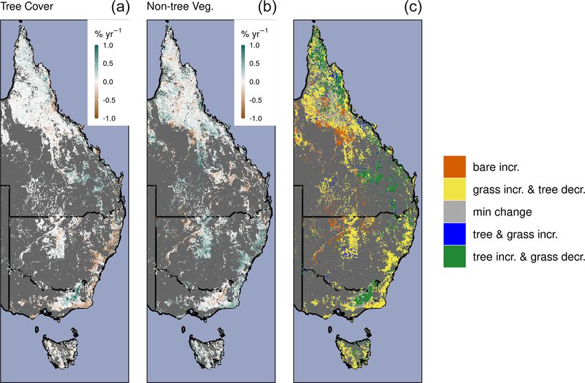
494                                                                                     S. W. Rifai et al.: CO2 -driven greening

portion of both records to fit a GAM using the “mgcv” R             of P : PET was nonlinear and followed a monotonic saturat-
package (Wood, 2017) to model NDVIMODIS from AVHRR-                 ing sigmoidal relationship. GAMs can characterize a nonlin-
derived covariates as                                               ear response without specifying a functional form, yet the
                                                                    underlying spline parameters are not easily interpreted as
NDVIMODIS = s(NDVIAVHRR ) + s(month)                                the parameters of a fixed nonlinear function. Therefore we
             + s(SZA) + s(TOD) + s(x, y),                    (1)    fit models with a set of fixed nonlinear functional forms us-
                                                                    ing nonlinear least squares (nls.multstart package in R v4.01;
where “s” represents a penalized smoothing function using           Padfield and Matheson, 2020) and compared models fit using
a thin plate regression spline; SZA is the solar zenith an-         all pixel locations. The nonlinear functional forms included
gle; NDVIAVHRR is the uncalibrated NDVI from AVHRR;                 the Weibull function (Eq. 4, Fig. 5), the logistic function
TOD is time of day of retrieval; and x and y represent longi-       (Eq. 5, Fig. A5), and the Richards growth function (Eq. 6
tude and latitude, respectively. The fit GAM was then used to       Fig. A6). We focused on the Weibull models because they
generate the recalibrated AVHRR NDVI. The merged NDVI               showed equivalent goodness of fit with fewer parameters
dataset was created by joining the 1982–2000 recalibrated           than the Richards function models. Next we added a linear
AVHRR NDVI with the 2001–2019 NDVIMODIS . We further                modifier to the Weibull function using the covariates of CO2
reduced monthly temporal variability in NDVI by calculating         (µmol µmol−1 ; Ca ) and the ratio of the anomaly of P : PET
a 3-month rolling mean of NDVI, which we used for subse-            (MIanom ) to the mean annual P : PET (MIMA ) as follows:
quent statistical model fitting.
                                                                    NDVI = Va − Vd [exp(− exp(cln ) (MIMA )q )] + η
2.3   Estimating NDVI and climate trends                                   MIanom                       MIanom
                                                                    η = β1        + β2 Ca MIMA + β3 Ca            + sensor.     (4)
                                                                           MIMA                         MIMA
We estimated the relative increase in NDVI between 1982–
                                                                    Here the sensor term is a binary covariate indicating the
2019 with respect to time (Eq. 2) for each grid cell with an
                                                                    AVHRR or MODIS sensor. Model-fitted parameters Va and
iteratively weighted least squares robust linear model via the
                                                                    Vd correspond to the asymptote and the asymptote’s differ-
“rlm” function in R’s MASS package (Venables and Ripley,
                                                                    ence from the minimum NDVI, while cln is the logarithm of
2002) as follows.
                                                                    the rate constant, and q is the power to which MIMA is raised.
                                                                    The model was fit by individual season with 1 million obser-
NDVI = β0 + β1 year + β2 sensor                              (2)
                                                                    vations per model fit. Corresponding goodness-of-fit metrics
Here β0 represents the estimated NDVI in 1982, the year             (R 2 and root mean square error) were calculated by season
term starts at 1982, and the sensor term is a binary covariate      (Fig. 5) with 1 million randomly sampled observations.
that accounts for residual offset differences between the re-           We tested alternative nonlinear functional forms to char-
calibrated AVHRR NDVI and the NDVIMODIS . The relative              acterize the effect of CO2 upon NDVI. A logistic model was
temporal trends for climate variables and the MODIS vege-           fit across space for each hydrological year as
tation continuous fractions were fit for each grid cell location                         VA
using the Theil–Sen estimator, a form of robust pairwise re-        NDVI =                                ,                     (5)
                                                                              (1 + exp((m − MI12 mo )/s))
gression, with the “zyp” R package (Bronaugh and Werner,
2019). The temporal covariate was recentered to start with          where NDVI is the hydrological year mean value of NDVI
the first hydrological year (where the year starts 1 month ear-     for a grid cell location, m is the midpoint, s is a scale param-
lier in December) of the data so that the intercept term repre-     eter, and VA is the asymptote (plotted in Fig. A5). We also
sents the mean at the start of the time series. The relative rate   used a modified Richards growth function to characterize the
of change for each variable was reconstructed by calculating        CO2 effect upon seasonal NDVI (Fig. A6) as
                                                                  NDVI = (VA + β1 Ca + β2 MIf.anom )
         β1 (yearend − yearstart )
100 ·                                ,                        (3)          (1 + exp(m + β3 Ca + β4 MIf.anom − MIMA ))
                   β0                                                   ·
                                                                         (s + β5 Ca + β6 MIf.anom )(− exp(−(q+β7 Ca +β8 F )))
where β0 and β1 are the intercept and trend derived from                        MIanom
Theil–Sen regression.                                               MIf.anom =         .                                        (6)
                                                                                 MIMA
2.4   Estimating contribution of CO2 and climate                    Here the β terms act to linearly modify the core nonlinear pa-
      toward NDVI trends                                            rameters (VA , m, s, q) with the effects of CO2 and MIf.anom .
                                                                    Each seasonal model component was fit across space with 1
We fit six forms of statistical models to the merged NDVI           million random samples from the total merged NDVI record
observations in order to quantify the impact of changes in          (approximately 14.3 million observations).
CO2 and meteorological variables on NDVI. Figure 1 shows              To ensure consistent interpretation of the nonlinear re-
that the relationship between NDVI and multi-annual mean            sponse across P : PET, we also fit linear models explaining

Biogeosciences, 19, 491–515, 2022                                                       https://doi.org/10.5194/bg-19-491-2022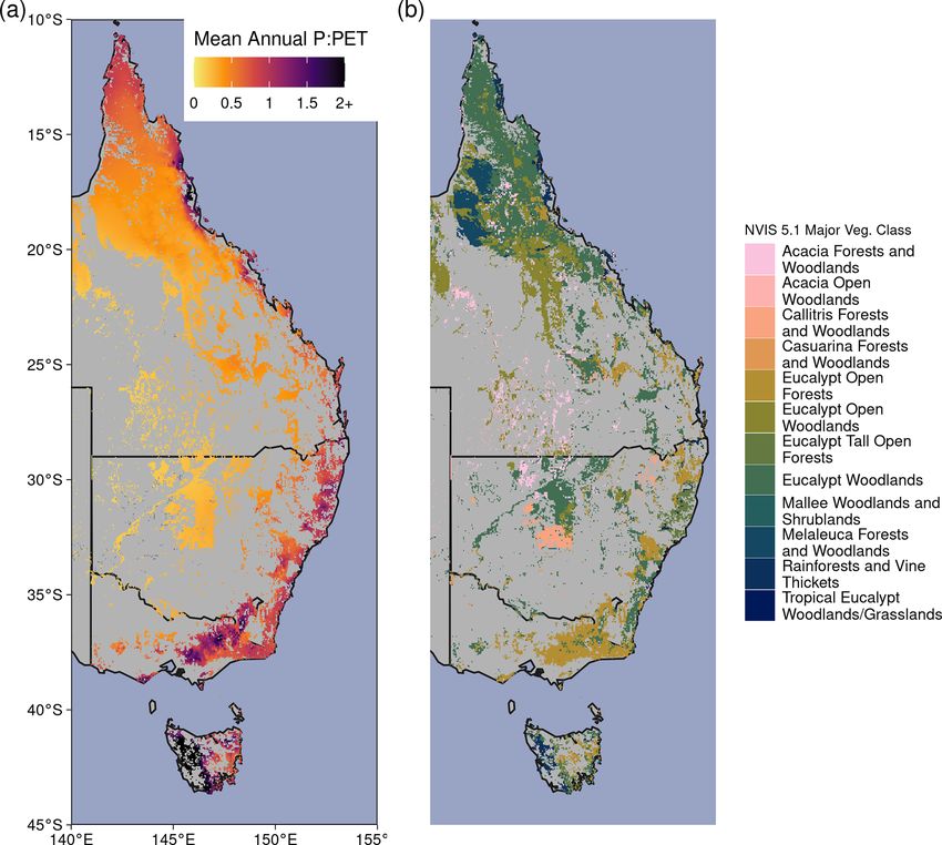
S. W. Rifai et al.: CO2 -driven greening                                                                                     495

NDVI with CO2 and MIanom by season in MIMA bin widths              (mol mol−1 ). The relative rate of change in W with respect
of 0.2 (Eq. 7, Fig. A4). Separate linear models were fit for in-   to a change in Ca can be calculated as
crements of 0.15 of MIMA for each season using the merged
                                                                   dWleaf   dAleaf dEleaf   dCa dD d(1 − χ )
1982–2019 NDVI record. NDVI was modeled as                                =       −       =    −   +          .             (11)
                                                                    Wleaf   Aleaf   Eleaf   Ca   D   (1 − χ )
NDVI = β0 + β1 Ca + β2 MIanom + β3 Veg. Class
                                                                   If temperature increases without a corresponding increase in
      + β4 sensor,                                          (7)    humidity, D increases, which also causes transpiration to rise
                                                                   and thus reduces W . However, W is predicted to increase
where Veg. Class is the NVIS 5.1 vegetation class, and sensor
                                                                   with CO2 , which may offset increases in D. Experiments
is a binary variable used to account for residual differences
                                                                   suggest that χ does not change with Ca but is sensitive to D
between the recalibrated AVHRR NDVI and NDVIMODIS
                                                                   (Wong et al., 1985; Drake et al., 1997) and can be estimated
records. To aid the comparison of model effects, we centered
                                                                   as being proportional to the square
                                                                                                    √ root of D (Medlyn et al.,
and standardized the continuous model covariates before re-
                                                                   2011). By substituting 1 − χ ≈ (D) into Eq. (11) we can
gression. The standardized CO2 and P : PETanom effects (β)
                                                                   estimate the theoretical combined effect of Ca and D upon
are presented in Fig. A4.
                                                                   Wleaf as
   Next, to produce spatially varying estimates of the CO2
effect, we fit robust multiple linear regression models to         dWleaf   dAleaf dEleaf   dCa 1 dD
the time series of NDVI for each of the 39 463 pixel loca-                =       −       =    −     .                      (12)
                                                                    Wleaf   Aleaf   Eleaf   Ca   2 D
tions. The CO2 effect for each grid cell location was simul-
taneously estimated with the linear effects of the anomalies          Transpiration per unit ground area is strongly con-
(anom) of P , PET, VPD, and MI as fractions of their mean          trolled by water supply in warm, water-limited environ-
annual (MA) values as follows:                                     ments with relatively low leaf area such as eastern Australia
                                                                   (Specht, 1972); therefore we approximate canopy transpira-
                           Panom      PETanom                      tion (Ecanopy ) as
NDVI = β0 + β1 Ca + β2           + β3
                           PMA        PETMA
             VPDanom                                               Ecanopy = Eleaf L,                                       (13)
      + β4           + β5 sensor.                           (8)
             VPDMA                                                 where L is leaf area. The change in Ecanopy can then be de-
Finally we produced a GAM to estimate the CO2 effect in            fined as
addition to the nonlinear interactions between CO2 , mean          dEcanopy   dEleaf dL
annual climate, and climate anomalies. Here instead of pre-                 ≈       +   .                                   (14)
                                                                    Ecanopy   Eleaf   L
determined nonlinear functional forms, the GAM used pe-
nalized smoothing functions (s) to estimate the potentially           If we assume there is no overall change in precipitation
nonlinear effect of the covariates. The GAM was fit across         then we can assume change in Ecanopy is tightly coupled to
all pixel locations and estimated the CO2 effect and the ef-       the water supply; therefore we have
fects of the anomalies and mean annual values of VPD, P ,
                                                                       dEleaf   dL
and PET as well as sensor epoch as follows:                        −          ≈    .                                        (15)
                                                                        Eleaf   L
NDVI = s(MIMA , Ca ) + s(VPDanom , VPDMA )                         We note that the assumption of constant precipitation is obvi-
      + s(Panom , PMA ) + s(PETanom , PETMA ) + sensor.            ously unrealistic, most notably because two major droughts
                                                            (9)    occurred during the observation period. However, over much
                                                                   longer periods (i.e., 1910–2018) precipitation in eastern Aus-
2.5   A simplified theoretical water use efficiency model          tralia has been relatively stationary (Ukkola et al., 2019).
                                                                      NDVI is linearly related to foliar cover (F ) until LAI ≈ 3
We compared the statistically attributed CO2 amplification of      (m2 m−2 ) (Carlson and Ripley, 1997), which is predomi-
NDVI with the expectation from a simple theoretical model          nantly the case when P : PET < 1. Most woody ecosystems
of WUE. Following Donohue et al. (2013), WUE (W ) is de-           in eastern Australia are strongly water-limited with LAI ≤ 1
fined as                                                           (m2 m−2 ), where NDVI is approximately proportional to the
                                                                   fraction of foliar cover:
          Aleaf    Ca
Wleaf =         =      (1 − χ ),                           (10)    dL dF    dNDVI
          Eleaf   1.6D                                                ≈   ≈       .                                         (16)
                                                                    L   F    NDVI
where A is leaf-level carbon assimilation    (µmol m2 s−1 ),
                                                           E
                                                                   Then substituting Eq. (15) into Eq. (12) gives
is leaf-level transpiration (µmol m2 s−1 ), Ca is atmospheric
CO2 (µmol µmol−1 ), Ci is intercellular CO2 (µmol µmol−1 ),        dWleaf   dAleaf dF   dCa 1 dD
χ is CCai , and D is atmospheric vapor pressure deficit                   ≈       +   ≈     −     .                         (17)
                                                                    Wleaf   Aleaf   F    Ca   2 D

https://doi.org/10.5194/bg-19-491-2022                                                      Biogeosciences, 19, 491–515, 2022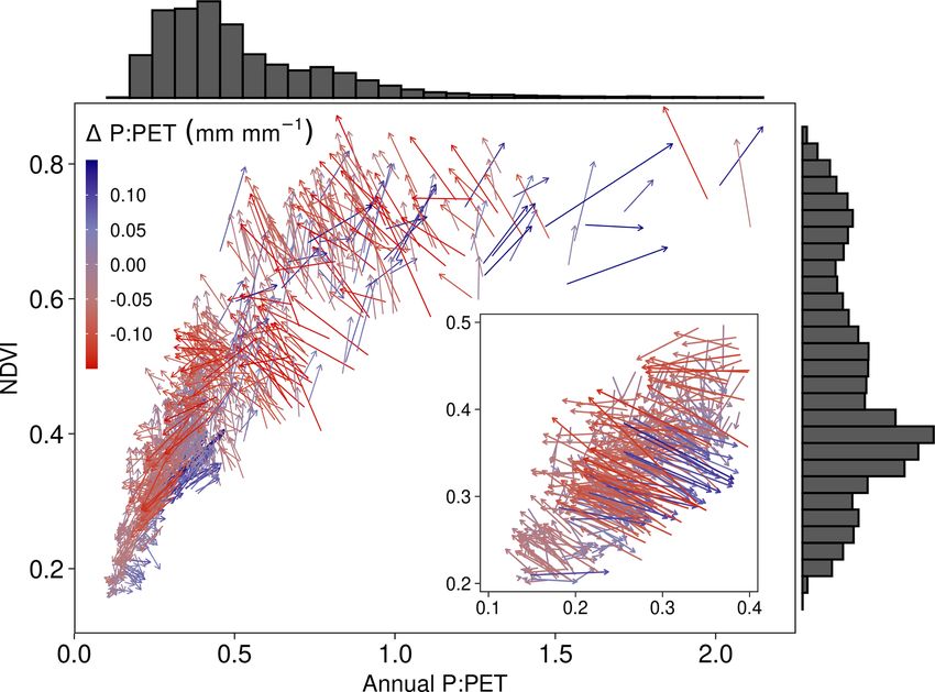
496                                                                                        S. W. Rifai et al.: CO2 -driven greening

Figure 1. Individual grid cell temporal 38-year trajectories of the
normalized difference vegetation index (NDVI) and the ratio of
annual precipitation (P ) to potential evapotranspiration (PET). A
vector field plot showing the direction of change in mean annual
NDVI and P : PET between 1982–1986 and 2015–2019 for 1000
randomly sampled grid cell locations (color indicates direction of
change in P : PET as indicated by legend). An inset shows a mag-
nification of the samples from the 0.1–0.4 P : PET range. The dis-
tributions of mean P : PET (mm mm−1 ) and NDVI for the period
of 1982–1986 are shown as histograms above and to the right of the
main panel. Note that the majority of arrows shift towards higher     Figure 2. Long-term aridity change and climate zones. (a) The lin-
aridity (lower P : PET) and higher NDVI.                              ear trend of annual P : PET (the moisture index) between 1982–
                                                                      2019, (b) simplified Köppen climate zones. Climate zone abbrevia-
                                                                      tions correspond to Equatorial (Equat.), Tropical (Trop.), Subtropi-
   If we assume that the benefit towards Wleaf from rising Ca         cal (Subtr.), Grassland (Grass.), Temperate (Temp.), and Temperate
is split evenly between the relative changes in Aleaf and F ,         Tasmania (Tasm.).
we can predict the change towards NDVI to be

dNDVI 1 dCa dD                                                        3     Results
      ≈      −      .                                         (18)
 NDVI   2 Ca   2D
                                                                      3.1    Long-term greening in a changing climate
   We compared the WUE theoretical model with the robust
linear models fit for each pixel location (Eq. 8) and the GAM         Parts of northern Queensland grew wetter, but aridity (as
(Eq. 9) fit across the study region. The WUE theoretical              measured by reduced P : PET) increased in over 52 % of
model assumes no change in P but does account for changes             eastern Australian woody ecosystems since 1982 (Figs. 1,
in VPD. Therefore in using the statistical models to com-             2a). Aridity decreased over northern Queensland, encom-
pare with the WUE predictions, we generated counterfactual            passing the entirety of Equatorial and Tropical regions
predictions from the statistical models with no precipitation         and most of the Grassland and Subtropical regions, driven
anomaly but with the observed increases in CO2 and VPD.               by large wet-season increases in precipitation (Fig. A2a).
One weakness with the application of this WUE theoretical             Widespread increases in PET were evident from September–
model is the uncertainty regarding the assumed allocation of          February (Fig. A2b). At the same time as these changes in
the Wleaf benefit towards either Aleaf or F (e.g., LAI; see           climate were occurring, over 92 % of these regions expe-
above). Donohue et al. (2017) proposed a similar model to             rienced overall greening (Fig. 3a), including regions where
Eq. (18), the partitioning of equilibrium transpiration and as-       P : PET declined (Figs. 1, 2b, A3). The relative increases in
similation (PETA) hypothesis, where the relative allocation           NDVI were comparable between the earlier AVHRR epoch
to leaf area is predicted to decline with increasing resource         (1982–2000) and the later MODIS epoch (2001–2019) at
availability (which could be inferred from growing season             5.7 % (CI = [−2.9 %, +20.3 %]) and 5.1 % (CI = [−6.4 %,
LAI). We calculated the expectation from the PETA hypoth-             +20.1 %]), respectively. However, the spatial patterns of
esis as another point of comparison with the CO2 -attributable        greening and/or browning differed between epochs (Fig. 3b),
effect on NDVI.                                                       and most regions also showed high decadal-scale variabil-

Biogeosciences, 19, 491–515, 2022                                                          https://doi.org/10.5194/bg-19-491-2022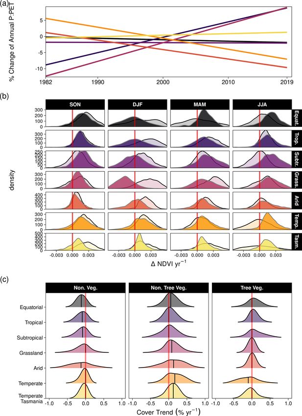
S. W. Rifai et al.: CO2 -driven greening                                                                                      497

ity in greening and/or browning trends (Fig. 4). The overall      3.3   CO2 -driven greening and expectations from water
greening trends between the AVHRR 1982–2000 epoch and                   use efficiency
the MODIS 2001–2019 epoch generally agree across regions
and seasons. However linear NDVI trends fit over shorter in-      The range of statistically estimated CO2 -attributable green-
tervals of 10 years are much less consistent (Fig. 4), exempli-   ing responses were compared with the expectation from the
fying the importance of estimating trends over long enough        theoretical CO2 water use efficiency model. The Donohue et
periods to average over decadal-scale variability. Long-term      al. (2013) CO2 ×WUE model (see “Methods”) accounts for
browning only occurred in the Arid region (Figs. 3, 4). Nev-      changes in VPD but assumes no change in water supply. As-
ertheless, by examining NDVI trends over nearly 40 years,         suming an equal split in the benefits of WUE between greater
we were able to separate regional decadal-scale variability       carbon assimilation and increased foliage cover (see below
from the overall broad greening trend across eastern Aus-         for alternative assumptions), the model predicted an 8.7 %
tralia (Figs. 3, 4, A3).                                          (10th–90th percentile range [+6.8 %, +10.2 %]) increase in
                                                                  NDVI (proxy for foliage cover; see “Methods”). This com-
3.2   Empirical attribution of the CO2 effect                     pared to an estimated 11.7 % ([+4.6 %, +14.6 %]) relative
                                                                  increase from the GAM when accounting for a simultaneous
                                                                  increase in VPD (which the WUE accounts for) and factor-
We found consistently positive NDVI responses to CO2              ing out the effects of changing precipitation and PET (which
across the moisture gradient of P : PET for all seasons, with     the WUE model does not account for). We needed to assume
the greatest increases located in regions of higher P : PET       differing levels of allocation to foliar gain (i.e., not 50 %)
(> 0.5) (Fig. 5). The nonlinear Weibull models showed a           for the theoretical WUE model to match the statistically
larger CO2 -attributable effect on NDVI in regions of higher      estimated CO2 effect (Fig. 7e). Regions of higher P : PET
P : PET (Fig. 5), but the effect size of the NDVI response to     (Equatorial, Tropical, Temperate, and Temperate Tasmanian)
CO2 was largely consistent across model forms (Figs. A4–          required greater allocation fractions than 50 %, whereas the
A7). The CO2 -attributable increase in NDVI between 1982–         allocation fraction would be between 25 %–50 % for regions
2019 ranged from approximately 5 % in the Arid interior re-       with lower P : PET (Arid, Grassland, and Subtropical). In
gions to > 20 % in the wettest Tropical and Temperate re-         comparison, the PETA hypothesis (Donohue et al., 2017)
gions (Fig. 5a). This was consistent with linear model forms      predicted the greatest CO2 effect on leaf area to be in regions
when fit for individual grid cell locations (Eq. 8, Fig. 6) as    with the lowest LAI, but this was not supported by the sta-
well as by comparing the CO2 effect size across 16 linear         tistically estimated CO2 effect on NDVI (Fig. A9). Despite
models fit for grid cell locations grouped into bins spanning     having the lowest LAI, the Arid region received the smallest
0.1 increments of P : PET (Eq. 7, Fig. A4). The GAM fit           CO2 effect, but it is worth noting that the Arid region also
across grid cell locations also indicated a larger CO2 effect     experienced the greatest increase in VPD and reduction in P
in regions with higher P : PET (Figs. 6, 7b). Quantile regres-    over the 38-year period (Figs. 7a, A8). In contrast, the largest
sion with generalized additive models showed a pronounced         estimated CO2 -attributable effects on greening were found to
response to CO2 across the distribution of pixels with both       be in the Equatorial and Tropical areas.
low and high NDVI (10–97.5 percentiles) across the full arid-
ity gradient of P : PET (Fig. A7).
   A recent study found that the global CO2 fertilization ef-     3.4   Co-occurring shifts in aridity, NDVI, and
fect was halved between the 1980s and 2000s (Wang et al.,               vegetation cover
2020). In contrast to the estimates over eastern Australia
from Wang et al. (2020), we found no consistent evidence          The shifts in P : PET and NDVI were accompanied by vege-
of a decline in the effect of CO2 on NDVI through time.           tation cover changes in some regions. Most notably, the Arid
Neither the GAM estimates nor the robust linear model es-         and Temperate regions experienced the strongest zonally av-
timates of the CO2 effect showed any consistent evidence of       eraged declines in P : PET (Fig. 8a) and increases in VPD
a weakening CO2 effect between 1982–2000 and 2001–2019            (Fig. A8). Seasonal greening trends were relatively simi-
(Fig. 6). The central 25th–75th percentiles of the distribu-      lar apart from the aforementioned exceptions in the Grass-
tion of robust linear model effect sizes overlapped in all re-    land. The MODIS vegetation continuous fraction data from
gions between epochs. The central 25th–75th percentiles of        2001–2018 indicated that most regions experienced modest
the GAM-estimated distributions also overlapped, with the         changes in tree vegetation cover. The largest decline in tree
exception of the Grassland and Arid regions, where the CO2        cover occurred in the Temperate regions (Figs. 8c, A10).
effect was larger during 2001–2019. Consistent with the find-     Most regions experienced declines in non-vegetated (bare)
ing of a greater CO2 effect in wetter regions (Fig. 5), the ro-   cover, increases in non-tree vegetation, and modest change
bust linear models and the GAM estimated the CO2 effect to        in tree cover (Fig. 8c); however the proportional increase in
be greatest in the Equatorial and Tropical regions and lowest     non-tree vegetation typically exceeded tree cover increases
in the Arid region (Fig. 6).                                      (Fig. A10).

https://doi.org/10.5194/bg-19-491-2022                                                      Biogeosciences, 19, 491–515, 2022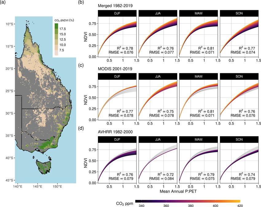
498 S. W. Rifai et al.: CO2 -driven greening
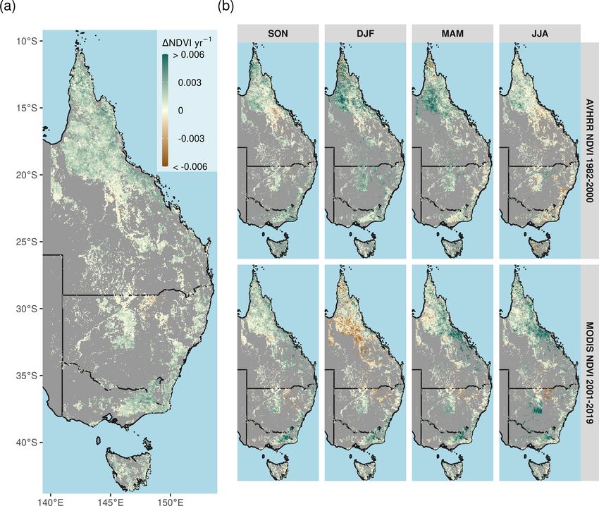
Figure 3. Overall long-term NDVI change and change shown by satellite epoch and season. (a) The annual rate of NDVI change from the
merged satellite record spanning 1982–2019. The seasonal AVHRR NDVI between 1982–2000 (b, top row) and MODIS NDVI between
2001–2019 (b, bottom row). Non-woody ecosystem regions are masked in gray. A notable browning trend is evident at the interface of the
Grassland and Arid regions during DJF of the MODIS time period. Note: season abbreviations correspond to September–October (SON),
December–February (DJF), March–May (MAM), and July–August (JJA).
4 Discussion Prior global analyses on warm arid environments have
quantified the CO2 effect on greening (Donohue et al.,
4.1 Australian woody vegetation as model systems to 2013). More expansive global-scale analyses of all terres-
quantify CO2 fertilization trial vegetation using dynamic global vegetation model at-
tribution have found evidence to connect Australia’s green-
Australia is ideal to explore the CO2 contribution towards ing to changes in atmospheric CO2 concentration (Winkler
vegetation greening because there are fewer confounding ef- et al., 2021), while an earlier study did not (Zhu et al., 2016).
fects to drive greening. Forest trees are evergreen, and the Australian studies documented the greening trend up to 2010
growing season is rarely limited by temperature or radiation. using the long-term AVHRR record (Donohue et al., 2009;
The study region spans a large moisture gradient (Fig. A1a), Ukkola et al., 2016) and have been able to partially attribute
but unlike much of the global tropics, the large majority CO2 as a driver of greening in sub-humid and semi-arid re-
of the study region is not so cloudy as to prevent multiple gions. Here we advanced upon prior research to separate the
high-quality multispectral satellite retrievals per month. Aus- effects of disturbance and changes in aridity and moisture in
tralia has also not been subjected to other prominent drivers order to quantify the CO2 fertilization effect across the full
of greening such as nitrogen deposition (Ackerman et al., spectrum of moisture availability experienced by Australian
2019). Nevertheless, Australia has experienced notable land woody ecosystems, notably for 38 years.
use change during the study period such as high rates of de-
forestation in Queensland and northern New South Wales
(Evans, 2016). However, we excluded affected pixel loca-
tions from the analysis.
Biogeosciences, 19, 491–515, 2022 https://doi.org/10.5194/bg-19-491-2022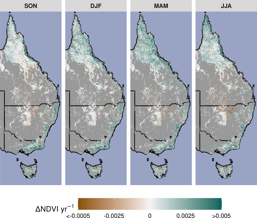
S. W. Rifai et al.: CO2 -driven greening                                                                                               499

Figure 4. Variability in linear trends over varying time periods by season and climate zone. The black line represents the overall 1982–
2019 trend, the light-green line represents the calibrated 1982–2000 AVHRR, and the green line represents the 2001–2019 MODIS. Gray
colors indicate linear trends from overlapping 10-year time intervals. The boundaries of the climate zones are shown in Fig. 2b. Note:
climate zone abbreviations correspond to Equatorial (Equat.), Tropical (Trop.), Subtropical (Subtr.), Grassland (Grass.), Temperate (Temp.),
and Temperate Tasmania (Tasm.). Season abbreviations correspond to September–October (SON), December–February (DJF), March–May
(MAM), and July–August (JJA).

4.2   Regional differences in greening and browning                     more than half of the Equatorial, Tropical, Subtropical, and
      through time                                                      Grassland regions in northern Queensland experienced in-
                                                                        creases in precipitation since 1982 (Fig. A2; Ukkola et al.,
Despite the region’s high decadal-scale variability in NDVI             2019), thus allowing these locations to exceed the predicted
(Fig. 4), the nearly 4-decade-long record allowed us to sep-            NDVI increases from the WUE model (Fig. 7d).
arate the CO2 effect on NDVI from the anomalies caused                     It should be noted that not all regions experienced consis-
by drought (e.g., 2003–2009) or high rainfall (e.g., La Niña            tent greening trends throughout the observation period. For
2010–2011). Although the long-term greening trends we                   example, “greening” shifted to “browning” during the austral
document in the 9 years following earlier studies are gen-              summer (December–February) in the Arid and Grassland re-
erally consistent (Donohue et al., 2009; Ukkola et al., 2016),          gions of Queensland between the 1982–2000 and 2001–2019
our results diverge and lead to key differences in interpreta-          records (Fig. 3b). It is unclear why browning occurred during
tion of why NDVI has continued to increase. First, while the            austral summertime in the Grassland region (Figs. 3b, 4, 8b).
relative increases in NDVI between the 1982–2000 AVHRR                  The declines in NDVI during 2001–2019 may have been me-
epoch (5.7 %) and the 2001–2019 MODIS epoch (5.1 %) are                 teorologically driven and related to shifts in the distribution
comparable (Figs. 3b, 8b), the underlying reasons for the               of wet- and dry-season precipitation (Fig. A2). Alternatively,
change differ. VPD changed minimally between 1982–2000,                 the shift could be due to changes in fire and cattle manage-
whereas it rapidly increased between 2001–2019 (Fig. A8).               ment that have been particularly prevalent across regions of
These increases were largest in the most Arid and Temperate             Queensland in recent decades (Seabrook et al., 2006). Fur-
regions (12.7 % and 11 % since 1982, respectively; Fig. 6),             ther, greening may have been suppressed in parts of Queens-
and when coupled with seasonal reductions in precipitation              land because cattle ranching activity has intensified and has
(Fig. A2) these would have partially offset benefits from in-
creased intrinsic water use efficiency (Eq. 17). In contrast,

https://doi.org/10.5194/bg-19-491-2022                                                              Biogeosciences, 19, 491–515, 2022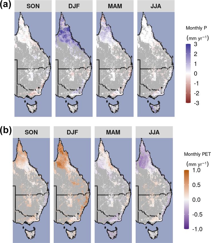
500                                                                                           S. W. Rifai et al.: CO2 -driven greening

Figure 5. Effect of increasing CO2 on seasonal NDVI across P : PET. Predictions of seasonal NDVI as a function of mean annual P : PET fit
using a standard Weibull function (see “Methods”, Eq. 2), modified with linear effects of CO2 , the running 12-month anomaly of P : PET, and
the satellite sensor. The CO2 concentration gradient represents the atmospheric CO2 change between 1982–2019. Panel (a) maps the total
predicted contribution of CO2 towards the relative increase in NDVI between 1982–2019 assuming no anomaly of P : PET. Panel (b) shows
the merged sensor response between 1982–2019 across the gradient of mean annual P : PET, (c) shows the model response when fit using just
MODIS MCD43 data between 2001–2019, and (d) shows the response when the model was fit with the recalibrated AVHRR data between
1982–2000. The AVHRR- and MODIS-satellite-epoch NDVI predictions are plotted in gray for (b) and (c), respectively.

driven forest conversion to managed pasture in the region               found weakening of the CO2 fertilization effect across both
(McAlpine et al., 2009).                                                southeastern and northern Australia (Wang et al., 2020). We
                                                                        found no meaningful difference in the CO2 -attributable ef-
4.3   Attributing a CO2 fertilization contribution                      fect towards greening between the AVHRR 1982–2000 and
      towards greening                                                  MODIS 2001–2019 epochs to support the finding of a tem-
                                                                        porally weakening CO2 effect (Fig. 6). The WUE model
                                                                        predicted similar relative rates of NDVI increase between
Plants increase their rates of photosynthesis in response to
                                                                        the two epochs (4.5 % and 4.7 % for AVHRR and MODIS),
rising atmospheric CO2 whilst also reducing stomatal con-
                                                                        yet for different reasons. CO2 increased by 30 ppm between
ductance, which reduces evaporative losses, and combined,
                                                                        1982–2000, while VPD changed minimally, and precipita-
the two responses lead to greater WUE (Ainsworth and
                                                                        tion increased in Queensland and the Arid region (Fig. A8),
Rogers, 2007; Morison, 1985). In water-limited ecosystems,
                                                                        all of which are favorable to increasing NDVI. In contrast,
it has been hypothesized that this physiological response by
                                                                        the larger CO2 increase between 2001–2019 (40 ppm) was
plants to CO2 should result in increased leaf biomass (Dono-
                                                                        offset by a spatially ubiquitous increase in VPD (3.7 %,
hue et al., 2013; Ukkola et al., 2016). While all of our statis-
                                                                        CI = [−0.4 %, 8.6 %]; Fig. A8) and the occurrence of two
tical approaches indicated a year-round positive CO2 effect,
                                                                        multi-year droughts (Millennium Drought, 2003–2009, and
in contrast to theory the effect was consistently greater in
                                                                        The Big Dry, 2017–2020). Despite the widespread evidence
regions with higher P : PET (Figs. 5–7, A4–A7). Our anal-
ysis also diverges with a global coarse-scale analysis that

Biogeosciences, 19, 491–515, 2022                                                             https://doi.org/10.5194/bg-19-491-2022
S. W. Rifai et al.: CO2 -driven greening 501
Figure 6. Boxplot representation of the CO2 -attributable effect upon changing NDVI. Here the 25th, 50th, and 75th percentiles of the CO2 -
attributable effect on NDVI are shown. The robust linear models (RLM; see “Methods”, Eq. 13) were fit for each individual grid cell location,
whereas the generalized additive model (GAM; see “Methods”, Eq. 14) was fit using all grid cell locations. The distribution of RLMs yielded
a median R 2 of 0.58 and RMSE of 0.025 over the merged period. The GAM had an overall R 2 of 0.91 and RMSE of 0.049.
of the CO2 effect, the WUE model notably underpredicted the course of the study (Fig. A2), and this higher concentra-
greening in some regions (Fig. 7). tion of rainfall during the warmest months is thought to favor
C4 grasses (Hattersley, 1983; Knapp et al., 2020; Murphy
4.4 Deviations from WUE and Bowman, 2007). Finally, the linear dependency of leaf
area upon VPD in the theoretical model may be ill-suited for
We found that the CO2 effect on foliar area was the small- extreme anomalously arid conditions because NDVI obser-
est in the driest climate regions (Figs. 5–6, A4–A7). This vations suggest a strongly nonlinear relationship with large
was at odds with the WUE prediction (at 50 % allocation; VPD anomalies (Fig. A11).
Fig. 7e) and contrary to the expectation that the greatest We explored how much of the higher WUE benefit would
WUE-derived benefit from CO2 would be in drier climates have to be allocated to match the GAM-estimated CO2 -
(Donohue et al., 2017; McMurtrie et al., 2008). These devi- attributed changes in NDVI. Allocation rates far greater than
ations may have resulted from ecosystems processes beyond 50 % would be required to match the WUE prediction in the
the scope of a simple model, such as more severe nutrient Tropical and Equatorial zones (Fig. 7e), whereas allocation
limitations, the phenology of the vegetation composition, be- would need to be less than 50 % to match the GAM esti-
lowground root processes, and disturbances not captured by mate in the Arid region. The Arid region experienced the
the satellite products (e.g., small fires, grazing). Browning in greatest relative increase in VPD (Figs. 7a, A8), yet the the-
the Grassland region (Figs. 3b, A3) may have been caused by oretical model still predicted a small but positive increase in
distinct dry-season phenological differences between over- NDVI (Fig. 7c), which the GAM estimate suggests would
story woody vegetation and understory C4 grasses (Moore be closer to a 10 % rather than 50 % foliar allocation level
et al., 2016), which are dominant there (Murphy and Bow- from the WUE benefit (Fig. 7d). Nevertheless, the smaller
man, 2007). C4 grasses may have been favored over C3 be- effect over the Arid region was consistent with earlier obser-
cause precipitation increased during the austral summer over vational findings across Australia (Ukkola et al., 2016) and
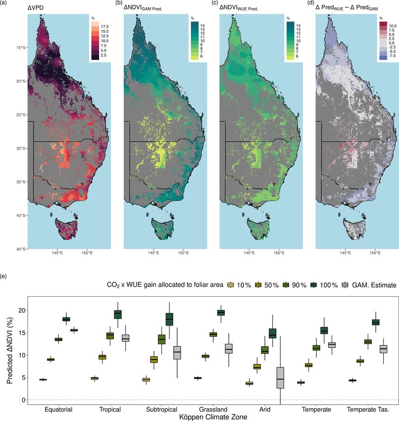
https://doi.org/10.5194/bg-19-491-2022 Biogeosciences, 19, 491–515, 2022502 S. W. Rifai et al.: CO2 -driven greening Figure 7. Long-term changes in vapor pressure deficit and comparison between the 1NDVI due to CO2 and the expected CO2 fertilization effect on foliar area due to gains in water use efficiency (WUE). (a) The relative increase in the annual mean of vapor pressure deficit (VPD) between 1982–2019. (b) The predicted relative increase in NDVI due to CO2 (see “Methods”, Eq. 14) with a concurrent increase in VPD. (c) The relative expected increase in NDVI following the theoretical WUE prediction where 50 % of the gain is allocated to foliar area (see “Methods”, Eq. 11). (d) The difference between the predictions of relative NDVI from the WUE model with 50 % allocation and the GAM-estimated relative increase caused by CO2 . Blue regions indicate where the GAM prediction was greater than the WUE prediction. (e) Boxplot of the expected relative NDVI % increase from WUE gains due to CO2 fertilization depending upon differing levels of foliar allocation from the CO2 benefit toward WUE and the GAM-estimated NDVI% increase due to CO2 (see “Methods”, Eq. 11). The boxplot distribution of the Equatorial region appears collapsed because the Equatorial portion of the region is relatively small (a). Biogeosciences, 19, 491–515, 2022 https://doi.org/10.5194/bg-19-491-2022
S. W. Rifai et al.: CO2 -driven greening                                                                                               503

Figure 8. The relative percentage change in P : PET by climate zone and corresponding distributions of 1NDVI yr−1 and percentage
annual change in vegetation cover fraction. (a) The linear relative changes in annual P : PET trend by climate zone between 1982–2019,
as estimated by robust regression (see “Methods”). The annual P : PET change (%) and corresponding standard error were as follows:
Equatorial (−0.045 ± 0.01), Tropical (0.477 ± 0.005), Subtropical (−0.007 ± 0.005), Grassland (0.576 ± 0.006), Arid (−0.293 ± 0.006),
Temperate (−0.342 ± 0.004), and Temperate Tasmania (0.047 ± 0.005). (b) Distribution of linear long-term NDVI trends for the six climate
clusters by season using the Theil–Sen estimator. Filled distributions are trends from the MODIS sensors (2001–2019), and transparent
(black outline) distributions are from the AVHRR sensors (1982–2000). (c) Distributions of the linear pixel-level trends using the Theil–Sen
estimator for non-vegetated cover, non-tree vegetation cover, and tree cover between 2000–2018. The median is overlaid. Note that climate
zone abbreviations are as follows: Equatorial (Equat.), Tropical (Trop.), Subtropical (Subtr.), Grassland (Grass.), Temperate (Temp.), and
Temperate Tasmania (Tasm.).

https://doi.org/10.5194/bg-19-491-2022                                                              Biogeosciences, 19, 491–515, 2022
504                                                                                    S. W. Rifai et al.: CO2 -driven greening

experimentation from the Nevada Desert FACE experiment             (Atlas of Living Australia, 2020). Similarly, a study using an
(Smith et al., 2014).                                              experimental constrained plant hydraulics model to predict
                                                                   the regions at risk of drought-induced tree mortality found
4.5   Relation to ecosystem CO2 fertilization                      greater risk in the same arid regions of southeastern Aus-
      experiments                                                  tralian forests and woodlands (De Kauwe et al., 2020). These
                                                                   predicted regions of mortality coincide with where we doc-
Notably, a 4-year-long ecosystem-scale CO2 manipulation            ument the greening trends that fell short of the theoretical
experiment carried out in a mature Eucalyptus woodland in          WUE expectation. These rapid shifts in vegetation underlie
Sydney (EucFACE) did not observe an increase in leaf area          the need for greater continuous field vegetation monitoring
under elevated CO2 (Jiang et al., 2020b). The experimental         to capture change imposed by climate extremes.
site is located upon phosphorus poor soils, typical of Aus-
tralia. The lack of a leaf area growth response observed at
EucFACE is not necessarily inconsistent with the greening          5   Conclusions
effect observed in this study. Our observational window of
                                                                   We separated the effects of disturbance and meteorologi-
38 years is much longer than the elevated CO2 exposure time
                                                                   cal anomalies with statistical models to show that increas-
in the experiment (4 years in Jiang et al., 2020b), covers
                                                                   ing CO2 produced nearly 4 decades of widespread vegeta-
different CO2 increments (historical vs. future), and could
                                                                   tion greening across eastern Australia. The large agreement
imply that woodlands are eventually able to liberate below-
                                                                   between a theoretical model and the statistically estimated
ground phosphorus to support greater biomass growth on
                                                                   CO2 effect indicated that greening resulted from an increase
longer timescales. Increased autotrophic soil respiration and
                                                                   in water use efficiency. Vegetation greening occurred despite
belowground productivity were observed at EucFACE un-
                                                                   a highly variable and increasingly arid climate and on soils
der elevated CO2 exposure (Drake et al., 2016; Jiang et al.,
                                                                   particularly poor in phosphorus, which have likely acted as
2020b), as was a brief period of enhanced nitrogen and phos-
                                                                   a constraint on growth. While rising atmospheric CO2 ame-
phorus mineralization (Hasegawa et al., 2016). Over time,
                                                                   liorated what would have been a browning woody ecosystem
this increased investment of carbon belowground could po-
                                                                   response to declining P : PET, the CO2 effect was insufficient
tentially liberate sufficient phosphorus to support an expan-
                                                                   to promote greening when both P and P : PET experienced
sion of leaf area. The reduced allocation to foliar area in the
                                                                   long-term decline, as observed in the more arid regions in
Arid region (Fig. 7e) may reflect that extra carbon derived
                                                                   our study. Further, it is unknown whether further increases in
from CO2 is allocated belowground to increase water uptake
                                                                   atmospheric CO2 will continue to enable vegetation to miti-
or mitigate other resource limitations such as soil phosphorus
                                                                   gate increases in aridity and VPD under future warming. It is
(Jiang et al., 2020a).
                                                                   also unclear if trees or grasses are the primary contributors to
                                                                   the recent greening trend. Future localized work is urgently
4.6   Vegetation composition shifts
                                                                   needed to better understand recent changes in tree and grass
                                                                   competition under an increasingly arid climate, which will be
Most grid cell locations in the Temperate zone experienced
                                                                   essential to help forecast ecosystem resilience. Finally, our
simultaneous apparent declines in tree cover and increases in
                                                                   results have important implications for understanding Aus-
non-tree vegetation cover (e.g., grasses and shrubs) (Figs. 8c,
                                                                   tralia’s terrestrial water availability. Greening trends signal
A10). This is surprising because we focused this regression
                                                                   changes in evapotranspiration and runoff and therefore need
analysis on 2001–2018 in order to exclude the reduced tree
                                                                   to be considered in planning for future land and water re-
cover due to the catastrophic megafires of 2019/20 (Nolan
                                                                   source management on the world’s driest inhabited continent.
et al., 2020). Some may question the ability of the MODIS
Vegetation Continuous Fraction product (DiMiceli et al.,
2017) to accurately distinguish Australian tree cover from
non-tree vegetation (Sexton et al., 2013; Adzhar et al., 2021);
however this pattern is consistent with a recent lidar-derived
tree cover time series of Australia (Liao et al., 2020). Fu-
ture work may seek to uncover trends in the green vegetation
fraction by analyzing higher-resolution data derived from the
Landsat constellation, such as Geoscience Australia’s vege-
tation fractional cover product (Gill et al., 2017). The decline
in tree cover suggests that the drought starting in 2017 was
already killing trees prior to the 2019/20 megafires. Field ob-
servations of tree decline remain relatively rare, but a citizen
science initiative has documented more than 300 locations
of non-fire-related mass tree mortality between 2018–2020

Biogeosciences, 19, 491–515, 2022                                                      https://doi.org/10.5194/bg-19-491-2022
S. W. Rifai et al.: CO2 -driven greening 505 Appendix A: Figures and tables Figure A1. (a) Mean Annual P : PET between 1982–2019. (b) Forest and woodland vegetation classes from version 5.1 of the National Veg- etation Information System (https://www.environment.gov.au/land/native-vegetation/national-vegetation-information-system, last access: 31 March 2021). Figure A2. Long-term seasonal changes in precipitation (P ) and potential evapotranspiration (PET). Linear trend in (a) monthly precipitation and (b) PET by season over the period 1982–2019. Non-forest and woodland regions are masked in gray. https://doi.org/10.5194/bg-19-491-2022 Biogeosciences, 19, 491–515, 2022
506                                                                                         S. W. Rifai et al.: CO2 -driven greening

Figure A3. The long-term seasonal NDVI linear trend between 1982–2019. The Theil–Sen robust linear trend estimator is used with the
calibrated merger of the CDR AVHRR (1982–2000) and MODIS MCD43 (2001–2019) surface reflectance products.

Figure A4. Linear model covariate estimates for 128 linear models. The mean annual P : PET range is discretized over 16 increments, where
NDVI is modeled as a linear function of CO2 , P : PETanom , the NVIS vegetation class, and the sensor. Error bars indicate 2× the standard
error in the estimate.

Biogeosciences, 19, 491–515, 2022                                                           https://doi.org/10.5194/bg-19-491-2022
You can also read


