Characterizing the Uncertainty and Assessing the Value of Gap-Filled Daily Rainfall Data in Hawaii
←
→
Page content transcription
If your browser does not render page correctly, please read the page content below

JULY 2020                                                  LONGMAN ET AL.                                                                    1261

               Characterizing the Uncertainty and Assessing the Value of Gap-Filled
                                   Daily Rainfall Data in Hawaii

                                                            RYAN J. LONGMAN
                                                      East-West Center, Honolulu, Hawaii

                                                          ANDREW J. NEWMAN

                                                                                                                                                       Downloaded from http://journals.ametsoc.org/jamc/article-pdf/59/7/1261/4986690/jamcd200007.pdf by guest on 03 August 2020
                    Research Applications Laboratory, National Center for Atmospheric Research, Boulder, Colorado

                                                      THOMAS W. GIAMBELLUCA
                     Water Resource Research Center, and Department of Geography and Environment, University of
                                                Hawai‘i at Manoa, Honolulu, Hawaii

                                                              MATHEW LUCAS
                     Department of Geography and Environment, University of Hawai‘i at Manoa, Honolulu, Hawaii

                                      (Manuscript received 8 January 2020, in final form 14 May 2020)

                                                                  ABSTRACT

                  Almost all daily rainfall time series contain gaps in the instrumental record. Various methods can be used to
               fill in missing data using observations at neighboring sites (predictor stations). In this study, five computa-
               tionally simple gap-filling approaches—normal ratio (NR), linear regression (LR), inverse distance weighting
               (ID), quantile mapping (QM), and single best estimator (BE)—are evaluated to 1) determine the optimal
               method for gap filling daily rainfall in Hawaii, 2) quantify the error associated with filling gaps of various size,
               and 3) determine the value of gap filling prior to spatial interpolation. Results show that the correlation
               between a target station and a predictor station is more important than proximity of the stations in deter-
               mining the quality of a rainfall prediction. In addition, the inclusion of rain/no-rain correction on the basis of
               either correlation between stations or proximity between stations significantly reduces the amount of spurious
               rainfall added to a filled dataset. For large gaps, relative median errors ranged from 12.5% to 16.5% and no
               statistical differences were identified between methods. For submonthly gaps, the NR method consistently
               produced the lowest mean error for 1- (2.1%), 15- (16.6%), and 30-day (27.4%) gaps when the difference
               between filled and observed monthly totals was considered. Results indicate that gap filling prior to spatial
               interpolation improves the overall quality of the gridded estimates, because higher correlations and lower
               performance errors were found when 20% of the daily dataset is filled as opposed to leaving these data
               unfilled prior to spatial interpolation.

1. Introduction                                                            missing values (Simolo et al. 2010). Missing data occur
                                                                           for a number of reasons including the failure of obser-
  Serially complete daily rainfall time series are neces-
                                                                           vation stations, the removal of erroneous values during
sary for numerous applications in the fields of hydrol-
                                                                           quality control, inaccurate manual data entry, loss of
ogy, resource management, and ecosystem modeling.
                                                                           data that is due to poor data management, and defective
Many agencies rely on direct analysis (e.g., from daily
                                                                           storage technologies (Tannenbaum 2009; Kim and Ryu
to monthly aggregation) or model output derived from
                                                                           2016). Estimates of missing data can be used as a means
these time series to inform management decisions.
                                                                           of constructing a serially complete time series.
Despite the importance of complete records, almost all
                                                                              Identifying an appropriate method for filling gaps in a
instrumental time series are affected by some amount of
                                                                           daily rainfall time series for broad applications is a
                                                                           challenge. A number of statistical and interpolation gap-
  Corresponding author: Ryan J. Longman, rlongman@hawaii.edu               filling techniques have been used with varying levels of

DOI: 10.1175/JAMC-D-20-0007.1
Ó 2020 American Meteorological Society. For information regarding reuse of this content and general copyright information, consult the AMS Copyright
Policy (www.ametsoc.org/PUBSReuseLicenses).
1262               JOURNAL OF APPLIED METEOROLOGY AND CLIMATOLOGY                                                VOLUME 59

complexity ranging from rather simple to extremely              other hand, if incomplete stations are omitted from the
complex. The simplest gap-filling techniques involve the        monthly record, both sample size and area of coverage
imputation of an observation stations climatological            will be reduced.
median or mean based on the available historical record            The majority of the gap-filling methods mentioned
at the gauge (e.g., McCuen 2004) or using a prorated            above involve some type of parameterization decision
value (e.g., Longman et al. 2015b) calculated as the            prior their execution. However, finding the most ap-
mean of observations over a discrete period of time (e.g.,      propriate parameter selection process is not always
all available observations in a given month). Another           straightforward. For some methods, statistical relation-
simple approach is to directly impute an observation            ships between predictor stations and a station targeted
from a predictor station or stations into a missing field       for gap filling must first be established. Once statistical
at a target station based on the predictor stations’ pos-       relationships are established, the station(s) with the
itive correlation (e.g., Eischeid et al. 2000) or proximity     highest correlation is (are) selected as the candidate
(e.g., Vicente-Serrano et al. 2009) to a target station.        predictor station(s) used to fill a gap. Typically, a cor-

                                                                                                                               Downloaded from http://journals.ametsoc.org/jamc/article-pdf/59/7/1261/4986690/jamcd200007.pdf by guest on 03 August 2020
Other approaches include gauge mean estimator, which            relation threshold is set to avoid using predictor stations
takes an average of rainfall values at a select number of       with weak statistical relationships with a target station.
nearby stations (e.g., McCuen 2004); inverse distance           However, both the amount of overlapping station data
weighting, where observations from a select number of           needed to establish a statistical relationship and the se-
stations are weighted by reciprocal distance to a target        lection of a correlation threshold are tunable parameters
station (e.g., Lu and Wong 2008) or by correlation with a       in the gap-filling process. The appropriate number of
target station (e.g., Teegavarapu and Chandramouli              predictor stations to use in an estimate must also be
2005); normal ratio method (e.g., Longman et al. 2018),         decided for methods using more than one station. Other
which uses the ratio of the target station mean to the          tunable parameters include the area in which predictor
mean of a predictor station as adjustment factors in the        stations are selected (neighborhood of influence) and
estimation procedure; linear regression and time series         weights given to predictor stations as well as other sta-
analysis methods (e.g., Vicente-Serrano et al. 2009),           tistical thresholds that are set to include or exclude
where statistical relationships between a target and            predictions.
predictor stations are established based on a period of            Parameterization decisions for individual gap-filling
overlapping data and then used to make a prediction             methods are typically addressed by researchers on an
(e.g., Salas 1993); and quantile mapping (e.g., Newman          individual basis either by performing some type of
et al. 2015), where estimates are derived from a target         method optimization on a sample dataset (e.g., Eischeid
stations cumulative distribution based on the quantile          et al. 2000), by following guidelines published by others
associated with an observation in the cumulative distribu-      in the scientific literature (e.g., Longman et al. 2018), or
tion at a predictor station. More sophisticated methods for     by arbitrary choice (Teegavarapu and Chandramouli
gap filling daily rainfall include multiple linear regression   2005). Research has shown that the use of optimized
(e.g., Kagawa-Viviani and Giambelluca 2020), nonlinear          exponents in distance and correlation-based weighing
deterministic and stochastic variance dependent interpo-        methods, classifiers for rain or no-rain conditions, and an
lation techniques (e.g., kriging; Adhikary et al. 2016),        optimal number of predictor stations improves esti-
the use of artificial neural networks (Teegavarapu and          mates of missing data (Teegavarapu 2014; Teegavarapu
Chandramouli 2005), the use of autoregressive conditional       et al. 2018). Despite their importance, these steps are
heteroscedasticity models (e.g., Gao et al. 2018), or a         time consuming to complete and not always straight-
combination of many of the abovementioned methods (see          forward; therefore, oftentimes they are not executed
Teegavarapu et al. 2018).                                       correctly or completely overlooked (e.g., Caldera
   Another approach to handling data gaps is to exclude         et al. 2016).
periods or individual observation stations with missing            Identifying the best gap-filling method and most ap-
values, or to ignore the gap completely during an anal-         propriate parameterization of that method can be a
ysis. Ignoring gaps in the data may disregard valuable          difficult task because the quality of the predictions var-
information and can induce biases in an investigation           ies in both space and time. Therefore, it is important to
(Simolo et al. 2010). This can become especially prob-          identify a method that works across the spatial and
lematic when daily rainfall data are aggregated to the          temporal domain of interest. This depends on several
monthly time step because of the fact that leaving a gap        factors including topography, climatic conditions, and
in a daily record is equivalent to setting the day to zero.     the density of the rain gauge network. Guidance relating
The inclusion of additional zero rainfall days can po-          to these factors in designing a suitable gap-filling strat-
tentially add negative bias to a monthly total. On the          egy is limited.
JULY 2020                                        LONGMAN ET AL.                                                     1263

   An equally important aspect of gap filling that is          wind flow, and the presence of persistent temperature
often overlooked is the characterization of uncertainty        inversion (;90% of the year) found at an average base
within a gap-filled dataset. Oftentimes, studies reduce        height of 2150 m (Giambelluca et al. 2013; Longman
uncertainty estimates to a single value that holds limited     et al. 2015a; Frazier et al. 2016). Midelevation areas on
practical information about performance. This is espe-         the windward side of the island receive up to 7600 mm of
cially true if the results of an error analysis are not        rainfall annually, with measurable rainfall on nearly
presented in absolute units or if the mean is used as a        90% of the days (Giambelluca et al. 2013; Longman
measure of central tendency in a nonnormal distribu-           et al. 2019). On the lee side of the islands semiarid
tion. In addition, limited understanding exists of the         conditions prevail, with less than 250 mm of annual
uncertainty associated with aggregating daily gap-filled       rainfall with measurable rainfall occurring on 20% of
rainfall to a monthly time step. Specifically, how many        the days. The highest elevation observation site on the
days in a given month are acceptable to fill with a given      island (3410 m) receives ;400 mm annually, with rain-
method and what is the relationship between gap size           fall occurring on fewer than 1 in 10 days (Giambelluca

                                                                                                                             Downloaded from http://journals.ametsoc.org/jamc/article-pdf/59/7/1261/4986690/jamcd200007.pdf by guest on 03 August 2020
and the magnitude of error? Last, there is lack of in-         et al. 2013; Longman et al. 2019). These features make
formation pertaining to the value of gap filling missing       Hawaii Island a compelling scientific testbed in which to
point data prior to the creation of a gridded surface (e.g.,   evaluate gap-filling methods.
monthly rainfall map). While serially complete data are           The rainfall data utilized in this analysis were drawn
necessary for many application models, it is not a re-         from a quality-controlled 25-year (1990–2014) observed
quirement for the execution of many spatial interpola-         daily rainfall dataset for the Hawaiian Islands (see
tion techniques. Interpolating only available data with        Longman et al. 2018). A total of 75 stations located on
variable station density in time versus serially complete      Hawaii Island were selected on the basis of their com-
data with static station density in time will impact the       pleteness of record during the study period (Fig. 1). This
final interpolation field in different ways.                   dataset is utilized in several ways to address the needs of
   The primary goals of this study are to 1) identify the      this study. First, all available observations between 1990
most appropriate technique for gap filling daily rainfall      and 2012 were used to establish statistical relationships
in Hawaii, 2) characterize the uncertainty associated          between stations. Next, all available observations be-
with gap filling data across several different size tem-       tween 2013 and 2014 were used to validate daily rainfall
poral gaps, and 3) determine the value of gap filling prior    predictions derived from the NR, LR, ID, QM, and BE
to spatial interpolation. To accomplish these goals,           gap-filling approaches. Last, all of the 31-day months
several research objectives were identified. First, five       (January, March, May, July, August, October, and
easily executable gap-filling methods—normal ratio (NR),       December) with complete data during the 2013–14
linear regression (LR), inverse distance weighting (ID),       period were identified and were used to characterize
quantile mapping (QM), and single best estimator               the uncertainty of filling smaller gaps (between 1 and
(BE)—are described as a reference for the community.           31 days missing). We use Spearman’s rank correlation
Next, these gap-filling methods are optimized for our          (‘‘correlation’’ throughout) to define station correla-
study area and evaluated based on their ability to fill a      tions because it is more appropriate for the assessment
multiyear gap in a time series. Then, these five methods       of precipitation data.
and two additional gap-filling methods that are not
                                                               b. Gap-filling approaches
appropriate for filling long temporal gaps, the prorat-
ing (PR) and ‘‘equals zero’’ (EZ) approaches, are used           In this section, the seven gap-filling approaches used
to characterize the uncertainty associated with filling        in this analysis (NR, LR, ID, QM, BE, PR, and EZ) are
submonthly data gaps in daily records on monthly ag-           described. Some theoretical thoughts are provided at the
gregations. Last, the value of gap filling daily point data    end of the section.
prior to the creation of a monthly gridded surface is
                                                                 1) NR
examined.
                                                                 The NR method (Paulhus and Kohler 1952) uses the
                                                               ratios of the mean rainfall at a target station to the
2. Methods                                                     means of the highest correlated predictor stations as
                                                               adjustment factors in the estimation of missing rainfall
a. Study site and data
                                                               at the target station. Eischeid et al. (2000) used the NR
  The climate of Hawaii Island is characterized by ex-         method in conjunction with other methods to fill daily
treme spatial gradients in rainfall and temperature due        gaps for both rainfall and temperature time series in the
to its complex topography, persistent northeast trade          western United States. In Hawaii, the NR method has
1264              JOURNAL OF APPLIED METEOROLOGY AND CLIMATOLOGY                                                     VOLUME 59

                                                                                                                                   Downloaded from http://journals.ametsoc.org/jamc/article-pdf/59/7/1261/4986690/jamcd200007.pdf by guest on 03 August 2020
                     FIG. 1. Elevation map of Hawaii Island with locations of rainfall observation stations; ‘‘RF
                  station’’ indicates all available rainfall stations on Hawaii Island, and ‘‘RF station compare’’
                  indicates the stations used to directly compare gap-filling approaches.

been used previously to fill both monthly (Giambelluca             where Pcx is the predicted rainfall at a target station x, Nx
et al. 2013) and daily (Longman et al. 2018) rainfall time         is the average rainfall at station x, Ni is the average
series. To execute this method, first, station means are           rainfall at the ith-best correlated station, and Pi is the
calculated at both the target and predictor stations using         rainfall at the ith-best correlated station-predictor sta-
all available data between 1990 and 2012. An alternative           tion. One major limitation of the NR method in this
approach is to use individual monthly climatologies,               form is that the method may fail to take into account re-
which we did not do in this analysis due to the short              dundant information from spatially clustered stations
period of record at some stations (e.g., 3 years). Next,           when multiple predictor stations are used (McCuen 2004).
the ratio between the target and predictor station is
                                                                      2) LR
calculated. Last, the daily observed rainfall at the high-
est correlated predictor station(s) is multiplied by the              With the LR method, gaps are filled on the basis of the
corresponding ratio. When multiple predictor stations              linear regression relationship between two stations ap-
are used, the mean of the predictor station estimates is           plied to observed data. One station is considered to be
used as the fill value at the target station. The NR               the explanatory station (x) and the other is considered to
method can be expressed with the following equation:               be the dependent station (y). To execute this method,
                          n                                      the relationships between a target station y and all po-
                    c 5 1 å P Nx ,
                    P                                   (1)        tential predictor stations x are established using a user
                     x
                         n i51 i Ni                                defined number of overlapping data points, which is
JULY 2020                                         LONGMAN ET AL.                                                      1265

typically an arbitrary choice. Next the slope and the            observation at a predictor station is computed from the
intercept of this linear relationship were used to esti-         predictor station CDF, and that cumulative probability
mate missing data at the target station from a predictor         is used in the target station CDF to determine the fill
station. The LR method can be expressed as                       value at the target station.
                                                                   5) BE
                       P   ^ 1 a^ ,
                       c 5 bP                             (2)
                        x     i
                                                                   The BE approach consists of imputing the concurrent
where P cx is the predicted value at the target station, Pi is   rainfall value at the highest-correlated predictor station
the observation from a predictor station, b^ is the slope of     into the missing field at a target station (Eischeid et al.
the line, and a^ is the intercept. Note that in some ap-         1995). This is not necessarily the best possible estimate
plications of this method the regression line with a target      using a well-defined estimation method, for example,
station is forced to pass through the origin to avoid            the best linear unbiased estimate (BLUE).
negative values and retain the zeros (Vicente-Serrano

                                                                                                                               Downloaded from http://journals.ametsoc.org/jamc/article-pdf/59/7/1261/4986690/jamcd200007.pdf by guest on 03 August 2020
                                                                   6) PR
et al. 2009). In this study, during an initial test period, it
was determined that forcing the regression through the              The PR approach is used much like the imputation of
origin did not improve the quality of the predictions.           the climatological mean; however, in this analysis we
Therefore, a conditional statement is included to set all        calculate the mean on the basis of all available data at a
negative predictions to zero.                                    target station within a given month/year. For example,
                                                                 if a 10-day gap is being filled in a 31-day month, the
  3) ID                                                          prorated value is calculated as the average rainfall oc-
   The ID method is one of the most commonly used                curring over the 21 days with observations. This average
approaches for filling data gaps in hydrological studies         value is then used to fill each day in the 10-day gap. In
(Teegavarapu et al. 2009). The ID method estimates               other words, daily average derived from the available
rainfall at a target station using a linear combination of       data within a given month is multiplied by the number of
surrounding predictor station values weighted by an in-          days in the month to get the estimated monthly total.
verse function of the distance between each predictor            The prorating approach could be applied (albeit with
station and the target station (Li and Heap 2008). The ID        caution) with as little as one daily observation being
method can be expressed with the following equation:             available in a given month.

                              n
                                                                   7) EZ
                       c5åPw ,
                       P                                  (3)
                         x i i                                      In some cases, researchers aggregating daily data to
                              i51
                                                                 the monthly time step may choose to set the monthly
      cx is the predicted value at the target station x, Pi
where P                                                          total to the total of the available data, regardless of the
are the observations from predictor stations, n is the           number of missing days. This amounts to setting the
number of stations used in the interpolation, and wi are         missing values to zero.
the weights, defined as                                             Methods 1–3 and 5 (NR, LR ID, and BE, respectively)
                                                                 are all spatial interpolation methods that use informa-
                               1/dli                             tion from the target and predictor stations. The NR
                       wi 5    n        ,                 (4)
                                                                 method uses a ratio to rescale the predictor station (and
                              å 1/dli                            not a bias correction), so the shape of the probability
                              i51
                                                                 density function (PDF) of the predictor station is scaled
where l is the weighting parameter and di is the distance        to be narrower or wider if the ratio is respectively less
between the target station x and predictor station i.            than or greater than 1. For the LR method, both a slope
                                                                 and intercept term are used, so the PDF of the predictor
  4) QM
                                                                 station can be shifted and scaled (even when N 5 1). For
   For a given target station, missing rainfall values are       the ID method, if N . 1 the distributional change is a
filled using the QM method (Panofsky and Brier 1968),            weighted combination of the predictor stations and
which consists of the following steps: (i) predictor sta-        translates and scales distributions. For the BE method
tions are ranked from highest to lowest on the basis of          when N 5 1, the method just translates the PDF left or
their correlation with a target station, (ii) cumulative         right (increase or decrease amounts) and does not
distribution functions (CDFs) are computed for some              change the shape of the distribution. Method 4 (QM)
user-defined overlapping data period at both target and          uses information from both target and predictor stations
predictor stations, (iii) the cumulative probability of an       but preserves the distribution of the target station.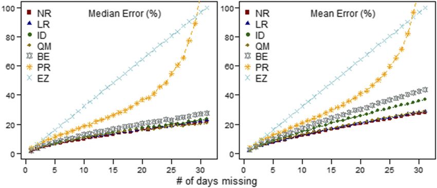
1266               JOURNAL OF APPLIED METEOROLOGY AND CLIMATOLOGY                                              VOLUME 59

Method 6 (PR) is self-contained infilling using only in-       with a given target station are not considered as poten-
formation from the target station to fill missing data.        tial predictor stations for that target station.
Method 7 (EZ) replaces missing values with zeros, po-
                                                                 3) CORRELATION THRESHOLD
tentially causing drastic changes to the distribution.
                                                                 For the NR, LR, QM, and BE approaches, predictor
c. Optimization method
                                                               stations are typically selected based on the strength of
   Drawing on the 25-yr rainfall dataset described above,      their correlation with a target station. The choice of this
we selected a 2-yr sample (January 2013–December               correlation threshold, however, is arbitrary. In prior
2014), the period with the least number of missing ob-         studies, candidate predictor stations were selected using
servations within the dataset, for out-of-sample testing       minimum Pearson correlation coefficient r thresholds of
of the methods. For a given target station, we removed         0.35 (for several gap-filling methods; Eischeid et al.
all observations and then filled the entire time series        2000), 0.5 (for the nearest-neighbor method; Vicente-
using each of the gap-filling approaches and under dif-        Serrano et al. 2009), and 0.88 (for the NR method;

                                                                                                                             Downloaded from http://journals.ametsoc.org/jamc/article-pdf/59/7/1261/4986690/jamcd200007.pdf by guest on 03 August 2020
ferent optimization scenarios. The observed time series        Giambelluca et al. 2013). In this study, the threshold
was then used to cross validate the results.                   correlation between target and predictor stations was
                                                               tested by comparing the errors associated with using
  1) NUMBER OF PREDICTOR STATIONS FOR NR
                                                               predictor stations within six correlation ranges (0.3–0.4,
     AND ID METHODS
                                                               0.4–0.5, 0.5–0.6, 0.6–0.7, 0.7–0.8, and .0.8). First, all
  For both the NR and ID methods, multiple predictor           target stations that were significantly correlated with at
stations can be used to derive an estimate at a target         least one predictor station within each threshold range
station. The number of predictor stations to use must be       are identified (i.e., a station must have a complete range
decided, often in arbitrary fashion. For the NR method,        of correlations with other stations). This allowed for an
Eischeid et al. (2000) suggested using no more than four       equal sample size within each threshold range. The four
predictor stations and that the use of more than four          gap-filling approaches that use correlation as a criterion
predictor stations can degrade the estimates. For the          for selecting a predictor station were applied, and the
ID method, many researchers have suggested the use of          errors produced at each threshold range were analyzed.
three or four predictor stations (e.g., Teegavarapu and        For this analysis the ID method is executed without any
Chandramouli 2005). In this study, we test how the use of      modifications. Correlation thresholds (as opposed to
between 1 and 10 predictor stations can influence the re-      correlation ranges) were also tested using the entire
sults at a target station for both the NR and ID methods.      sample dataset where gap filling was done, and errors
                                                               were calculated using all available predictor stations
  2) ESTABLISHING STATISTICAL RELATIONSHIPS
                                                               below four thresholds (#0.4, ,0.5, ,0.6, and ,0.7).
       BETWEEN STATIONS
                                                                 4) NEIGHBORHOOD OF INFLUENCE
   The NR, LR, QM, and BE methods require that sta-
tistical relationships be established between stations.          The arbitrariness in the choice of the neighborhood
Both Eischeid et al. (2000) and Tardivo (2015) suggest         from which predictor stations are selected has been
that a stable estimation statistic can be derived from 10      identified as a distinct limitation to the ID method
years of overlapping data between stations. Because of         (Teegavarapu and Chandramouli 2005). In this study,
missing data and relatively short periods of record, even      the relationship between distance to the nearest pre-
using a dataset that spans 25 years, requiring a 10-year       dictor station and error (difference between predicted
period of overlap in this present study would eliminate        and observed rainfall) is assessed for all methods. The
most of the available sample stations. Therefore, sta-         distance between each target station and all of the pre-
tistical relationships were established between stations       dictor stations was calculated, and six distance ranges
when at least 1000 days of overlapping data between            (90–117, 65–90, 41–65, 21–41, 4–21, and ,4 km) were
stations were available (note that this was choice and not     selected such that an equal sample size was achieved
an optimized parameter). Statistical relationships be-         within each range. Errors were calculated for gap filling
tween stations were calculated using only data available       done at select target stations using unique predictor
during the 23-year period (1990–2012) so as to avoid use       stations within each range.
of data during the 2013–14 test period. As a subsequent
                                                                 5) WEIGHTING PARAMETERS FOR THE ID
step, the statistical significance of each station relation-
                                                                    METHOD
ship was tested using the correlation between two sta-
tions and all stations relationships that do not have            The arbitrary choice of a weighting parameter l assigned
statistically significant (p # 0.05) positive correlation      to stations when using the ID method is another limitation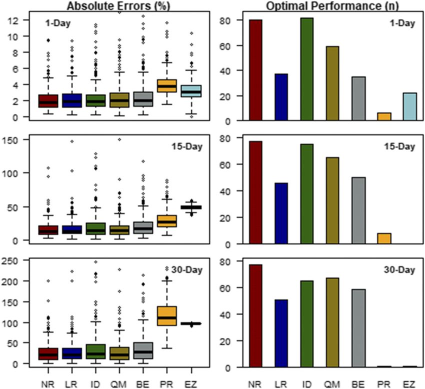
JULY 2020                                        LONGMAN ET AL.                                                     1267

to this method (Teegavarapu and Chandramouli 2005).            (NR, LR, ID, QM, BE, PR, and EZ). The filled daily
With the ID method, the exponent l is typically set to 2       data were then aggregated to monthly totals and com-
(e.g., Shepard 1964; Webster and Oliver 2001). Here we         pared with the observed monthly data. This process is
test how the use of different values of the exponent (l 5      repeated 31 times for each data-gap scenario (between 1
1, 1.5, and 2) influences the results.                         and 31 days missing). For example, to test the effect of
                                                               filling a 10-day gap in a given month, 31 different sam-
  6) RATIO THRESHOLD FOR THE NR METHOD
                                                               ples were created, each with 10 daily values randomly
  Normal ratios are calculated as the long-term mean           removed, and then filled using each method. Errors
of a target station divided by the long-term mean of a         (departures from the actual observed values) are then
predictor station with means based only on overlapping         calculated for each of the filled values and the average of
data periods between stations. Following Longman et al.        both the collective mean and median deviations be-
(2018), a ratio range from 0.3 to 2.7 is used to identify      tween the gap filled and observed monthly rainfall are
candidate predictor stations.                                  calculated. Note that for the PR approach gaps are filled

                                                                                                                             Downloaded from http://journals.ametsoc.org/jamc/article-pdf/59/7/1261/4986690/jamcd200007.pdf by guest on 03 August 2020
                                                               for up to 30 days because at least one observation is
  7) RAIN/NO-RAIN BIAS CORRECTION
                                                               needed for executing this method. Results are only
  One limitation that applies to all of the gap-filling        compared in instances where all of the gap-filling methods
approaches is that they typically do not represent             can be employed. While this reduces the total number
rain/no-rain percentages accurately. For gap-filling methods   of samples, it allows for a homogeneous sample com-
using multiple predictor stations, the number of rain          parison between methods. For each gap size, error
days is generally overpredicted. With multiple predictor       metrics are derived based on a combined sample of
stations, if any of them has nonzero rainfall on a given       308 481 combinations.
day, then the estimated rainfall at the target station will
                                                               e. The added value of gap filling daily data
be nonzero, leading to a bias in the rain day frequency
(Hasan and Croke 2013). In addition, the possibility              Serially complete data are important for a number of
of overestimation of rainfall using the LR and QM              applications including the spatial interpolation of point
methods that use a single predictor station is also present    data to a gridded surface. It can be assumed that the
as rainfall is predicted based on a statistical relationship   denser the station coverage the better the gridded sur-
that could produce daily rainfall . 0 at a target station      face will be. But does this assumption hold for partially
when zero rainfall is observed at a predictor station.         gap-filled data? Here, this assumption was tested using
Over estimation as a result of gap filling creates the need    sample months from the monthly dataset. First, the
for a rain/no-rain correction to be included in the rainfall   complete daily station records of fourteen 31-day months
prediction. Corrections to rainfall estimates, based on        were aggregated to monthly totals. Next, two additional
rain/no-rain characteristics at the closest station (based     monthly datasets were created after 20% of the daily
on Euclidean distance) or the highest correlated station       station records were randomly removed from the time
have been shown to be effective (Teegavarapu et al.            series and another in which the removed stations were
2018). In this work we tested rain/no-rain corrections         gap filled first and then aggregated to monthly. Then,
that were based on both distance and correlation for all       gridded surfaces were created using a climatologically
of the methods and compare the results with gap filling        aided ordinary kriging approach (see Frazier et al. 2016),
in the absence of the rain/no-rain correction.                 using three different monthly rainfall datasets: the
                                                               monthly observed dataset, the monthly dataset with
d. Gap filling at various temporal resolutions
                                                               20% of the stations removed, and the monthly dataset
  Once the optimal parameterization was established            with 20% of the stations filled. Last, the gridded sur-
for each method, the same 2-year daily time series             faces created with those three datasets are compared.
(2013–14) was gap filled and the methods were assessed
                                                               f. Performance criteria metrics and statistical tests
on their ability to predict rainfall at each target station
during this long artificial gap. The 2-year reconstructed        Several statistics are used to measure the effectiveness
time series was tested against the observed time series        of the gap-filling approaches. The mean bias error
and errors assessed. Errors associated with gap filling        (MBE) is used as measure of the mean over/under pre-
small gaps in station record (between 1 and 31 days) are       diction of a method. The mean absolute error (MAE) is
also tested using the following steps. For all complete        used as measure to see how close simulated values are to
31-day station/months in the sample dataset (n 5 321), a       observed values assuming the data are normally distrib-
random day is removed from each monthly time series            uted. The root-mean-square error (RMSE) is used to
and the gap is filled using each of the seven methods          measure the overall spread of the errors in a normal
1268               JOURNAL OF APPLIED METEOROLOGY AND CLIMATOLOGY                                                VOLUME 59

distribution. The median absolute error (MED) is used            1) NUMBER OF PREDICTOR STATIONS
as a measure of central tendency in a nonnormal dis-
                                                                  For both the NR and the ID methods, ANOVA re-
tribution. The coefficient of determination R2 is used to
                                                               sults showed no significant advantage to using more than
measure the linear correlation between observed and
                                                               one predictor station to gap fill rainfall at a target sta-
filled data. These metrics among others are widely used
                                                               tion. The optimal number of predictor stations to use
for the performance of comparison of gap-filling methods
                                                               varied by metric. However, for the NR method the
(Kim and Ryu 2016).
                                                               lowest MAE and RMSE were obtained when three
   Comparative analysis of the errors associated with
                                                               stations were used and for the ID method when 10 stations
both the optimization and execution of the individual
                                                               were used. Subsequent iterations using these methods
gap-filling methods are carried out using both para-
                                                               were parameterized accordingly.
metric and nonparametric statistical tests depending on
the shape of the distribution. In instances where error          2) CORRELATION THRESHOLD
distributions are normal and variances are equal, a one-

                                                                                                                               Downloaded from http://journals.ametsoc.org/jamc/article-pdf/59/7/1261/4986690/jamcd200007.pdf by guest on 03 August 2020
way analysis of variance (ANOVA) was used to deter-               Thirteen target stations with at least one predictor
mine the degree to which mean errors differ between the        station in each of the six correlation threshold ranges
gap-filling methods. When significant differences were         were identified. Results show no differences in the MED
identified, the Tukey’s honestly significant difference        error between the NR, ID, and QM methods for pre-
(HSD) test was used to test for significant differences in     dictor stations above the r 5 0.5–0.6 range (Figs. 2a,b).
each of the pairwise comparisons. For nonnormally              Below this range, the ID method (which was executed
distributed data, the Wilcoxon rank-sum test was used          without any modifications) produces significantly lower
to identify significant differences in median errors. For      MED errors than all of the other methods. MAE errors
both parametric and nonparametric tests, the null hy-          are significantly lower for the ID method below the r 5
pothesis H0 is that differences between observed and           0.6–0.7 range. Error was also assessed using MAE and
estimated rainfall are from the same continuous distri-        MED for sets of all available stations at four correlation
bution for any two gap-filled datasets. The alternative        thresholds (r , 0.4, ,0.5, ,0.6, and ,0.7). Results show
hypothesis Ha is that these two datasets are from dif-         that, when compared with the other methods, the ID
ferent continuous distributions. The hypothesis tests          method produces significantly lower MED errors for
were carried out at a statistical significance level of 5%     predictor stations below the r 5 0.5 threshold and sig-
(a 5 0.05).                                                    nificantly lower MAE errors for stations below the r 5
                                                               0.6 threshold (Fig. 3). For subsequent portions of this
g. Probability of precipitation                                analysis and for methods requiring the selection of
  Daily probability of precipitation (PoP) can be used to      predictor stations based on correlation, the r 5 0.6
quantify the frequency of spurious nonzero rainfall in-        threshold is used to identify candidate predictor sta-
troduced during the gap-filling process (e.g., Newman          tions for the four gap-filling methods that use the cor-
et al. 2015). The differences in climatological mean PoP       relation as a criterion for selecting candidate predictor
as a result of gap filling are evaluated for all of the var-   stations.
ious gap sizes. First, the PoP at each station is calculated
                                                                 3) NEIGHBORHOOD OF INFLUENCE
as the number of observed rain days [days with .
0.15 mm of rainfall (RF)] divided by the total number of         The ability to fill daily rainfall using predictor stations
days in the time series. PoP is then calculated for the        at six different distance thresholds was tested. On av-
predicted datasets and the difference between the pre-         erage the closest predictor station is 5.5 km away from a
dicted and observed datasets is used as measure of             given target station and the average distance to the next
prediction bias.                                               closest station is 8.9 km with high variance across the
                                                               dataset. In total, 14 target stations having a nonzero
3. Results                                                     sample of predictor stations in each of the six distance
                                                               threshold ranges (roughly 23-km bins) were identified
a. Method optimization
                                                               for this test. Note that for the methods that require es-
  Of the 75 observation stations examined in this study,       tablished statistical relationship with another station,
only 36 met the criteria necessary for the execution of all    the rank correlation was only considered when multiple
of the gap-filling methods. On average, station records in     predictor stations were available at a given distance
the 2-year sample were 93% complete (range 59%–                threshold. Results show no statistical differences in the
100%); therefore, error statistics are based on a sample       MAE or MED between methods at any of the distance
of approximately 24 000 station-days.                          thresholds analyzed (Figs. 2c,d). In general, both the
JULY 2020 LONGMAN ET AL. 1269
Downloaded from http://journals.ametsoc.org/jamc/article-pdf/59/7/1261/4986690/jamcd200007.pdf by guest on 03 August 2020
FIG. 2. (left) MAE and (right) MED associated with gap filling daily rainfall using predictor
stations (a),(b) within six unique correlation ranges (n 5 13 stations) and (c),(d) at six unique
distance ranges (n 5 14); the vertical dashed line in (a) and (b) marks the threshold at which the
error produced when using the ID method is significantly lower than the error produced using
all of the other approaches.
MAE and MED errors were higher at further distances while the DIST correction produced the least bias for
from a target station. the ID method. For all of the methods, the range of
errors was the smallest when using the COR correction.
4) WEIGHTING PARAMETERS FOR THE ID
In subsequent portions of this analysis, the COR bias
METHOD
correction was applied to the NR, LR, and QM methods,
The ID approach was tested using three different and the DIST correction was applied to the ID method.
weighting approaches (l 5 1, 1.5, and 2). No statistical
b. Evaluation of methods
differences were identified between the distributions
of errors for the different approaches. The lowest er-
1) OPTIMAL METHOD COMPARISON (LONG GAPS)
rors were obtained when the standard exponent of two
(l 5 2) was utilized. Therefore, the weight of l 5 2 was Five gap-filling approaches were assessed on their
used in the execution of the ID method in subsequent ability to accurately fill a large (;2 year) gap in a time
analyses. series. This ‘‘long’’ 2-year gap allows for metrics to be
calculated representing some seasonal and interannual
5) RAIN/NO-RAIN BIAS CORRECTION
RF variability in Hawaii. On average, 663 6 79 days of
The bias correction methods were evaluated based on data were filled at each of the 36 stations available for
the difference between observed and estimated PoP comparison. Results were fairly similar among methods
calculated after removing 20% of the data and gap fill- over this long gap (Fig. 5). Comparative statistics for all
ing. Figure 4, shows the deviation in PoP for predictions performance metrics are presented in Table 1. No sta-
made with the five gap-filling methods with the distance tistical difference was identified in the error distribu-
(DIST) and correlation (COR) bias corrections and tions between any of the five gap-filling methods for any
without a bias correction (NO). For the NR, LR, ID, and of the eight performance metrics considered. The lowest
QM gap-filling approaches, results show that the inclu- normalized MAE (62.2%) was obtained using the LR
sion of either a distance or correlation based bias cor- method, and the lowest MED (12.5% 6 8.8%) was ob-
rection significantly reduces the inclusion of spurious tained using the NR method. The highest R2 (62%) was
rainfall during gap filling. The distribution means, de- obtained using the ID method. MED errors ranged from
rived from Fig. 4, were closest to zero when the COR 12.5% to 16.5% across the methods suggesting that all
method was used for the NR, LR, and QM methods, methods do a fairly reasonable job of gap filling longer1270 JOURNAL OF APPLIED METEOROLOGY AND CLIMATOLOGY VOLUME 59
Downloaded from http://journals.ametsoc.org/jamc/article-pdf/59/7/1261/4986690/jamcd200007.pdf by guest on 03 August 2020
FIG. 3. (left) MAE and (right) MED for five gap-filling approaches including NR, LR, ID, QM,
and BE and under four correlation thresholds: (a), (b) #0.4, (c), (d) # 0.5, (e), (f) # 0.6, and
(g), (h) # 0.7. The red star indicates where the errors produced from the ID method are signif-
icantly lower than the errors produced from all of the other methods; data points exceeding the
maximum error [75th percentile (top of box) + 1.5 3 the interquartile range (whisker)] are plotted
as outliers of the data, and those outliers exceeding the y-axis bounds on the graph are not shown.
records. In general, the MAE was high (62.2%–71.9%) determined to be nonnormal; therefore, nonparametric
for all methods, which suggests that large outliers are tests were used to identify statistical differences between
present in all of the gap-filled datasets. This is especially the distributions and for each of the 31 different gap
true for the BE method, which had the highest MAE sizes. Results indicated no consistent statistical differ-
(71.9%). The difference in PoP errors were generally ences between the NR, LR, ID, and QM methods for
negative but small for all of the methods. This suggests any gap size tested. No significant differences were
that while the rain/no-rain correction does well at re- found between the ID and BE methods, and all methods
ducing of spurious rainfall created during the filling were significantly better than the PR and EZ methods.
process it also produces artificial zero values in in- Figure 7 shows the distribution of errors for 1-, 15-, and
stances where a positive rainfall value should have 30-day gaps and the frequency for which a single method
been predicted. outperformed the other methods as based on minimum
deviation between observed and gap-filled monthly
2) DATA AGGREGATION ERROR (SHORT GAPS)
rainfall totals (Table 2). For 1-day gaps, mean errors
Daily data were gap filled at each station and for each ranged from 2.1% to 4.0%, and the NR method pro-
sample month using the same five gap-filling methods duces both the lowest mean (2.1%) and median (1.8%)
that were previously analyzed as well as the PR and errors. For 15-day gaps, mean errors ranged from
EZ methods described earlier. In total, 231 complete 16.6% to 48.3% and, again, the NR method had the
station-months were used. First daily data were aggre- lowest mean (16.6%) and median (13.1%) errors. For
gated to a monthly time step and then the difference 30-day gaps, the NR method had the lowest mean error
between observed and gap-filled data were compared. (27.4%), but the QM method had the lowest median
Median and mean deviations between observed and error (20.3%). In general, the NR method most con-
gap-filled monthly rainfall totals for 1–31-day data gaps sistently performed as the optimal method for all gap
are presented in Fig. 6. The distribution in errors was sizes considered.JULY 2020 LONGMAN ET AL. 1271
filled data is shown in Fig. 8. Note that in Fig. 8a com-
posite errors are a result of missing data and in Fig. 8b
errors are a result of the gap filling. Errors were found in
both composites, but the mean and median errors were
higher in the composite with the missing station data. In
general, in the missing data composite, there was a large
overprediction on the windward side of the island, which
was greatly reduced in the gap-filled composite. The
individual grid cells produced with and without gap
filling were also compared directly with observations
(Figs. 9a,b). For the gap-filled product, the correlation
between observed and predicted rainfall was higher and
all errors were considerably lower for the product cre-
Downloaded from http://journals.ametsoc.org/jamc/article-pdf/59/7/1261/4986690/jamcd200007.pdf by guest on 03 August 2020
ated with missing observations. The distribution of er-
rors was much smaller in the composite with filled data
(Fig. 9d) when compared to the distribution with missing
data (Fig. 9c) and the range of both mean (Fig. 9e) and
median errors was smaller for the gap-filled product as
can been in seen in comparison side-by-side compari-
sons in Fig. 9e and Fig. 9f, respectively. This comparison
demonstrates the added value of gap filling monthly
rainfall prior to spatial interpolation of point data. We
do acknowledge that the location and magnitude of the
FIG. 4. Differences in the PoP between observed data and gap-
error would undoubtedly vary depending on which sta-
filled data under three bias correction approaches— NO, COR, tions are removed/filled prior to the interpolation and
and DIST (middle column)—for five gap-filling methods: NR, LR, that, despite gap filling, errors are still present in the
ID, QM, and BE. Data points falling outside the Q1–Q3 range are composite.
plotted as outliers of the data.
4. Summary and future work
Surprisingly, the EZ method was the optimal method
22 times for 1-day data gaps and produced significantly The primary objectives of this study were to deter-
lower errors than using the PR method. This is explained mine the performance of gap filling daily rainfall in
by the fact that the EZ method does not introduce any Hawaii for data gaps of various size and to identify the
additional rainfall; therefore, setting 1-day gaps to zero value of gap filling daily rainfall prior to the spatial in-
in dry months is often an accurate estimate. For gaps terpolation of monthly values. First, five gap-filling
from 3 to 26 days, however, the PR method was a sig- methods were optimized and then tested on a large
nificantly better choice than the EZ method. Errors for (2 yr) data gap. Then, these same five methods and two
both of these methods were significantly higher, and, additional methods were tested to determine the error
therefore, they should not be employed regardless of the associated with filling submonthly gaps (between 1 and
gap size. 31 days missing) by calculating the error associated
with aggregating gap-filled daily rainfall to monthly
3) ADDED VALUE OF GAP FILLING
accumulations.
The added value of gap filling daily rainfall prior The optimization analysis highlighted the importance
to the spatial interpolation of monthly rainfall was of tailoring a gap-filling approach to a specific area
assessed by creating a gridded surface with and with- of interest, as the density of a station network, topo-
out gap filling and then comparing these products to a graphical setting, and area of influence will be unique for
gridded surface created with complete observations. each study site. Optimization of the selected gap-filling
Missing daily rainfall was gap filled using first the NR approach is a critical step that should not be overlooked.
method when statistical thresholds were met and the Results in this study suggest that both the correlation
ID method for all other instances. The combined use and distance between a target and predictor station
of these methods allows for the creation of the serially are important factors in producing a quality estimate.
complete datasets A 14-month composite of the dif- As expected, larger distance or lower correlations
ferences between gridded surfaces with missing and correspond to larger errors. More importantly, the1272 JOURNAL OF APPLIED METEOROLOGY AND CLIMATOLOGY VOLUME 59
Downloaded from http://journals.ametsoc.org/jamc/article-pdf/59/7/1261/4986690/jamcd200007.pdf by guest on 03 August 2020
FIG. 5. Gap-filling errors across eight unique metrics—(a) MBE, (b) RMSE, (c) MAE,
(d) relative MAE, (e) median absolute error (MED AE), (f) relative MED (MED AE), (g) R2,
and (h) the difference in the PoP and gap-filled datasets—for five gap-filling methods: NR, LR,
ID, QM, and BE. Data points falling outside the Q1–Q3 range are plotted as outliers of the
data, and those outliers exceeding the y-axis bounds on the graph are not shown.
establishment of a correlation threshold allows for a used in place of another method. This of course is also
decision to be made as to when to choose between dif- dependent on the availability of stations used to properly
ferent methods. To achieve serially complete data using execute the ID method. In some instances, where a net-
the methods described in this study, the ID method must work may be less dense than the one utilized in this study,
be used exclusively or in combination with another it might be better to select a station with a low correlation
method due to the fact that the other methods have as opposed to a station at greater distance or to use a
minimum statistical requirements that may not be met all completely different gap-filling method to address the
of the time. To this end, identifying a correlation thresh- issue. Because of the density of the stations used in this
old is a way to determine when the ID method should be analysis, the area of influence was not a limiting factor.
TABLE 1. Average errors associated with filling a large (;2 yr) gap in the records at 36 rainfall stations. REL MAE is the average
relative absolute mean error, REL MED is the average relative absolute median error, D-PoP is the average difference in the probability
of rainfall between the observed and the gap-filled data at 36 sample stations, and the other metrics are defined in section 2f. The lowest
errors for each metric are shown in boldface font. The methods are defined in section 1 and described in section 2b.
REL REL
MBE (mm) MAE (mm) MAE (%) RMSE (mm) MED (mm) MED (%) R2 D-PoP (%)
Std Std Std Std Std Std Std Std
Method Mean dev Mean dev Mean dev Mean dev Mean dev Mean dev Mean dev Mean dev
NR 20.31 60.7 3.2 62.1 63.4 624.3 7.8 64.4 0.9 61.0 12.5 68.8 0.61 60.25 20.5 68.7
LR 20.19 61.0 3.3 62.1 62.2 620.0 7.8 64.0 1.2 61.2 16.5 612.8 0.61 60.21 21.7 610.3
ID 20.15 62.3 3.3 62.1 65.4 623.7 8.0 64.3 1.0 61.0 14.5 610.9 0.62 60.22 21.4 616.0
QM 0.21 61.1 3.4 62.3 66.3 624.3 8.5 64.7 1.0 61.1 13.2 610.1 0.61 60.20 22.8 68.9
BE 20.34 62.3 3.6 62.3 71.9 634.4 8.6 64.6 1.0 61.0 14.1 610.7 0.60 60.21 21.3 610.3JULY 2020 LONGMAN ET AL. 1273
Downloaded from http://journals.ametsoc.org/jamc/article-pdf/59/7/1261/4986690/jamcd200007.pdf by guest on 03 August 2020
FIG. 6. (left) MED and (right) MAE between observed monthly total rainfall and monthly rainfall, when daily gaps are
filled, for between 1 and 31 days missing and for seven gap-filling methods: NR, LR, ID, QM, BE, PR, and EZ.
Another essential optimization approach is the in- of this correction also resulted in a small negative bias in
clusion of a rain/no-rain bias correction. For all of the the overall estimates.
methods tested, using either the COR or DIST cor- For longer (2 yr) gaps, all five of the gap-filling ap-
rection significantly reduced instances where spurious proaches produced similar results, and no statistical dif-
rainfall was added to the gap-filled dataset. The inclusion ferences were identified between the error distributions.
FIG. 7. (left) Absolute errors between observed monthly rainfall sums and monthly sums with daily
gaps filled and (right) the frequency in which a given method was optimal for a given month for (top)
1 day of missing data, (middle) 15 days of missing data, and (bottom) 30 days of missing data for seven
infilling methods: NR, LR, ID, QM, BE, PR, and EZ. Boxplot data falling outside the Q1–Q3 range are
plotted as outliers of the data, and those outliers exceeding the y-axis bounds on the graph are not shown.1274 JOURNAL OF APPLIED METEOROLOGY AND CLIMATOLOGY VOLUME 59
TABLE 2. Absolute mean and median (MED) deviations between gap-filled and observed monthly rainfall for seven infilling methods
and for three missing data scenarios, along with RMSE. All metrics are percentages. The lowest errors for each metric are shown in
boldface font.
1-day gap 15-day gap 30-day gap
MED Mean RMSE MED Mean RMSE MED Mean RMSE
NR 2.2 2.8 1.7 17.1 23.3 4.8 25.0 37.5 6.1
LR 2.3 2.8 1.7 18.5 24.7 5.0 28.9 41.7 6.5
ID 2.4 3.6 1.9 20.1 33.9 5.8 29.2 59.2 7.7
QM 2.3 3.3 1.8 18.7 30.4 5.5 27.0 51.0 7.1
BE 2.5 3.7 1.9 21.1 37.7 6.1 31.5 65.7 8.1
PR 4.1 4.3 2.1 30.5 34.0 5.8 121.9 130.4 11.4
EZ 3.1 3.2 1.8 48.6 48.6 7.0 96.9 96.8 9.8
Downloaded from http://journals.ametsoc.org/jamc/article-pdf/59/7/1261/4986690/jamcd200007.pdf by guest on 03 August 2020
For smaller gaps, no statistical differences were found One of the most important findings of this study is the
between these same five methods. However, all of these added value that gap filling a daily rainfall time series
methods produced errors significantly lower than the PR has prior to spatial interpolation of these data. In diverse
and EZ methods. These results show that under no cir- topographical areas such as Hawaii Island, gap filling
cumstances should either of these methods be employed critical stations can help to capture complex rainfall
(regardless of the gap size). For our analysis of smaller gradients that exist there.
gaps, the QM method produced the lowest median error The method described in this paper can be readily
when gaps were greater than 15 days. However, mean adapted for use with other datasets at a daily temporal
errors were consistently lowest when using the NR resolution. The most appropriate gap-filling approach
method. Given that the NR approach utilizes multiple for any unique station may vary in both space and
predictor stations, this has a smoothing effect on the time, especially considering that all the methods
estimates and can reduce errors associated with large presented here are dependent on information from
outliers. Overall, the NR method was the most consis- predictor stations that may or may not be available
tent at reproducing monthly rainfall and was consis- on a given day. Also, because many of these methods
tently the most optimal method overall. The results in require established statistical relationships between
this study were similar to those of Tardivo and Berti target and predictor stations, their ability to fill all
(2013), who also found that the NR method (using up to gaps within a dataset may be limited. Thus, filling a
three predictor stations) was optimal among several dataset to completion may require the use of multiple
other methods for gap filling daily rainfall in Italy. approaches.
FIG. 8. Fourteen-month composite of deviations between a gridded surface created with monthly observations
and a gridded surface created with (a) 20% of the stations removed and (b) 20% of the stations filled, and their
associated MBE and MED.JULY 2020 LONGMAN ET AL. 1275
Downloaded from http://journals.ametsoc.org/jamc/article-pdf/59/7/1261/4986690/jamcd200007.pdf by guest on 03 August 2020
FIG. 9. Fourteen-month composite of gridded estimates of observed rainfall (x axis) compared
with gridded estimates made with (a) 20% of the observations missing (RF data are in milli-
meters) and (b) 20% of the observations filled; frequency distributions of normalized absolute
rainfall for gridded estimates made with (c) 20% of the observations missing and (d) 20% of the
observations filled; (e) mean and (f) median deviations in rainfall between gridded estimates
made with observed rainfall data, and gridded estimates made with 20% of the data missing and
20% of the data filled. In (e) and (f), data falling outside the Q1–Q3 range are plotted as outliers of
the data, and those outliers exceeding the y-axis bounds on the graph are not shown.
The results of this study will be used to support an Climate Adaptation Science Center for continued sup-
ongoing research effort to produce a serially complete port. The National Center for Atmospheric Research
daily rainfall dataset for the State of Hawaii (from 1990 is a major facility sponsored by the National Science
to present day), which is part of a bigger project to Foundation under Cooperative Agreement 1852977.
develop a near-real-time data acquisition and rainfall
mapping system for the State of Hawaii. REFERENCES
Acknowledgments. We thank Abby Frazier, East- Adhikary, S. K., N. Muttil, and A. G. Yilmaz, 2016: Genetic
programming-based ordinary kriging for spatial interpolation
West Center, and Mike Nullet, Department of Geography of rainfall. J. Hydrol. Eng., 21, 04015062, https://doi.org/
and Environment, University of Hawaiʻi at M anoa. 10.1061/(asce)he.1943-5584.0001300.
Funding for the Hawaii EPSCoR Program, which sup- Caldera, H. P. G. M., V. R. P. C. Piyathisse, and K. D. W. Nandalal,
ported this work, is provided by the National Science 2016: A comparison of methods of estimating missing daily
Foundation’s Research Infrastructure Improvement (RII) rainfall data. Eng. J. Inst. Eng. Sri Lanka, 49, 1–8, https://
doi.org/10.4038/engineer.v49i4.7232.
Track-1: ‘Ike Wai: Securing Hawaii’s Water Future Award
Eischeid, J. K., C. B. Baker, T. R. Karl, and H. F. Diax, 1995: The
OIA-1557349. Andrew Newman was funded by the U.S. quality control of long-term climatological data using objective
Army Corps of Engineers Climate Preparedness and data analysis. J. Appl. Meteor., 34, 2787–2795, https://doi.org/
Resilience Program. We also thank the Pacific Island 10.1175/1520-0450(1995)034,2787:TQCOLT.2.0.CO;2.You can also read