Classifying Goliath Grouper (Epinephelus itajara) Behaviors from a Novel, Multi-Sensor Tag

Page created by Greg Casey
 
CONTINUE READING
Classifying Goliath Grouper (Epinephelus itajara) Behaviors from a Novel, Multi-Sensor Tag
sensors
Article
Classifying Goliath Grouper (Epinephelus itajara) Behaviors
from a Novel, Multi-Sensor Tag
Lauran R. Brewster 1, * , Ali K. Ibrahim 1,2 , Breanna C. DeGroot 1 , Thomas J. Ostendorf 1 , Hanqi Zhuang 2 ,
Laurent M. Chérubin 1 and Matthew J. Ajemian 1

                                          1   Harbor Branch Oceanographic Institute, Florida Atlantic University, Fort Pierce, FL 34946, USA;
                                              aibrahim2014@fau.edu (A.K.I.); bdegroot2017@fau.edu (B.C.D.); tostendorf@fau.edu (T.J.O.);
                                              lcherubin@fau.edu (L.M.C.); majemian@fau.edu (M.J.A.)
                                          2   Department of Electrical Engineering and Computer Science, Florida Atlantic University,
                                              Boca Raton, FL 33431, USA; zhuang@fau.edu
                                          *   Correspondence: lbrewster@fau.edu; Tel.: +1-772-242-2638

                                          Abstract: Inertial measurement unit sensors (IMU; i.e., accelerometer, gyroscope and magnetometer
                                          combinations) are frequently fitted to animals to better understand their activity patterns and energy
                                          expenditure. Capable of recording hundreds of data points a second, these sensors can quickly
                                          produce large datasets that require methods to automate behavioral classification. Here, we describe
                                          behaviors derived from a custom-built multi-sensor bio-logging tag attached to Atlantic Goliath
                                          grouper (Epinephelus itajara) within a simulated ecosystem. We then compared the performance of
                                          two commonly applied machine learning approaches (random forest and support vector machine) to
                                          a deep learning approach (convolutional neural network, or CNN) for classifying IMU data from
         
                                   this tag. CNNs are frequently used to recognize activities from IMU data obtained from humans
Citation: Brewster, L.R.; Ibrahim,
                                          but are less commonly considered for other animals. Thirteen behavioral classes were identified
A.K.; DeGroot, B.C.; Ostendorf, T.J.;     during ethogram development, nine of which were classified. For the conventional machine learning
Zhuang, H.; Chérubin, L.M.; Ajemian,      approaches, 187 summary statistics were extracted from the data, including time and frequency
M.J. Classifying Goliath Grouper          domain features. The CNN was fed absolute values obtained from fast Fourier transformations of the
(Epinephelus itajara) Behaviors from a    raw tri-axial accelerometer, gyroscope and magnetometer channels, with a frequency resolution of
Novel, Multi-Sensor Tag. Sensors          512 data points. Five metrics were used to assess classifier performance; the deep learning approach
2021, 21, 6392. https://doi.org/          performed better across all metrics (Sensitivity = 0.962; Specificity = 0.996; F1 -score = 0.962; Matthew’s
10.3390/s21196392                         Correlation Coefficient = 0.959; Cohen’s Kappa = 0.833) than both conventional machine learning
                                          approaches. Generally, the random forest performed better than the support vector machine. In
Academic Editor: Stefano Mariani
                                          some instances, a conventional learning approach yielded a higher performance metric for particular
                                          classes (e.g., the random forest had a F1 -score of 0.971 for backward swimming compared to 0.955 for
Received: 23 August 2021
Accepted: 19 September 2021
                                          the CNN). Deep learning approaches could potentially improve behavioral classification from IMU
Published: 24 September 2021              data, beyond that obtained from conventional machine learning methods.

Publisher’s Note: MDPI stays neutral
                                          Keywords: accelerometer; magnetometer; gyroscope; classification; random forest; support vector
with regard to jurisdictional claims in   machine; deep-learning; bio-logging
published maps and institutional affil-
iations.

                                          1. Introduction
                                               The past few decades have seen the development, miniaturization and cost reduc-
Copyright: © 2021 by the authors.         tion of a variety of sensors that can be attached to animals to monitor their behavior,
Licensee MDPI, Basel, Switzerland.        physiology and environment [1]. Data (archival) loggers are particularly appealing if the
This article is an open access article    device can be retrieved due to their capacity to store large datasets, allowing for high
distributed under the terms and           sampling frequencies and thus fine-scale monitoring [2]. Often, sensors are used in tandem
conditions of the Creative Commons        to better identify and contextualize behavior. For example, a tri-axial accelerometer can
Attribution (CC BY) license (https://     be used to measure body motion and posture in the three orthogonal planes, through
creativecommons.org/licenses/by/          dynamic and gravitational forces, respectively. In turn, distinct behaviors corresponding
4.0/).

Sensors 2021, 21, 6392. https://doi.org/10.3390/s21196392                                                     https://www.mdpi.com/journal/sensors
Classifying Goliath Grouper (Epinephelus itajara) Behaviors from a Novel, Multi-Sensor Tag
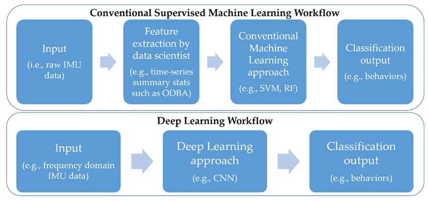
Sensors 2021, 21, 6392                                                                                            2 of 20

                         to these waveform signatures can be identified (through direct-observation, i.e., “ground-
                         truthing”) or inferred, which has made them a popular choice for scientists aiming to
                         understand the activity of an animal in the wild. When used in conjunction with sensors
                         that provide information on the body’s angular velocity and rotation—through a gyroscope
                         and magnetometer, respectively—the ability to reconstruct and differentiate behaviors
                         can be improved [3–5]. However, with each sensor potentially yielding millions of data
                         points, manually deciphering behaviors from these inertial measurement unit (IMU) data
                         sets is impractical. As such, numerous machine learning (ML) methods have been em-
                         ployed to automate the process of classifying animal-borne sensor output into behavioral
                         classes [6–9].
                               Murphy [10] defines ML as “a set of methods that can automatically detect patterns
                         in data, and then use the uncovered patterns to predict future data, or to perform other
                         kinds of decision making under uncertainty”. ML is typically divided into two main types,
                         supervised and unsupervised learning, each with advantages and disadvantages [8]. In su-
                         pervised learning, a training data set is required whereby the input vector(s) x (e.g., sensor
                         channel features) and associated outcome measure/label in vector y (e.g., behavior) are
                         known. Once the input vectors can be appropriately mapped to the outcome, the algorithm
                         can be used to make predictions from new input data [11]. This is termed supervised learn-
                         ing, as the outcome label is provided by an “instructor” who tells the ML algorithm what
                         to do. If an animal cannot be housed in captivity for direct observation, or simultaneously
                         fitted with the sensor(s) and a video camera while in situ, building a detailed training
                         set may not be possible. In such instances, unsupervised learning can be implemented.
                         Pre-defined classes are not provided by an instructor (hence “unsupervised learning”), but
                         rather the algorithm finds structure in the data, grouping it based on inherent similarities
                         between input variables [11]. While the terms supervised and unsupervised learning help
                         to categorize some of the methods available, the two concepts are not mutually exclusive
                         and can be used in tandem when labeled data is available for only a portion of the dataset
                         (e.g., semi-supervised, multi-instance learning).
                               Recently, deep learning approaches have become popular for modeling high-level
                         data in areas such as image classification [12], text classification [13], medical data classi-
                         fication [14] and acoustic sound classification [15]. Unlike supervised machine learning
                         approaches, deep learning is a form of ML that does not require a manual extraction of
                         features for training the model but instead can be fed raw data (Figure 1). Its development
                         was driven by the challenges faced by conventional ML algorithms including the inability
                         to generalize well to new data, particularly when working with high-dimensional data and
                         the computational power required to do so.
                               Various deep learning approaches have been applied to accelerometer data for human
                         activity classification including convolutional neural networks (CNNs), long short-term
                         memory (LSTM) and a combination of the two [16–24]. Aviléz-Cruz et al. [19] proposed a
                         deep learning model that achieved 100% accuracy across six activities, compared with 98%
                         and 96% for the two most competitive conventional ML approaches (Hidden Markov Model
                         and support vector machine, SVM, respectively). The model had three CNNs working in
                         parallel, all receiving the same input signal from a tri-axial accelerometer and gyroscope.
                         The feature maps of the three CNNs were flattened and concatenated before being passed
                         into a fully connected layer and finally an output layer with a Softmax activation (a function
                         that converts the numbers/logits generated by the last fully connected layer, into a proba-
                         bility that an observation belongs to each potential class [25]). Other studies demonstrate
                         the relevance of using LSTM networks for human activity recognition [17,20–23]. Lastly,
                         a few studies have suggested augmenting CNNs with LSTM layers [26]. For example,
                         Karim et al. [26] proposed a model architecture in which a three-layer CNN and an LSTM
                         layer extract features from sensor data in parallel. The resulting feature vectors are then
                         concatenated and passed into a Softmax classification layer. Although deep learning can
                         yield improved classifier performance over conventional ML methods, it has been sparsely
                         applied for animal behavior detection from IMU data [8].
Classifying Goliath Grouper (Epinephelus itajara) Behaviors from a Novel, Multi-Sensor Tag
Sensors 2021, 21, 6392                                                                                            3 of 20

                               Within the realm of marine fishes, IMU sensors have been widely applied to highly
                         mobile species including sharks [27–29], Atlantic bluefin tuna (Thunnus thynnus) [30],
                         dolphin fish (Coryphaena hippurus) [31] and amberjack (Seriola lalandi) [32], providing insight
                         into biomechanics, activity patterns, energy expenditure, diving and spawning behavior.
                         However, application of IMUs to more sedentary species that persist predominantly over
                         highly complex structures, such as natural and artificial reefs, are rarer. These species, for
                         example grouper, can be expected to engage in different behaviors to that of highly mobile
                         species and present a different activity budget.
                               Groupers (family Epinephelidae) are comprised of more than 160 species of commer-
                         cially and recreationally important fishes that inhabit coastal areas of the tropics and
                         subtropics [33]. This family of long-lived fishes shares life history traits that make them
                         particularly vulnerable to overfishing, including: late sexual maturity, protogyny, and the
                         formation of spawning aggregations [34–37]. The Atlantic Goliath Grouper (Epinephelus
                         itajara Lichtenstein 1822; hereafter referred to as Goliath grouper) is one of the largest
                         grouper species, capable of attaining lengths of 2.5 m and exceeding 400 kg [38]. The
                         species ranges from North Carolina to Brazil and throughout the Gulf of Mexico [39]. Much
                         of our understanding of Goliath grouper behavior has been learned from divers, from
                         underwater video footage, and observing animals in captivity (e.g., feeding kinematics [40],
                         abundance [41]). Passive acoustic monitoring of sound production (e.g., associated with
                         spawning behavior) [42,43] and modest acoustic telemetry work has provided some insight
                         into site fidelity and coarse horizontal and vertical movement [44]. To date, no studies
                         have documented the fine-scale behavior of this species. IMUs provide the opportunity
                         to learn about fine-scale Goliath grouper activity patterns over a range of temporal scales,
                         and the energetic implications. Additionally, IMUs can yield insight into, inter alia, mating
                         behavior, habitat selection and responses to environmental variables [45,46].
                               Accelerometer transmitters have been used to determine activity levels (active ver-
                         sus inactive) [47] and feeding behavior [48] of captive red-spotted groupers (Epinephelus
                         akaara). An accelerometer-gyroscope data logger was used to identify feeding and escape
                         response behavior of captive White-streaked grouper (Epinephelus ongus) [3]. In both stud-
                         ies, behaviors were validated using underwater video cameras situated in the tank. To our
                         knowledge, no studies have used IMU sensors to elucidate the behavior of grouper species
                         at liberty. However, as one of the largest grouper species, Goliath grouper can be equipped
                         with multi-sensor tags that include a video camera for validation of IMU data obtained
                         from individuals in the wild.
                               The goals of this study were to: (a) obtain ground-truthed body movement data
                         from a custom-made tag fitted to Goliath grouper, which could be used to develop a
                         behavioral classifier; (b) develop two conventional ML approaches, using handcrafted
                         features, to classify behavior from the tag data; (c) design a deep learning approach using
                         CNN and frequency representations of IMU data; and (d) compare the performance of the
                         conventional ML approaches to the deep learning approach to determine the preferred
                         method for identifying and studying behaviors from animals at liberty. Knowledge of the
                         fine-scale activity of these animals can help us understand the ecology of this species, a key
                         research need highlighted by the International Union for the Conservation of Nature [39].
Classifying Goliath Grouper (Epinephelus itajara) Behaviors from a Novel, Multi-Sensor Tag
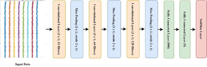
Sensors 2021, 21, 6392                                                                                                                      4 of 20
Sensors 2021, 21, x FOR PEER REVIEW                                                                                                        4 of 21

                                 Figure
                                 Figure 1.
                                         1. Simplified
                                            Simplified schematic
                                                       schematic showing  the workflow
                                                                  showing the workflow of
                                                                                        of conventional
                                                                                           conventionalmachine
                                                                                                        machinelearning
                                                                                                                learningapproaches
                                                                                                                         ap-
                                 proaches   versus deep  learning approaches. IMU = inertial measurement unit, ODBA   = overall
                                 versus deep learning approaches. IMU = inertial measurement unit, ODBA = overall dynamic body  dy-
                                 namic body acceleration, SVM = support vector machine, RF = random forest, CNN = Convolu-
                                 acceleration, SVM = support vector machine, RF = random forest, CNN = Convolutional Neural
                                 tional Neural Network.
                                 Network.

                                 2.
                                 2. Materials
                                    Materials and
                                               and Methods
                                                    Methods
                                 2.1.
                                 2.1. Study
                                      Study Site
                                            Site and
                                                 and Capture
                                                     Capture
                                      Goliath
                                       Goliath groupers
                                                  groupers werewere captured
                                                                      captured at    the St.
                                                                                  at the   St. Lucie
                                                                                                Lucie nuclear
                                                                                                         nuclear power
                                                                                                                   power plant    facility located
                                                                                                                           plant facility  located
                                                                                             ◦ N, 80.14◦ W). The power plant draws in
                                 on
                                 on south
                                     southHutchinson
                                              HutchinsonIsland,Island,Florida
                                                                         Florida(27.20°
                                                                                   (27.20N,      80.14° W). The power plant draws in sea-
                                 water
                                 seawaterfrom   approximately
                                             from    approximately   365 365
                                                                          m offshore
                                                                               m offshore in the in Northwest
                                                                                                    the Northwest  Atlantic  Ocean
                                                                                                                        Atlantic      to help
                                                                                                                                   Ocean       cool
                                                                                                                                           to help
                                 the
                                 coolnuclear     reactors.
                                       the nuclear            Water
                                                       reactors.       is drawn
                                                                   Water   is drawn in at
                                                                                        in ata rate
                                                                                                a rateofof~one
                                                                                                            ~onemillion
                                                                                                                   milliongallons
                                                                                                                            gallons perper minute,
                                                                                                                                           minute,
                                 through three large diameter pipes (3.7–4.9 m), and exits into aa 1500             1500 mm intake
                                                                                                                             intake canal
                                                                                                                                     canal [49,50].
                                                                                                                                            [49,50].
                                 Permanent mesh barriers span the width of the canal to prevent marine organisms that
                                 Permanent      mesh    barriers   span   the  width    of   the   canal   to prevent   marine    organisms    that
                                 have
                                 have travelled
                                        travelled through
                                                    through the the pipes   from entering
                                                                    pipes from     entering the  the plant.
                                                                                                      plant. The
                                                                                                              The first
                                                                                                                   first barrier
                                                                                                                         barrier is
                                                                                                                                 is situated
                                                                                                                                    situated ~160
                                                                                                                                              ~160
                                 m
                                 m from
                                    from the
                                           the pipes,
                                                pipes, creating
                                                        creating an an entrainment
                                                                        entrainment areaarea ~160
                                                                                                ~160 m m long
                                                                                                           long xx 80
                                                                                                                   80 m
                                                                                                                      m wide,
                                                                                                                          wide, max
                                                                                                                                 max depth
                                                                                                                                       depth ~5
                                                                                                                                              ~5 m
                                                                                                                                                 m
                                 (Figure
                                 (Figure 2).
                                           2). This
                                               This entrainment
                                                     entrainment provides
                                                                       provides aa semi-natural
                                                                                     semi-natural environment
                                                                                                         environment for for animals,
                                                                                                                              animals, including
                                                                                                                                         including
                                 Goliath
                                 Goliath grouper,
                                           grouper, to to inhabit.
                                                           inhabit.
                                       In  the   entrainment,
                                      In the entrainment, Goliath  Goliath    grouper
                                                                           grouper     werewere     caught
                                                                                               caught    usingusing   a hand-reel
                                                                                                                 a hand-reel         withlb.250
                                                                                                                               with 250          lb.
                                                                                                                                              mon-
                                 monofilament       and   a  16/0  circle hook   with    the   barb   filed  back.  Bait
                                 ofilament and a 16/0 circle hook with the barb filed back. Bait was primarily thawed     was  primarily   thawed
                                 striped mullet
                                 striped   mullet (Mugil      cephalus). Once
                                                    (Mugil cephalus).     Once reeled
                                                                                 reeled in,in, the
                                                                                                the individual
                                                                                                     individual waswas brought
                                                                                                                         brought onboard
                                                                                                                                   onboard aa low
                                                                                                                                               low
                                 gunnel    14’ skiff and    transported    the  short   distance     to  a ramp   adjacent
                                 gunnel 14’ skiff and transported the short distance to a ramp adjacent to the pipes, where  to the  pipes,  where
                                 it was
                                 it was placed
                                          placed inin aa sling
                                                         sling and
                                                                 and aa hose
                                                                         hose was
                                                                               was inserted
                                                                                      inserted intointo the
                                                                                                          the buccal
                                                                                                              buccal cavity
                                                                                                                       cavity to
                                                                                                                               to actively
                                                                                                                                  actively pump
                                                                                                                                             pump
                                 water   over   the  gills  during   handling.     Prior    to  fitting  the  bio-logging
                                 water over the gills during handling. Prior to fitting the bio-logging tag, morphometric    tag, morphometric
                                 measurements including total length and girth were recorded and the animal was fitted
                                 measurements including total length and girth were recorded and the animal was fitted
                                 with a plastic tipped dart tag at the base of the dorsal spines for future identification
                                 with a plastic tipped dart tag at the base of the dorsal spines for future identification (Table
                                 (Table 1). All efforts were made to minimize animal pain and suffering during collection
                                 1). All efforts were made to minimize animal pain and suffering during collection and all
                                 and all activities followed approved animal use protocols (FAU AUP #A18-28; ACURO
                                 activities followed approved animal use protocols (FAU AUP #A18-28; ACURO #DARPA-
                                 #DARPA-7374.02).
                                 7374.02).
Classifying Goliath Grouper (Epinephelus itajara) Behaviors from a Novel, Multi-Sensor Tag
Sensors 2021, 21, 6392                                                                                                                             5 of 20
  Sensors 2021, 21, x FOR PEER REVIEW                                                                                                               5 of 21

                                   Figure 2. The study site: the entrainment canal at St. Lucie nuclear power plant facility located on
                                  Figure 2. The study site: the entrainment canal at St. Lucie nuclear power plant facility located on
                                   south Hutchinson Island, Florida. Permanent mesh barriers are located underneath each bridge,
                                  south Hutchinson Island, Florida. Permanent mesh barriers are located underneath each bridge,
                                   keeping marine fauna in the entrainment at the forefront of the photograph. Photo credit: Serge
                                  keeping
                                   Aucoin.marine fauna in the entrainment at the forefront of the photograph. Photo credit: Serge
                                  Aucoin.
                  Table 1. Summary data for goliath grouper deployments at the St. Lucie nuclear power plant facility.
                                Table 1. Summary data for goliath grouper deployments at the St. Lucie nuclear power plant facility.
                                                                                                   Accelerometer
                                                                  Fish               Video Accelerometer                 Approximate
                                          Fish Total                       Fish     Video              Sampling Approximate Tag
      Deployment       Tagging Date                Tagging Fish Total
                                                                  Girth  (cm)      Duration     Sampling                Tag   Retention
                                         Length (cm)
                                  Deployment                               Girth Duration             FrequencyRetention Duration
                                                    Date         Length
                                                                           (cm)    (hh:mm)
                                                                                    (hh:mm)
                                                                                                Frequency                Duration
                                                                                                                            (h)      (h)
                                                                  (cm)                            (Hz) 1 (Hz) 1
         Fish 1         30/03/2020 Fish 1 135.5  30/03/2020         99.2
                                                                  135.5    99.2       10:08
                                                                                    10:08           50      50                 68.00
                                                                                                                           68.00
         Fish 2         10/06/2020 Fish 2 189.0  10/06/2020        130.5 130.5 09:58
                                                                  189.0               09:58          50     50                 70.50
                                                                                                                           70.50
         Fish 3         30/06/2020 Fish 3 161.0  30/06/2020        107.8 107.8 02:49
                                                                  161.0               02:49          50     50                 70.25
                                                                                                                           70.25
                                    Fish 4       10/07/2020       139.0    94.8     10:30           200                    76.00
         Fish 4         10/07/2020           139.0                  94.8              10:30                200                 76.00
                                    Fish 5       17/07/2020       140.0    99.2     10:30           200                    70.50
         Fish 5         17/07/2020 Fish 6 140.0  29/07/2020         99.2
                                                                  189.0    124.4      10:30
                                                                                    10:00           200    200                 70.50
                                                                                                                           56.00
         Fish 6         29/07/2020           189.0                 124.4              10:00                200
                                1 The sampling frequency for the magnetometer and gyroscope was 50 Hz for all deployments.     56.00
 1   The sampling frequency for the2.2.
                                     magnetometer  and gyroscope was 50 Hz for all deployments.
                                        Tag Attachment
                                         We designed a custom multi-sensor tag with Customized Animal Tracking Solu-
                                    2.2. Tag Attachment
                                  tions for use on Goliath grouper, measuring 24.5(L) × 9(W) × 5(D) cm (Figure 3). The
                                          We designed
                                  tag comprised              a custom
                                                       a tri-axial        multi-sensorgyroscope
                                                                      accelerometer,       tag with Customized         Animal Tracking
                                                                                                         and magnetometer                      Solutions
                                                                                                                                    (hereinafter      col-
                                    for  use  on  Goliath     grouper,    measuring      24.5(L)   × 9(W)     × 5(D)  cm
                                  lectively referred to as IMU), a temperature, pressure and light sensor, video camera   (Figure    3).  The   tag   com-
                                    prised
                                  (1920   × a1080
                                               tri-axial   accelerometer,
                                                    resolution)                gyroscope
                                                                    and hydrophone           and magnetometer
                                                                                          (HTI-96-Min       Series with(hereinafter
                                                                                                                          a sensitivity collectively
                                                                                                                                           of −201 dB     re-
                                    ferred  to   as  IMU),    a  temperature,      pressure     and   light  sensor,   video
                                  re 1 µPa), all mounted in the anterior portion of the tag. Hydrophone data were not used in  camera      (1920    ×  1080
                                    resolution)
                                  this  case given and ourhydrophone       (HTI-96-Min
                                                            interest in classifying         Series with
                                                                                        behavior     from akinematic
                                                                                                               sensitivity  of -201 dB
                                                                                                                         variables.     There posterior
                                                                                                                                              1 μPa), all
                                    mounted
                                  end            in the
                                        of the tag        anteriorofportion
                                                      consisted                 of the tag.
                                                                       two positively          Hydrophone
                                                                                           buoyant     “arms” thatdata facilitate
                                                                                                                        were nottag  used    in this
                                                                                                                                         ascent        case
                                                                                                                                                   to the
                                    given our
                                  surface   onceinterest     in classifying
                                                    it released     from the behavior
                                                                                fish. Thisfrom      kinematic
                                                                                              portion             variables.
                                                                                                          also housed    a VHF Thetransmitter
                                                                                                                                      posterior end  andof
                                    the tag transmitter
                                  satellite  consisted ofto    twoaidpositively    buoyant
                                                                       in relocating          “arms”so
                                                                                        the device        that
                                                                                                            thefacilitate
                                                                                                                 IMU and   tagvideo
                                                                                                                                ascent   to the
                                                                                                                                       data   couldsurface
                                                                                                                                                        be
                                    once it released
                                  downloaded.         Thefrom
                                                            customthe fish.   This portion
                                                                        tags were    programmed also housed      a VHF
                                                                                                         to record        transmitter
                                                                                                                      acceleration     dataand at satellite
                                                                                                                                                   either
                                  50transmitter
                                      or 200 Hz, to     aid in relocating
                                                    gyroscope                  the devicedata
                                                                   and magnetometer            so the   IMU
                                                                                                    at 50  Hz, and
                                                                                                                 and video
                                                                                                                      pressuredataand could
                                                                                                                                        tempbe  at down-
                                                                                                                                                    1 Hz.
                                    loaded.
                                  Tags   wereThe    custom tagstowere
                                                 programmed                  programmed
                                                                       commence       recordingto record
                                                                                                    IMU and  acceleration
                                                                                                                 video data data   at either
                                                                                                                                at either   7 or508ora.m.200
                                    Hz, gyroscope
                                  (depending             and magnetometer
                                                   on sunrise     time) the morning data at   50 Hz,
                                                                                           after        andwas
                                                                                                  the fish     pressure   and The
                                                                                                                    released.    temp    at 1 in
                                                                                                                                      delay     Hz.   Tags
                                                                                                                                                   video
                                    were programmed
                                  recording     allowed for   topost-release
                                                                  commence recording           IMU and video
                                                                                  recovery (17.0–22.5                data at on
                                                                                                             h depending      either   7 or 8time),
                                                                                                                                  capture       a.m. (de-
                                                                                                                                                        in-
                                    pendingthe
                                  creasing      onchances
                                                    sunriseoftime)     the morning
                                                                 capturing              after the fish
                                                                              normal behavior        as thewastagreleased.
                                                                                                                  was limitedThetodelay     in video
                                                                                                                                     recording      ~10 re-
                                                                                                                                                          h
                                  ofcording    allowed for post-release recovery (17.0–22.5 h depending on capture time), in-
                                      video footage.
                                    creasing
                                         The tagthe was
                                                     chances    of capturing
                                                           positioned      atop normal
                                                                                  the fishbehavior
                                                                                             with theascamera
                                                                                                            the tagfacing
                                                                                                                      was limited     to recording
                                                                                                                             anteriorly      and arms    ~10
                                    h of video
                                  situated        footage.
                                             around      the dorsal spines (Figure 3b). A three-day tropical galvanic timed release
                                  (modelThe C6)tag
                                                 waswas     positioned
                                                        positioned         atopto
                                                                      parallel   the  fish
                                                                                    the     with edge
                                                                                        outside    the camera      facing
                                                                                                           of one arm      anteriorly
                                                                                                                        with              and arms sit-
                                                                                                                               80 lb. microfilament
                                    uated around
                                  braided    line (~30  thecmdorsal
                                                                long)spines
                                                                        placed(Figure     3b).end
                                                                                  in either      A three-day
                                                                                                    of the barrel tropical  galvanic
                                                                                                                      and held           timed
                                                                                                                                  in place    with release
                                                                                                                                                      the
                                    (model C6) was positioned parallel to the outside edge of one arm with 80 lb. microfila-
                                  galvanic    timed     release   eyelets.   Two    holes   were   drilled    through   each   arm    of  the  tag,   one
                                  onment   braided
                                      either   side ofline
                                                         the(~30    cm long)
                                                              galvanic    timed placed   in barrel,
                                                                                   release   either end     of the
                                                                                                      so that   the barrel
                                                                                                                     workingandend heldof in
                                                                                                                                          eachplace   with
                                                                                                                                                  length
Classifying Goliath Grouper (Epinephelus itajara) Behaviors from a Novel, Multi-Sensor Tag
Sensors 2021, 21, 6392                                                                                              6 of 20

                         of braid could pass through both arms. A small hole (1/32” = 0.79 mm) was also drilled
                         through the first and third dorsal spines so that the working ends of the braid could each
                         pass through a spine in between the arms. On the opposite side of the tag to the galvanic
                         timed release barrel, the working ends were wrapped clockwise around a screw embedded
                         into the float material. The screw was then tightened to pull the braid taut and secure the
                         tag to the fish (Figure 3c). The tag released from the fish after the galvanic timed release
                         corroded and the ends of the braid embedded in the barrel became free to pull through the
                         spines as the tag floated to the surface. Tags were retrieved from the entrainment canal by
                         on site personnel and the data downloaded using CATS-Diary software (version 6.1.35).

                                                                (c)

                         Figure 3. Custom-designed bio-logging tag used on Goliath grouper: (a) the components of the tag;
                         (b) attachment location of the tag; (c) the tag attachment process GTR = galvanic timed release.

                         2.3. Data Analysis
                         2.3.1. Ethogram and Feature Extraction
                              An ethogram of behaviors (Table 2) was developed using video footage from the tag
                         across six deployments (Table 1) where the water visibility was sufficient to yield clear
                         recordings (See Video S1 in Supplementary Materials). As individuals were able to conduct
                         multiple behaviors simultaneously (e.g., hovering and booming or swimming and turning),
                         a labeling hierarchy was developed for assigning data to a single class in those instances
                         (Figure 4).
                              Feature data were calculated from the IMU data over 1 s intervals and each second
                         of data was assigned a behavioral class. A total of 187 features were calculated for each
                         deployment including summary statistics from each orthogonal plane of the accelerometer,
                         magnetometer and gyroscope sensors. The summary statistics included time and frequency
                         domain features. Time domain summary statistics included average, standard deviation,
                         minimum, maximum, median, skewness, kurtosis, median absolute deviation, inverse
                         covariance, and interquartile range. Summary statistics were also calculated for overall dy-
                         namic body acceleration (ODBA) [6–8,51,52]. The accelerometer records total acceleration
                         which comprises the gravitational component of acceleration (which reflects tag orientation,
Sensors 2021, 21, 6392                                                                                                        7 of 20

                                and thus animal posture, in relation to the earth’s gravitational pull) and dynamic accelera-
                                tion caused by the animals’ body movement. The gravitational component of acceleration
                                was calculated by applying a 3 s running mean to the total acceleration and subtracting
                                it to leave dynamic acceleration. ODBA was then calculated as the sum of the absolute
                                dynamic axes values [53]. Additional time domain variables included signal magnitude
                                area (sum of the absolute raw acceleration axes), q (calculated for each IMU sensor as the
                                square-root of the sum-of-squares of the three axes), the circular variances of the inclination
                                and azimuth of each q, pairwise correlations between the accelerometer axes [6,52] and
                                vertical velocity. All time domain features were calculated in R Core Team (2020) [54].
                                Frequency domain features included power, mean, standard deviation, median, minimum,
                                maximum, entropy and energy calculated from the spectrum for each orthogonal plane of
                                the accelerometer, magnetometer and gyroscope sensors [55]. Frequency domain features
                                were calculated in MATLAB 2019a.

                                Table 2. Description of behavioral classes used to label the inertial measurement unit data. See
                                Supplementary Materials Video S1 for examples of each behavior.

                                          Behavior                                        Description
                                    Backward Swimming       Reversing motion that occurs by undulating the pectoral fins.
                                           Boom                           Low-frequency single-pulse sound.
                                          Gulping               Quick mouth movement that does not produce sound.
                                      Burst Swimming          Fast forward movement, usually in response to a stimulus.
                                          Feeding                             Consumption of a prey item.
                                                          Forward movement that results in side-to-side swaying of the tag,
                                    Forward Swimming
                                                                     reflecting the gait and tail-beat of the animal.
Sensors 2021, 21, x FOR PEER REVIEW
                                         Gliding            Forward   movement that does not result in swaying of the tag.    8 of 21
                                                           Occurs when the animal appears largely motionless in the water
                                        Hovering            column (rather than resting on substrate). May include small
                                                                               movements/adjustments.
                                         Turning                               Animal    rotates
                                                                                  A change        on its longitudinal axis to an
                                                                                            in direction.
                                                         Less exaggerated than rolling. Animal rotates on its longitudinal axis
                                         Listing                                angle  greater   than
                                                                                    to an angle
Sensors 2021, 21, 6392                                                                                             8 of 20

                         2.3.2. Conventional Machine Learning Models
                               Two supervised ML algorithms—a random forest (RF) and a SVM—were built using
                         MATLAB 2019a. Both algorithms have been commonly employed to recognize behavior
                         from acceleration data obtained from numerous species [6,7,56–58]. Ensemble classifiers,
                         such as RFs, combine predictions from multiple base estimators to make a more robust
                         model. In the case of RF, many independent, un-pruned classification trees are produced
                         with each tree predicting a class for the given event. To minimize overfitting, two levels
                         of randomness are incorporated: (1) a random subsample of data (62.3%) are used to
                         generate every tree and (2) at each tree node, a random subset of predictor variables (m)
                         is selected to encourage tree diversity. The final prediction is usually selected as the class
                         with the majority vote from all the trees [59]. As a random subsample of the full dataset
                         is used to build each tree (a process known as bootstrap aggregation or “bagging”), RFs
                         are considered bagging ensemble classifiers. SVM, a supervised machine learning method,
                         aims to design an optimal hyperplane that separates the input features into two classes
                         for binary classification. The input data to SVM is mapped into high-dimensional feature
                         space by using a kernel function. In this study, the RF was built using 200 trees and the
                         SVM was constructed using a Gaussian radial kernel function.

                         2.3.3. Deep Learning Approach
                              For the deep learning approach, we developed a CNN to work with the 1-dimensional
                         spectrum of each of the three accelerometer, magnetometer and gyroscope axes. The CNN
                         comprised three convolutional layers—with one-dimensional kernel size (3 × 1)—with each
                         layer followed by a maxpooling layer to reduce the dimensionality of the convolutional
                         layer and control overfitting. These convolutional and maxpooling layers extract high-level
                         features from the data which are then used as the input into the fully connected layers for
                         classification. The final maxpooling layer was followed by a fully connected layer with
                         500 nodes, a dropout layer with 0.25 probability and a fully connected layer with Softmax
                         activation that ensures the output predictions across all classes sum to one (Figure 5). The
                         input to the model consists of nine channels of frequency representations, one for each
                         IMU axis. Each channel was converted to Fourier transform with NFFT = 512, and the
                         absolute value computed. The input size of the network was 256 × 9 with each column
                         representing the frequency transformation of each axis. To find the relationship between
                         input data X, and output class Z, we have to find:

                                                                     Z = F(X/λ)                                       (1)

                         where F is a non-linear function which maps the input matrix X to output vector z, and λk
                         is a collection of weights Wk and biases Bk at layer k, and is the collection of all weights and
                         biases in the network. We can express this relationship as:

                                                       z = F(X/λ) = fl ( . . . f2 (f1 (X/λ1 )/λ2 ))                   (2)

                         where each small function f l (./λl ) is referred to as a layer of the CNN. For this neural
                         network, we used l = 9. Layers one, three and five are convolutional layers, expressed as:

                                                 Outl = fl (Xl /λl ) = h(Wl ∗Xl + Bl ), λl = [Wl , Bl ]               (3)

                         where Xl is the input to the last layer of the network, h is an activation function (in our case
                         we used a Rectified Linear Unit (ReLU) as the activation function).
                         The proposed CNN architecture is parameterized as follows:
                            l1 : 32 kernels of size (3 × 1) which work on each frequency transformation of the input
                            data, this is followed by maxpooling of pool size [2, 1] with stride two.
                            l3 : 64 kernels of size (3 × 1) which work on each frequency transformation of the input
                            data, this is followed by maxpooling of pool size [2, 1] with stride two.
Outl = fl(Xl/λl) = h(Wl∗Xl + Bl), λl = [Wl, Bl]                        (3)
                         where Xl is the input to the last layer of the network, h is an activation function (in our
                         case we used a Rectified Linear Unit (ReLU) as the activation function).
                         The proposed CNN architecture is parameterized as follows:
Sensors 2021, 21, 6392          l1: 32 kernels of size (3 × 1) which work on each frequency transformation of the9input
                                                                                                                   of 20
                                data, this is followed by maxpooling of pool size [2, 1] with stride two.
                                l3: 64 kernels of size (3 × 1) which work on each frequency transformation of the input
                                data, this is followed by maxpooling of pool size [2, 1] with stride two.
                           l5 : 128 kernels of size (3 × 1) which work on each frequency transformation of the input
                                l5: 128 kernels of size (3 × 1) which work on each frequency transformation of the
                           data, this is followed by maxpooling of pool size [2, 1] with stride two.
                                input data, this is followed by maxpooling of pool size [2, 1] with stride two.
                           l7 : a fully connected layer with 500 nodes followed by drop out layer with probability
                                l7: a fully connected layer with 500 nodes followed by drop out layer with probability
                           0.25.
                                0.25.
                           l9 : a fully connected layer with 9 nodes followed by Softmax activation layer.
                                l9: a fully connected layer with 9 nodes followed by Softmax activation layer.

                          Figure5.5.Schematic
                         Figure      Schematicof
                                               ofconvolutional
                                                  convolutionalneural
                                                                neuralnetwork
                                                                       networkmodel.
                                                                              model.

                          2.3.4.Data
                         2.3.4.  DataAugmentation
                                       Augmentation
                               Behavioral
                                Behavioralclassification
                                              classificationisispredisposed
                                                                 predisposedtotounequal
                                                                                  unequalclass
                                                                                          classsizes
                                                                                                sizesbecause
                                                                                                       becauseanimals
                                                                                                                animalsdodonot
                                                                                                                             not
                         partition   their time  equally   between   activities. Data augmentation    can be  used to
                          partition their time equally between activities. Data augmentation can be used to increase  increase
                         the
                          thenumber
                              number of  ofevents
                                             eventsin inminority
                                                         minorityclasses
                                                                    classes[60]
                                                                            [60]and
                                                                                 andcan
                                                                                      canbe
                                                                                          beviewed
                                                                                             viewedas  asan
                                                                                                          aninjection
                                                                                                             injectionofofprior
                                                                                                                           prior
                         knowledge     about   the  invariant  properties  of the IMU  data against  certain transformations.
                          knowledge about the invariant properties of the IMU data against certain transformations.
                         Augmented
                          Augmenteddata  datacan
                                               canalso
                                                     alsocover
                                                          coverunexplored
                                                                 unexploredinput
                                                                              inputspace,
                                                                                    space,prevent
                                                                                           preventoverfitting,
                                                                                                     overfitting,and
                                                                                                                  andimprove
                                                                                                                       improve
                         the generalization     ability of a deep  learning  model, with many   data  augmentation
                          the generalization ability of a deep learning model, with many data augmentation            methods
                                                                                                                          meth-
                         available (e.g., GAN network, scaling, rotation and data oversampling) [61]. In this study,
                          ods available (e.g., GAN network, scaling, rotation and data oversampling) [61]. In this
                         we applied three data augmentation techniques that are commonly applied to acceleration
                          study, we applied three data augmentation techniques that are commonly applied to ac-
                         data [60,62,63]:
                          celeration data [60,62,63]:
                               Jittering: One of the most effective data augmentation methods. Jittering adds normally
                         distributed noise to the IMU data. Jittering can be defined as:

                                                             x = x1 + e1 , x2 + e2 , . . . , xN + eN                               (4)

                         where x = [x1 , x2 , . . . , xN ]T is the vector of the actual data points and e = [e1 , e2 , . . . , eN ]T is
                         the vector of the added points. e is the normal distribution noise added to the data points
                         and ei ∼ N(0, σ2 ), where σ is a hyper-parameter of range [0.01, 0.2].
                              Magnitude scaling: Magnitude scaling changes the global magnitude of the IMU data
                         by a randomly selected scalar value. Scaling is a multiplication of the entire dataset as
                         follows:
                                                                   X = [γx1 ,γx2 , . . . ,γxN ]T                                    (5)
                             The scaling parameter γ can be determined by normal distribution γ ∼ N(1, σ2 ),
                         where σ is a hyper-parameter.
                             Magnitude warping: Magnitude warping warps a signal’s magnitude by a smoothed
                         curve as follows:
                                                       X = β1 x1 ,β2 x2 , . . . ,βN xN                  (6)
                         where β1 , β2 , . . . , βN is a sequence interpolated from cubic spline S(k) with k = k1 , k2 , . . . , kl .
                         Each knot ki is given a distribution γ ∼ N(1, σ2 ), where the number of knots and the
                         standard deviation σ are hyper-parameters. The idea behind magnitude warping is that
                         small fluctuations in the data can be added by increasing or decreasing random regions in
                         the IMU data.

                         2.3.5. Performance Measures
                              To evaluate the classifiers, we retained 20% of the ground-truthed data for testing
                         via five-fold validation. We adopted five performance measures including: sensitivity
Sensors 2021, 21, 6392                                                                                             10 of 20

                         (recall), specificity, F1 -score, Matthews Correlation Coefficient (MCC) [64] and Kappa.
                         These metrics were calculated for each class and for the classifier overall. Sensitivity
                         determines the proportion of events that were correctly classified; specificity indicates the
                         proportion of events that are correctly identified as not belonging to a class. To compute
                         these measurements, the true positive (TP), true negative (TN), false positive (FP), and false
                         negative (FN) were extracted for each class from the confusion matrices. Sensitivity can be
                         computed using the following formula:

                                                                               TP
                                                             Sensitivity =           .                                 (7)
                                                                             TP + FN
                              Specificity or true negative rate is calculated as:

                                                                               TN
                                                             Specificity =           .                                 (8)
                                                                             TN + FP
                              F1 -score is the harmonic mean of precision and sensitivity. Precision represents the
                         fraction of correctly identified classes (i.e., sensitivity) against all predicted classes and is
                         calculated as:
                                                                                TP
                                                             Precision =              .                                (9)
                                                                            TP + FP
                              Thus, the F1 -score is calculated as:

                                                                          2TP
                                                             F1 =                   .                                 (10)
                                                                    (2TP + FN + FP)

                              Sensitivity, specificity and the F1 -score are presented as a value between 0 and 1, where
                         a value closer to 1 indicates good classification performance.
                              The MCC can be calculated by the following equation:

                                                                TP x TN − FP × FN
                                          MCC = p                                                .                    (11)
                                                      ( TP + FP)( TP + FN )( TN + FP)( TN + FN )

                              The Kappa statistic provides a quantitative measure of how well the classifier agrees
                         with the ground-truth data while accounting for agreement that would be expected to
                         occur by chance [65] (i.e., than a classifier that guesses the class based on class frequency).
                         Kappa is capable of handling both multi-class and imbalanced class problems [66] and can
                         be defined as:
                                                                         Po − Pe
                                                                   K=                                               (12)
                                                                         1 − Pe
                         where Po is the observed agreement and Pe is the expected agreement. The value of K
                         between 0.4 and 0.6 is considered as moderate, between 0.61 and 0.80 as substantial and
                         between 0.81 and 1 as almost perfect agreement [65].
                              For each metric (except Kappa), overall performance was calculated as the mean of
                         the metric values determined for each class. Overall Kappa performance was calculated
                         using Equations (13)–(15) as follows:

                                                         ( Px∗ ( TPx + FPx )) + ( Nx∗ ( FNx + TNx ))
                                                 Pex =                                                                (13)
                                                              ( TPx + TNx + FPx + FNx )2

                         where Px is the sum of all positive classifications, TPx is the sum of all TPs, FPx is the sum
                         of all FPs, Nx is the sum of all negative classifications, TNx is the sum of all TNs and FNx is
                         the sum of all FNs.
                                                                  ( Pox − Pex ) Pex − Pox
                                                                                          
                                                    kappa =                     ,                                    (14)
                                                                     1 − Pex       1 − Pex
Sensors 2021, 21, 6392                                                                                                 11 of 20

                         where Pox is the sum of accuracy values for all classes. Finally:

                                                       Overall Kappa Performance = max(kappa)                             (15)

                         3. Results
                              For this study, data were collected from six fish. Using a three-day galvanic timed
                         release, the average tag retention time was 68.5 h (SD = 6.7 h; Table 1). This allowed
                         ample time for the tag battery to fully deplete prior to releasing from the animal and
                         thus maximized the amount of IMU data that could be obtained from each deployment.
                         The video footage revealed that tagged individuals regularly interacted with non-tagged
                         animals within the entrainment and appeared to exhibit similar behavior.

                         3.1. Ethogram Development
                              Each second of IMU data was assigned one of 13 behavioral classes identified from
                         the animal-borne video footage; 52.98 h of IMU data were labeled. The time each fish
                         engaged in a behavior varied and not all individuals exhibited every behavior (Table 3).
                         The most common behaviors were hovering, forward swimming and resting. Four of the
                         13 identified classes were omitted from the classifier because we were unable to gather
                         enough data to create a robust training dataset for that class (i.e., feeding and rolling)
                         and/or the behaviors were not performed by most individuals (i.e., burst swimming and
                         gliding). Three animals exhibited burst swimming, yielding a combined total of 337 s of
                         data for this class. Gliding usually occurred after a burst swim and was exhibited only by
                         two of the three animals that burst swam. Only one animal fed while the tag was fitted
                         and recording video, yielding 58 s of feeding behavior. Rolling was documented for five of
                         the six animals, but these events were infrequent and brief, so not allowing for sufficient
                         data accumulation to develop this class.

                         Table 3. Number of observations contributed to each behavior class by each fish, and overall. Not all
                         classes were included in the classifiers.

                                 Behavior              Fish 1      Fish 2   Fish 3   Fish 4   Fish 5    Fish 6       Total
                                Backward
                                                        1344         312     25       393       -         57         2131
                               Swimming
                                  Boom                   26         136      11        10      101        31         315
                                 Gulping                  45         26       16       136       33        3         259
                            Burst Swimming *             107          3        -         -      227        -         337
                                Feeding *                  -          -        -        58        -        -          58
                           Forward Swimming             5501        5631    1577      6716    26,277     2313       48,015
                                Gliding *                339         6         -         -        -        -         345
                                Hovering               20,325       6750    7722     29,869    7846     32,663     105,175
                                 Turning                176         285     183        22      2026        -         2692
                                  Listing                 58         72        6        53      157       37         383
                                 Resting                6368       21,648    365        5       473       82        28,941
                                Rolling *                 3           8        -        9       39        11          70
                                 Shaking                190         589     121       542      155       415         2012
                         * Indicates classes omitted from classification.

                         3.2. Classifier Performance
                               The deep learning approach produced the highest overall values across each perfor-
                         mance metric while the SVM produced the lowest (Figure 6). The CNN was the only
                         method to attain a kappa value >0.81, indicating almost perfect agreement between the
                         classifier and the labeled data (Table 4). Conversely, the SVM obtained κ = 0.21, suggest-
                         ing poor agreement between the classifier and labeled data (Table 4). The RF achieved
                         κ = 0.60, indicating moderate agreement (Table 4). All models obtained an overall speci-
                         ficity ≥0.97, with models performing better in terms of specificity than sensitivity (0.70–0.96;
                         Tables 5 and 6; Figure 6).
Sensors 2021, 21, 6392                                                                                            12 of 20

                               However, the CNN classification did not rank best for all behaviors. For example, the
                         RF obtained a higher specificity, F1 -score and MCC for backward swimming than the CNN
                         (Tables 6–8). The RF also obtained a higher specificity for turning (1.0 versus 0.99 for CNN;
                         Table 6). Kappa was the only performance metric that indicated more variable performance
                         between methods on a class-by-class basis (Table 4). The CNN performed better than either
                         conventional ML approach for four of the nine classes (forward and backward swimming,
                         listing and gulping) but scored lowest on three of the classes (booming = 0.86, i.e., almost
                         perfect agreement; shaking = 0.75, i.e., substantial agreement; turning = 0.45, i.e., moderate
                         agreement).
                               Of the conventional ML algorithms, RF performed better overall than the SVM for
                         each performance metric (Tables 4–8, Figure 6). However, the SVM achieved higher
                         sensitivity than the RF for the forward swim class (0.83 and 0.76 respectively) and higher
                         kappa values for resting, hovering, booming and turning than either of the other methods
                         (Tables 4 and 5).

                         Table 4. Kappa results for the conventional machine learning approaches: support vector machine
                         (SVM) and random forest (RF), and the deep learning approach: convolutional neural network
                         (CNN). Overall Performance for Kappa was calculated using Equations (13)–(15).

                                                                                 Kappa
                                Behavior                  SVM                      RF                    CNN
                                Resting                  0.8555                  0.8414                  0.8450
                               Hovering                  0.8030                  0.7927                  0.7938
                           Forward Swimming              0.7889                  0.8032                  0.8121
                          Backward Swimming              0.8022                  0.7971                  0.8587
                                 Boom                    0.9114                  0.8798                  0.8014
                                Shaking                  0.8566                  0.8645                  0.7508
                                Listing                  0.7580                  0.7589                  0.8693
                                Turning                  0.8450                  0.8317                  0.4480
                                Gulping                  0.4512                  0.4511                  0.8293
                          Overall Performance            0.2097                  0.5996                  0.8331

                         Table 5. Sensitivity results for the conventional machine learning approaches: support vector
                         machine (SVM) and random forest (RF), and the deep learning approach: convolutional neural
                         network (CNN).

                                                                               Sensitivity
                                Behavior                  SVM                      RF                    CNN
                                Resting                  0.6733                  0.8640                  0.9262
                               Hovering                  0.8673                  0.9078                  0.9443
                           Forward Swimming              0.8251                  0.7631                  0.8007
                          Backward Swimming              0.6905                  0.9785                  0.9945
                                 Boom                    0.3282                  0.8733                  1.0000
                                Shaking                  0.6355                  0.8472                  1.0000
                                Listing                  0.7494                  0.9822                  0.9922
                                Turning                  0.6032                  0.9668                  1.0000
                                Gulping                  0.8961                  0.9682                  1.0000
                          Overall Performance            0.6965                  0.9057                  0.9620
Sensors 2021, 21, 6392                                                                                                 13 of 20

                         Table 6. Specificity results for the conventional machine learning approaches: support vector machine
                         (SVM) and random forest (RF), and the deep learning approach: convolutional neural network (CNN).

                                                                                  Specificity
                                Behavior                    SVM                       RF                      CNN
                                Resting                    0.9929                   0.9947                    0.9985
                               Hovering                    0.9884                   0.9873                    0.9895
                           Forward Swimming                0.9633                   0.9772                    0.9941
                          Backward Swimming                0.9619                   0.9958                    0.9936
                                 Boom                      0.9961                   0.9917                    0.9993
                                Shaking                    0.9579                   0.9857                    0.9989
                                Listing                    0.9581                   0.9946                    0.9980
                                Turning                    0.9699                   0.9967                    0.9906
                                Gulping                    0.9194                   0.9865                    0.9996
                           Overall Performance             0.9675                   0.9900                    0.9958

                         Table 7. F1 -score results for the conventional machine learning approaches: support vector machine
                         (SVM) and random forest (RF), and the deep learning approach: convolutional neural network
                         (CNN).

                                                                                   F 1 -Score
                                Behavior                    SVM                       RF                      CNN
                                Resting                    0.7689                   0.8988                    0.9531
                               Hovering                    0.8802                   0.9002                    0.9273
                           Forward Swimming                0.7666                   0.7779                    0.8644
                          Backward Swimming                0.6805                   0.9708                    0.9550
                                 Boom                      0.4743                   0.8722                    0.9967
                                Shaking                    0.5708                   0.8280                    0.9960
                                Listing                    0.7314                   0.9717                    0.9815
                                Turning                    0.6228                   0.9656                    0.9877
                                Gulping                    0.8504                   0.9665                    0.9976
                           Overall Performance             0.7051                   0.9057                    0.9621

                         Table 8. Matthews Correlation Coefficient results for the conventional machine learning approaches:
                         support vector machine (SVM) and random forest (RF), and the deep learning approach: convolu-
                         tional neural network (CNN).

                                                                      Matthews Correlation Coefficient
                                Behavior                    SVM                       RF                      CNN
                                Resting                    0.7600                   0.8909                    0.9497
                               Hovering                    0.8671                   0.8885                    0.9191
                           Forward Swimming                0.7407                   0.7532                    0.8535
                          Backward Swimming                0.6441                   0.9676                    0.9524
                                 Boom                      0.5127                   0.8639                    0.9963
                                Shaking                    0.5401                   0.8155                    0.9954
                                Listing                    0.6931                   0.9679                    0.9803
                                Turning                    0.5904                   0.9624                    0.9831
                                Gulping                    0.7913                   0.9537                    0.9974
                           Overall Performance             0.6821                   0.8959                    0.9586
Boom                          0.5127                      0.8639                       0.9963
                                        Shaking                         0.5401                      0.8155                       0.9954
                                         Listing                        0.6931                      0.9679                       0.9803
                                        Turning                         0.5904                      0.9624                       0.9831
Sensors 2021, 21, 6392                  Gulping                         0.7913                      0.9537                       0.9974        14 of 20
                                   Overall Performance                  0.6821                      0.8959                       0.9586

                                  Figure 6. A6.comparison
                                     Figure                 of the
                                                 A comparison    of overall performance
                                                                    the overall         metrics
                                                                                performance     for each
                                                                                            metrics       approach:
                                                                                                     for each       random
                                                                                                              approach:        forestforest
                                                                                                                          random       (RF),(RF),
                                  support vector
                                     support      machine
                                                vector      (SVM)
                                                       machine       and convolutional
                                                                 (SVM)                 neural
                                                                         and convolutional    network
                                                                                            neural      (CNN).
                                                                                                   network      MCCMCC
                                                                                                             (CNN).   is the is
                                                                                                                              Matthew’s
                                                                                                                                the Matthew’s
                                  Correlation Coefficient.
                                     Correlation   Coefficient.

                                      TheTheimportance
                                                 importance    of each  feature
                                                                   of each        provided
                                                                            feature   providedto atoRFa can  be determined
                                                                                                        RF can    be determined by assessing   the the
                                                                                                                                    by assessing
                                node   riskrisk
                                    node     (i.e.,(i.e.,
                                                     change     in node
                                                           change        impurity
                                                                    in node          weighted
                                                                              impurity   weightedby the   node
                                                                                                       by the     probability)
                                                                                                                node             associated
                                                                                                                      probability)           with
                                                                                                                                     associated  with
                                splitting  the the
                                    splitting    datadata using   eacheach
                                                               using    feature.   TheThe
                                                                            feature.   top top
                                                                                             fivefive
                                                                                                  most   important
                                                                                                       most            features
                                                                                                               important          were
                                                                                                                           features     Shannon
                                                                                                                                      were  Shannon
                                entropy
                                    entropyfor for
                                                 Y-axis     acceleration,
                                                       Y-axis               with
                                                                acceleration,   withweight
                                                                                       weight= 1.7
                                                                                                = 1.7× 10   , followed
                                                                                                        ×−310            by minimum
                                                                                                              −3 , followed   by minimum  energy
                                                                                                                                              energy
                                (1.47
Sensors 2021, 21, x FOR PEER REVIEW   × 10×)10
                                    (1.47   −3  for Y-axis
                                                   −  3
                                                                gyroscope,
                                                        ) for Y-axis          the median
                                                                       gyroscope,            from the
                                                                                     the median      fromX-axis   gyroscope
                                                                                                            the X-axis         (1.44 ×(1.44
                                                                                                                         gyroscope     10−3),×me-
                                                                                                                                             15 10 −3
                                                                                                                                                 of 21),
                                dianmedian
                                      energyenergy
                                                 from ODBA           (1.3 × 10
                                                             from ODBA       (1.3) and
                                                                               −3  × 10mean
                                                                                        − 3
                                                                                                energy
                                                                                            ) and   meanfrom      the from
                                                                                                             energy    X-axisthe
                                                                                                                               gyroscope    (0.6 ×
                                                                                                                                  X-axis gyroscope
                                10−3(0.6
                                    ; Figure
                                          × 107).−3 ; Figure 7).

                                     Figure
                                      Figure7.7.Estimation
                                                 Estimationofoffeature
                                                                featureimportance
                                                                        importancefor
                                                                                    forthe
                                                                                        therandom
                                                                                            randomforest
                                                                                                     forest(RF)
                                                                                                            (RF)with
                                                                                                                 withthe
                                                                                                                       thefive
                                                                                                                           fivemost
                                                                                                                                mostimportant
                                                                                                                                       important
                                     features
                                      featuresindicated.
                                                indicated.Note
                                                           NoteX_Gyro
                                                                 X_GyroMedian
                                                                         Medianisisthe
                                                                                    theonly
                                                                                        onlytime-series
                                                                                              time-seriesfeature,
                                                                                                          feature, while
                                                                                                                   while the
                                                                                                                         the rest
                                                                                                                              rest are
                                                                                                                                   are fre-
                                                                                                                                       frequency
                                     quency
                                      domaindomain     features.
                                               features.

                                     4.4.Discussion
                                          Discussion
                                           The
                                            Theaim
                                                aimofofthis
                                                        thisstudy
                                                             studywas
                                                                    wastotodevelop
                                                                             developandandassess
                                                                                           assessthe
                                                                                                   theperformance
                                                                                                        performanceofoftwo twoconventional
                                                                                                                                conventional
                                     machine learning methods and a deep learning method for classifying IMU data obtained
                                      machine   learning   methods   and   a deep  learning  method    for classifying   IMU   data  obtained
                                      from   Goliath  grouper    into behavioral    classes.  Prerequisites    to  achieving
                                     from Goliath grouper into behavioral classes. Prerequisites to achieving this were the de-this  were the
                                      development    of  a retrievable  custom-made     tag  that recorded    IMU    data
                                     velopment of a retrievable custom-made tag that recorded IMU data and video concur-  and  video  concur-
                                      rently(for
                                     rently  (forground-truthing)
                                                  ground-truthing)and  andestablishing
                                                                             establishingaarobust
                                                                                             robustattachment
                                                                                                     attachmentmethod.
                                                                                                                     method.We Wechose
                                                                                                                                    choseour
                                                                                                                                          our
                                      dorsal  spine attachment     method    as it conferred  the  following    benefits:  it
                                     dorsal spine attachment method as it conferred the following benefits: it was minimally  was minimally
                                      invasive(compared
                                     invasive   (comparedtotootherothertag
                                                                         tag attachment
                                                                              attachment methods,
                                                                                           methods, e.g.,
                                                                                                        e.g., drilling
                                                                                                              drillingthrough
                                                                                                                        through the
                                                                                                                                  the dorsal
                                                                                                                                       dorsal
                                     musculature [3]), no attachment materials were left in/on the individual when the tag de-
                                     tached, and it resulted in good tag stability on fish > ~1.3 m total length. Tag stability is
                                     imperative to the IMU recording data reflective of body movement and ensuring behav-
                                     iors are discernable from the data between deployments. Smaller fish tended to have nar-
Sensors 2021, 21, 6392                                                                                           15 of 20

                         musculature [3]), no attachment materials were left in/on the individual when the tag
                         detached, and it resulted in good tag stability on fish > ~1.3 m total length. Tag stability is
                         imperative to the IMU recording data reflective of body movement and ensuring behaviors
                         are discernable from the data between deployments. Smaller fish tended to have narrower
                         spines that did not sufficiently fill the gap between the arms of the tag, resulting in a
                         less stable attachment. A similar tag design and attachment technique to that used here
                         should be applicable to other morphologically similar species such as the Pacific analogs,
                         Epinephelus tukula. As sensors, cameras and batteries continue to miniaturize there may
                         be potential for a reduction in overall tag size, perhaps making it applicable for use with
                         smaller species with conservation concerns (e.g., Nassau Grouper, Epinephelus striatus).
                                The tag captured a variety of behaviors, but the activity budget was dominated by
                         hovering and/or resting for all but one individual (Fish 5) that spent 70% of its time
                         swimming. These activity budget patterns may periodically shift to include more activity
                         for individuals at liberty, particularly as Goliath grouper are thought to move to site-
                         specific aggregations during the spawning season [43,67,68]. With low-movement (and
                         thus low-energy) behaviors dominating the activity budget in this study, and the tag only
                         recording video during daylight hours, it is perhaps not surprising that feeding events were
                         infrequent and/or not seen. Goliath grouper are considered opportunistic predators, but
                         feeding was only captured once during the study when fish four consumed a black margate
                         (Anisotremus surinamensis). Consequently, we did not obtain enough data to develop a
                         feeding class. Moreover, a study by Collins and Motta (2017) described how Goliath
                         grouper modulate their feeding behavior depending on prey type [40], and thus feeding
                         would likely warrant two classes: suction and ram feeding. When targeting slow-moving
                         or benthic prey, which comprise most Goliath grouper prey items, they employ suction
                         feeding. This involves a slow approach, potentially stopping in front of the prey before
                         it is rapidly sucked into the mouth. When targeting more mobile prey, Goliath grouper
                         typically employ ram feeding, which is characterized by faster capture that includes quicker
                         approaches and wider gapes [40]. Thus, to appropriately classify feeding behavior from
                         IMU data for this species, more data must be collected in future studies. This could be
                         achieved using IMUs that record for longer and are fitted to captive Goliath grouper that
                         can be directly observed/videoed, or from continued deployment of these custom tags to
                         wild individuals.
                                Using the three learning approaches, we classified nine of the 13 behaviors identified as
                         part of ethogram development. The CNN performed better overall than either conventional
                         ML method according to each of the five metrics calculated. This may be attributable to both
                         the number of features and type of data used as the input to the CNN. The CNN had 36,864
                         feature maps used as input to the fully connected layer versus 187-handcraft features—
                         spanning the time-series and frequency domain—for the conventional ML approaches.
                         The CNN was developed solely from frequency domain data for each tri-axial IMU sensor
                         and is designed to identify and extract the features (which often have no meaningful
                         interpretation outside of their application) most useful to the classification task. The
                         feature importance plot obtained from the RF indicated four of the five most important
                         features were from the frequency domain (Shannon entropy, minimum, median and mean
                         energy; Figure 7). Therefore, the CNN not only had more features to train from but may
                         have detected important features from the frequency domain that were not extracted as
                         handcraft features for the conventional ML approaches.
                                Both RF and SVMs are commonly employed to classify IMU data into behaviors. In
                         a study investigating the performance of eight conventional machine learning methods
                         classifying acceleration data into behavioral classes for Port Jackson sharks (Heterodontus
                         portusjacksoni), the SVM and RF performed best, using 2 s epochs for labeling the data.
                         The two methods obtained equal overall accuracy (89%) but the SVM achieved superior
                         performance for fine-scale behaviors such as chewing [7]. Conversely, RFs performed better
                         than SVMs for classifying acceleration data obtained from Griffon vultures (Gyps fulvus)
                         into seven behaviors [6]. In our study, the RF performed better overall and achieved higher
Sensors 2021, 21, 6392                                                                                            16 of 20

                         F1 -scores for each class than the SVM. This indicates the importance of model comparison
                         when determining which classifier to use to make predictions from a dataset. No single
                         conventional machine learning algorithm consistently performs best for classifying IMU
                         data into behavioral classes and will be dependent upon factors such as training dataset
                         size, linearity of the data, number of classes and the extent of kinematic similarities between
                         classes (e.g., resting and hovering).
                                An important consideration when selecting a classifier is whether the researcher is
                         more concerned with identifying a particular behavior or determining overall activity
                         patterns. A need to identify each instance of a particular behavior would require high
                         sensitivity (preferably coupled with good specificity) for that class, which in turn may
                         influence the choice of classifier. The SVM had a marginally higher sensitivity for forward
                         swimming (0.8251) than that obtained by the CNN and RF (0.8007 and 0.7631 respectively).
                         However, it obtained much lower sensitivity values for all other behaviors, including
                         booming (SVM = 0.3282, RF = 0.8733, CNN = 1.000). Goliath grouper produce sound
                         (i.e., “booming”) as part of courtship, spawning and agonistic behavior and is therefore
                         a behavior of particular interest [42]. Passive acoustics can be used to remotely monitor
                         these booms and have been used to determine the relative abundance of soniferous fishes
                         at spawning aggregation sites [42,69]. However, a limitation of using passive acoustics is
                         the inability to approximate how many fish are contributing to sound production. The
                         CNN method developed here robustly classified “booming” behavior from the IMU data
                         and provides a means to determine sound production at the individual level; as such, it
                         may serve as a complementary method to passive acoustic monitoring.
                                The CNN developed in this study has numerous practical applications for under-
                         standing the behavioral ecology of Goliath grouper. IMU sensors are capable of recording
                         data over ever-increasing durations. These tools, coupled with the CNN classifier devel-
                         oped here, present the opportunity to quantify how the activity budget of wild Goliath
                         grouper may differ: temporally (e.g., diel and seasonal patterns), between habitat types
                         (e.g., artificial versus natural reefs) and between pristine habitats and those that are heavily
                         impacted by anthropogenic activity (e.g., fishing, diving, boat traffic). For example, a
                         study that applied accelerometers to red snapper (Lutjanus campechanus) found them to be
                         more active over artificial structures (i.e., shipwrecks and submerged oil platform jackets)
                         than on natural reefs, suggesting there may be differences in the functional role of these
                         habitats for red snapper [70]. The same study also documented higher activity levels at
                         night and during the summer. However, without video footage or a behavioral classifier to
                         interpret the acceleration data, the reasons for these differences remain unclear [70]. Other
                         acceleration-based studies have documented impacts of anthropogenic activities on fish
                         behavior, such as impacts of provisioning sites on activity levels of whitetip reef sharks
                         (Triaenodon obesus) [71] and dam construction on Chinese sturgeon (Acipenser sinensis)
                         swimming behavior [72]. Furthermore, Goliath grouper are targeted for catch-and-release
                         fishing and caught as incidental bycatch by fishermen targeting other reef fishes [73], but
                         little is known about their post-release recovery. The CNN developed herein provides a
                         means to determine if and how the activity budget changes after capture, and how long it
                         may take for an individual to resume normal behavior [74,75].
                                Custom-made tags such as the one presented here provide an opportunity to document
                         interactions with humans. Stakeholder interactions with Goliath grouper can directly
                         influence their stance on whether Florida should re-open the fishery [73]. Spear fishers
                         claim increased negative encounters with Goliath grouper, while commercial fishermen
                         argue Goliath grouper are impacting their ability to land valuable snapper/grouper species
                         as they presumably depredate their catch [73,76]. Conversely, many recreational dive
                         companies and divers oppose the fishery, with out-of-state divers willing to pay ~336 USD
                         to dive at a Goliath grouper spawning aggregation site [77]. These customized tags can
                         thus help quantify the frequency of these interactions and help make more informed
                         management decisions. Additionally, while not used in this study given the focus on body
                         movement classification, the hydrophone component of the tag could be used to track boat
You can also read