Geographic ratemaking with spatial embeddings
←
→
Page content transcription
If your browser does not render page correctly, please read the page content below
Geographic ratemaking with spatial embeddings
                                                     Christopher Blier-Wong1,3 , Hélène Cossette1,3,4 , Luc Lamontagne2,3 , and Etienne
                                                                                         Marceau∗1,3,4
                                                                          1
                                                                             École d’actuariat, Université Laval, Québec, Canada
                                                           2
                                                            Département d’informatique et de génie logiciel, Université Laval, Québec, Canada
                                                              3
                                                                Centre de recherche en données massives, Université Laval, Québec, Canada
arXiv:2104.12852v1 [stat.AP] 26 Apr 2021

                                                       4
                                                         Centre interdisciplinaire en modelisation mathématique, Université Laval, Québec, Canada

                                                                                             April 28, 2021

                                                                                                Abstract

                                                         Spatial data is a rich source of information for actuarial applications: knowledge of a risk’s
                                                     location could improve an insurance company’s ratemaking, reserving or risk management pro-
                                                     cesses. Insurance companies with high exposures in a territory typically have a competitive ad-
                                                     vantage since they may use historical losses in a region to model spatial risk non-parametrically.
                                                     Relying on geographic losses is problematic for areas where past loss data is unavailable. This
                                                     paper presents a method based on data (instead of smoothing historical insurance claim losses)
                                                     to construct a geographic ratemaking model. In particular, we construct spatial features within a
                                                     complex representation model, then use the features as inputs to a simpler predictive model (like
                                                     a generalized linear model). Our approach generates predictions with smaller bias and smaller
                                                     variance than other spatial interpolation models such as bivariate splines in most situations.
                                                     This method also enables us to generate rates in territories with no historical experience.

                                               Keywords: Embeddings, territorial pricing, representation learning, neural networks, machine
                                           learning

                                           1        Introduction

                                           Insurance plays a vital role in protecting customers from rare but costly events. Insurance com-
                                           panies accept to cover a policyholder’s peril in exchange for a fixed premium. For insurance costs
                                           to be fair, customers must pay premiums corresponding to their expected future costs. Actuaries
                                           accomplish this task by segmenting individuals in similar risk profiles and using historical data from
                                           these classes to estimate future costs. Advances in computation and statistical learning, along with
                                           a higher quantity of available information, drive insurance companies to create more individualized
                                           risk profiles.
                                               An important factor that influences insurance risk is where a customer lives. Locations impact
                                           socio-demographic perils like theft (home and auto insurance), irresponsible driving (auto insur-
                                           ance) or quality of home maintenance (e.g., if homeowners replace the roofing regularly). Natural
                                               ∗
                                                   Corresponding author: Etienne Marceau, etienne.marceau@act.ulaval.ca

                                                                                                     1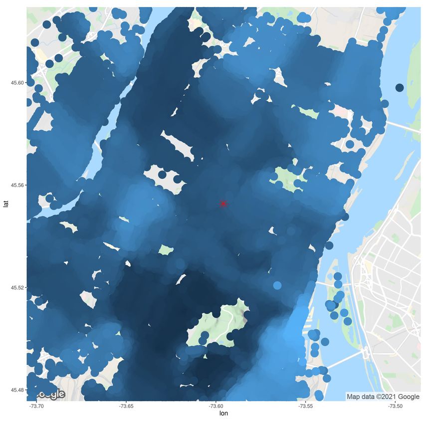
phenomena such as weather-based perils (flooding, hail, and storms) depend on natural factors
such as elevation and historic rainfall. Geographic ratemaking attempts to capture geographic
effects within the rating model. Historically, actuaries use spatial models to perform geographic
ratemaking.
    One may think that one must include a geographic component for a model to capture geographic
effects: either depending on coordinates or on indicator variables that identify a territory. Indeed,
the related research from actuarial science uses the latter approach. These models require a large
quantity of data to learn granular geographic effects and do not scale well to portfolios of large ter-
ritories. Until we model the geographic variables that generate the geographic risks, it is unfeasible
to model postal code level risk in a country-wide geographic model. In the present paper, we pro-
pose a method to construct geographic features that capture the relevant geographic information
to model geographic risk. We find that a model using these features as input to a GLM can model
geographic risk more accurately and more parsimoniously than previous geographic ratemaking
models.
    In this paper, we construct geographic features from census data. The intuition through this
paper is that since people generate risk, the geographic distribution of the population (as captured
by census data) relates to the geographic distribution of risk. For this reason, we place our emphasis
on constructing a model that captures the geographic distribution of the population, and use the
results from the population model to predict the geographic distribution of risk. If we capture the
geographic characteristics of the population correctly, then a ratemaking model using the geographic
distribution of the population as input may not require any geographic component (coordinate or
territory) since the geographic distribution of the population will implicitly capture some of the
geographic distribution of risk. We focus on the geographic distribution of populations as an
intermediate step of the predictive model. The main reason for this is that information about
populations is often free, publicly available and smooth, while information about risk is expensive,
private and noisy.

1.1   Spatial models

Spatial statistics is the field of science that studies spatial models. A typical problem in spatial
statistics is to sample continuous variables at discrete locations in a territory and predict the value
of this variable at another location within the same territory, called spatial interpolation. The
prevalent theory of spatial interpolation is regionalized variable theory, which assumes that we can
deconstruct a spatial random variable into a local structured mean, a local structured covariation,
and global unstructured variance (global noise) [Matheron, 1965, Wackernagel, 2013]. To compute
the pure premium of an insurance contract, it suffices to capture the local mean. Simple methods
like local averaging or bivariate smoothing (local polynomial regression or splines) can compute
this local mean.
   A very common spatial interpolation model is called kriging [Cressie, 1990], which performs
spatial interpolation with a Gaussian process parametrized by prior covariances. These covariances
depend on variogram models, a tool to measure spatial autocorrelation between pairs of points as a
function of distance. In our experience, variograms can be difficult to estimate in actuarial science
on claims data due to the large volume of zero observed losses.
   For risk management purposes, it is beneficial to study how geographic variables interact with
each other. For instance, one could study the distribution of losses for an insurance contract

                                                  2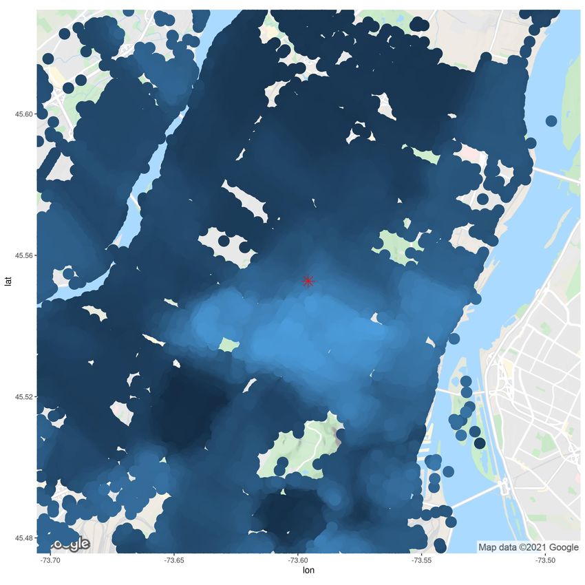
conditional on the fact that nearby policyholder incurred a loss. Spatial autocorrelation models
study the effect of nearness on geographic random variables [Getis, 2010]. Spatial autoregressive
models, which capture the spatial effects with latent spatial variables, are common approaches; see
[Cressie, 2015] for details.

1.2    Literature review

We now review the literature of geographic ratemaking in actuarial science. One can deconstruct
the spatial modeling process in three steps:
      step 1 data preparation and feature engineering;
      step 2 main regression model;
      step 3 smoothing model or residual correction.
Early geographic models in actuarial science were correction models that smoothed the residuals of a
regression model, i.e., capturing geographic effects after the main regression model, in a smoothing
model (step 3). Notable examples include [Taylor, 1989], [Boskov and Verrall, 1994] and [Taylor,
2001]. If we address the geographic effects during or before the main regression model, then the
smoothing step 3 is not required. [Dimakos and Di Rattalma, 2002] propose a Bayesian model that
captures geographic trend and dependence simultaneously to the main regression model, during
step 2. This model was later refined and studied as conditional autoregressive models by [Gschlößl
and Czado, 2007] and [Shi and Shi, 2017]. Another approach is spatial interpolation, that capture
geographically varying intercepts of the model. Examples include [Fahrmeir et al., 2003, Denuit
and Lang, 2004, Wang et al., 2017, Henckaerts et al., 2018], and other spatial interpolation methods
like regression-kriging [Hengl et al., 2007]. These methods use the geographic coordinates of the
risk along with multivariate regression functions to capture geographic trend.
    The above models capture geographic effects directly and non-parametrically, increasing model
complexity and making estimation difficult (increasing the number of parameters, making them
less competitive when comparing models based on criteria that penalize model complexity). As a
result, geographic smoothing methods adjusted on residuals step 3 are still the prevalent geographic
methods in practice for geographic ratemaking.
    In the present paper, we take a fundamentally different approach, capturing the geographic
effects during the feature engineering of step 1. Instead of capturing geographic effects non-
parametrically with geographic models, we introduce geographic data in the ratemaking model.
Geographic data is “data with implicit or explicit reference to a location relative to the Earth”
[ISO 19109, 2015]. Geographic data can describe natural variables describing the ecosystem and
the landform of a location, or artificial variables describing human settlement and infrastructure.
We study the effectiveness of automatically extracting useful representations of geographic infor-
mation with representation learning, see [Bengio et al., 2013] for a review of this field of computer
science.
   Early geographic representation models started with a specific application, then constructed
representations useful for their applications. These include [Eisenstein et al., 2010, Cocos and
Callison-Burch, 2017] for topical variation in text, [Yao et al., 2017] to predict land use, [Xu et al.,
2020] for user location prediction, and [Jeawak et al., 2019, Yin et al., 2019] for geo-aware prediction.
More recent approaches aim to create general geographic embeddings. These include [Saeidi et al.,
2015], who use principal component analysis and autoencoders to compress census information.

                                                   3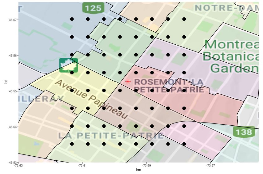
In [Fu et al., 2019], [Zhang et al., 2019] and [Du et al., 2019], the authors use point-of-interest
and human mobility data to construct spatial representations of spatial regions in a framework
that preserves intra-region geographic structures and spatial autocorrelation. The authors use
graph convolutional neural networks to train the representations. In [Jenkins et al., 2019], the
authors propose a method to create representations of regions using satellite images, point-of-
interest, human mobility and spatial graph data. Then, [Blier-Wong et al., 2020] propose a method
that captures the geographic nature of data into a geographic data cuboid, using convolutional
neural networks to construct representations using Canadian census information. The proposed
model is coordinate-based, therefore more flexible than regions. [Hui et al., 2020] use graphical
convolutional neural networks to compress census data in the United States to predict economic
growth trends. Finally, [Wang et al., 2020] propose a framework to learn neighborhood embeddings
from street view images and point-of-interest data.

2     Spatial representations

In [Blier-Wong et al., 2021a], we propose a framework for actuarial modeling with emerging sources
of data. This approach separates the modeling process into two steps: a representation model and
a predictive model. Using this deconstruction, we can leverage modern machine learning models’
complexity to create useful representations of data and use the resulting representations within a
simpler predictive model (like a generalized linear model, GLM). This section presents an overview
of representation models, with a focus on spatial embeddings.

2.1    Overview of representation models

The defining characteristic of a representation model (as opposed to an end-to-end model) is that
representation models never use the response variable of interest during training, relying instead
on the input variables themselves or other response variables related to the insurance domain. We
propose using encoder/decoder models to construct embeddings, typically with an intermediate
representation (embedding) with a smaller dimension than the input data; see Figure 1 for the
outline of a typical process. When training the representation model, we adjust the parameters of
the encoder and the decoder, two machine learning algorithms. To construct the simpler regression
model (like a GLM), one extracts embedding vectors for every observation and stores them in a
design matrix.

        Input              Encoder            Embedding              Decoder            Output

                                                                 Predictive model

                               Figure 1: Encoder/decoder architecture

    The representation construction process has four steps:
      step 1 Construct an encoder, transforming input variables into a latent embedding vector.
      step 2 Construct a decoder, which will determine which information the representation model
             must capture.

                                                 4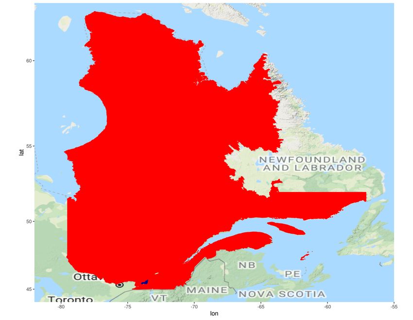
step 3 (Optional) Combine features from different sources into one combined embedding.
      step 4 (Optional) Evaluate different embeddings, validate the quality of representations.
We now enumerate a few general advantages of the representation approach. First, representation
models can transform categorical variables into dense and compact vectors, which is particularly
important for territories since the cardinality of this category of variables is typically very large.
Second, representation models can reduce the input variable dimension into one of our choosing:
we typically select an embedding dimension much smaller than the original. Third, we can build
representations such that they are useful for general tasks, so we can reuse representations. Fourth,
representations can learn non-linear transformations and interactions automatically, eliminating
the need to construct features by hand. Finally, when using a representation model, one can reduce
the regression model’s complexity. If the representation model learns all useful interactions and
non-linear transformations, a simple model like a GLM could replace more complex models like
end-to-end gradient boosting machines or neural networks.

2.2     Motivation for geographic embeddings

The geographic methods proposed in actuarial science (see the literature review) address the data’s
geographic nature at step 2 and step 3 of geographic modeling. Geographic embeddings are a
fundamentally different approach to geographic models studied in actuarial science. We first trans-
form geographic data into geographic embedding vectors, during feature engineering (step 1). By
using geographic embeddings in the main regression model, we capture the geographic effects and
the traditional variables at the same time. Figure 2 provides an overview of the method. The
representation model takes geographic data as input to automatically create geographic features
(geographic embeddings). Sections 3 and 4 respectively present architectures and implementations
of geographic embedding models. Then, we combine the geographic embeddings with other sources
of data (for example, traditional actuarial variables like customer age). Finally, we use the combined
feature vector within a predictive model.

  Traditional variables x   Traditional features x∗

                                                           Concatenated features     Predictive model         Prediction

  Geographic variables γ    Geographic features   γ∗

                                        step 1: representation model               step 2: predictive model

                             Figure 2: Proposed geographic ratemaking process

    The representation model’s complexity does not affect the predictive model’s since the represen-
tation model is unsupervised with respect to the predictive task. We can construct representation
models that are highly non-linear with architectures that capture the unique characteristics of dif-
ferent data sources. This model will induce geographic effects into embeddings while capturing
the desirable characteristics of geographic models. In most cases, regression models (GLMs) using
these geographic embeddings as inputs will have lower variance and often lower bias than geographic
models, as demonstrated with examples in Section 5.
    In [Blier-Wong et al., 2021a], the authors present a collection of tools to construct useful ac-

                                                                       5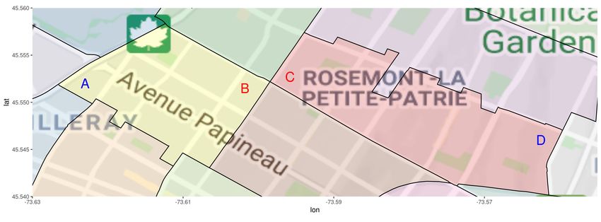
tuarial representations. Section 7 of that paper deals with geographic representation ideas. The
present paper aims to pursue our investigation on geographic representations for actuarial science
by providing an implementation and an application.
     The representation learning framework enables one to select an architecture that captures spe-
cific desirable attributes from various data sources. There is one generally accepted desirable
attribute for geographic models, called Tobler’s first law (TFL) of geography. We also propose
two new attributes that make geographic embeddings more useful, based on our experience with
geographic models. Below is a list of these three desirable attributes for geographic embeddings.

Attribute 1 (TFL) Geographic embeddings must follow Tobler’s first law of geography. As men-
tioned in [Tobler, 1970], “everything is related to everything else, but near things are more related
than distant things”. This attribute is at the core of spatial autocorrelation statistics. Spatial au-
tocorrelation is often treated as a confounding variable, but these variables constitute information
since it captures how territories are related (see, e.g., [Miller, 2004] for a discussion). A represen-
tation model, capturing the latent structure of underlying data, generates geographic embeddings.

Attribute 2 (coordinate) Geographic embeddings are coordinate-based. A coordinate-based model
depends only on the risk’s actual coordinates and its relation to other coordinates nearby. Polygon-
based models highly depend on the definition of polygon boundaries, which could be designed for
tasks unrelated to insurance.
    We motivate this attribute with an example. Consider four customers A, B, C and D, that have
home insurance for their house in the island of Montréal, Québec, Canada. Figure 3 identifies each
coordinate on a map. We also included the borders of polygons, represented by bold black lines.
These polygons correspond to Forward Sortation Areas (FSA), a unit of geographic coordinate in
Canada (further explained in Section 4). Observations A and B belong to the same polygon, while
observations B and C belong to different ones. However, B is closer to C than to A. Polygon-based
representation models and polygon-based ratemaking models assume that the same geographic
effect applies to locations A and B, while different geographic effects apply to locations B and C.
However, following TFL, one expects the geographic risk between customers B and C to be more
similar than the geographic risk between A and B.
    There are two other issues with the use of polygons. The first is that the actual shapes of
polygons could be designed for purposes that are not relevant for capturing geographic risk (for
example, postal codes are typically optimized for mail distribution). If an insurance company
uses polygons for geographic ratemaking, it is crucial to verify that risks within each polygons are
geographically homogeneous. The second issue is that polygon boundaries may change in time. If
postal codes are split, moved, merged or created, the geographic ratemaking model will also split,
move, merge the territories, and be unable to predict for newly created postal codes. A customer
living at the same address could see its insurance premium drastically increase or decrease due to
the arbitrary change in polygon boundary, even if there is no actual change in the geographic risk.
    Finally, the type of location information (coordinate or polygon) for the ultimate regression
task may be unknown while training the embeddings. For this reason, one should not make the
polygon depend on a specific set of boundary polygon shapes. On the other hand, one can easily
aggregate coordinates into the desired location type for the ultimate regression task.

Attribute 3 (external) Geographic embeddings encode relevant external information. There are
two reasons for using external information. The first is that geographic effects are complex, so we

                                                  6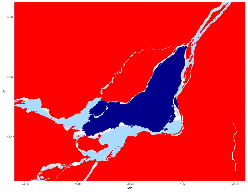
Figure 3: Coordinates vs polygons

need a large volume of geographic information to capture the confounding variable that generates
them. Constructing geographic embeddings with a dataset external to one’s specific problem may
increase the quantity and quality of data, providing new information for spatial prediction. The
second reason is that geographic embeddings can produce rates in territories with no historical loss
experience, as long as we have external information for the new territory. Traditional geographic
models capture geographic effects from experience but are useless to rate new territories. If we train
geographic embeddings on external datasets that cover a wider area than the loss experience of an
insurance company, we may use the geographic embeddings to capture geographic effects in territo-
ries with no loss experience. This second reason is related to using one-hot encodings of territories;
see [Blier-Wong et al., 2021a] for further illustrations. Finally, the external information should
be relevant to the insurance domain. Although geographic embeddings could be domain agnostic
(general geographic embeddings for arbitrary tasks), our ultimate goal is geographic ratemaking,
so we select the external information that is related to causes of geographic risks.

    To construct the geographic representations, we use a flexible family of machine learning meth-
ods called deep neural networks. In the past few years, actuarial applications of neural networks
are increasing in popularity; see [Richman, 2020, Blier-Wong et al., 2021b] for recent reviews. We
construct the neural networks such that the representations satisfy the three desirable attributes of
geographic embeddings, so any predictive model (even linear ones) using the geographic embeddings
as input will also satisfy the desirable attributes.

2.3   Relationship with word embeddings

The geographic embeddings approach that we propose is largely inspired by word embeddings
in natural language processing (NLP). The fundamental idea of word embeddings dates back to
linguists in the 1950’s. On the subject of the distributional hypothesis and synonyms, [Harris,
1954] states “If A and B have some environments in common and some not . . . we say that they
have different meanings, the amount of meaning difference corresponding roughly to the amount
of difference in their environments.” Although this environment refers to the context of a word
within text, this same quote applies to geography. Another justification that resembles TFL comes
from [Firth, 1957], stating “You shall know a word by the company it keeps!”
    Words and territories are also similar since one represents them as categorical variables with a
large cardinality. For this reason, it isn’t surprising that the classical models for NLP tasks and
geographic prediction are similar. Simple representations of text like bag-of-words and n-grams

                                                  7
are similar to simple representations of territories like one-hot encodings. Further techniques use
smoothing to account for unknown words or territories, while more sophisticated methods use
graphical models like hidden Markov models or conditional autoregressive models to account for
textual or geographic autocorrelation. Most recent models in NLP use word embeddings [Mikolov
et al., 2017], and researchers are starting to study geographic embeddings. Table 1 summarizes the
comparisons outlined in this paragraph.
NLP Geography
Distributional hypothesis Tobler’s first law of geography
Fondamental justification [Harris, 1954, Firth, 1957] [Tobler, 1970]
Bag-of-words & n-grams One-hot encoding of territories
Classical tools & techniques n-gram smoothing (Laplace) Smoothing (kriging, splines)
Hidden Markov models Conditional autoregressive models
Word embeddings Geographic embeddings
Representation techniques [Mikolov et al., 2013] [Fu et al., 2019],
[Devlin et al., 2019] [Blier-Wong et al., 2020]
Table 1: Comparing contributions and techniques for NLP and geographic models
Attribute 2 proposes to use coordinates instead of polygons to construct geographic embeddings.
This is analogous to using character-level embeddings instead of word embeddings. NLP researchers
use character-level embeddings to understand the semantics of an unknown word (a word which we
never saw in a training corpus).
The principal difference between words and territories is that territories are not interchangeable
or synonymous. Instead, we capture the co-occurrence of relevant geographic information, see
attribute 3.
3 Convolution-based geographic embedding model
In this section, we describe an approach to construct geographic embeddings. We will explain the
representation model choices for the encoder in step 1, the decoder in step 2 and the evaluation in
step 4. For the embeddings to have all desirable attributes of geographic embeddings enumerated
in the previous section, we must modify the process to account for geographic data, adding a data
preparation step. Our focus is on constructing a geographic representation model, so we omit the
(optional) step 3 of combining representations with other sources of data in this section.
3.1 Preparing the data
Suppose we are interested in creating a geographic feature that characterizes a location s. Fol-
lowing attribute 3 (external), we must first collect geographic information for location s. Objects
characterized by their location in space can be stored as point coordinates or polygons (boundary
coordinates) [Anselin et al., 2010]. Point coordinate data corresponds to the measurements of a
variable at an individual location. It can indicate the presence of a phenomenon (set of locations
where accidents occurred) or the measurement of a variable at a particular location (age of a build-
ing at a location) [Diggle, 2013]. Polygon data aggregates variables from all point patterns in a
8territory. In Figure 3, the individual marks A, B, C and D are point patterns, and the different
shaded areas are polygons.
To construct the representation model, we assume that we have one or many external datasets
in polygon format, with a vector of data for each polygon. This is the case for census data in
North America. Suppose the coordinate of s is located within the boundaries of polygon S, then
one associates the external geographic data from polygon S to location s. We will use the notation
γ ∈ Rd to denote the vector of geographic variables.
In usual (non-spatial) situations, the type and format of data determines the topology of the
encoder. Geographic information is often vectorial (called spatial explanatory variables [Diggle and
Ribeiro, 2007]) so that the associated neural network encoder would be a fully-connected neural
network. A fully-connected neural network encoder would satisfy the external attribute, but not
TFL or coordinate. To understand why the coordinate is not entirely satisfied, we consider one
external data source from one set of polygons. In this case, observations within the same polygon
will have the same geographic variables γ, so the geographic data remains polygon-based. Instead,
we modify the input data for the representation model to satisfy the TFL and coordinate attributes.
To create an embedding of location s, we will not only use information from location s, but also data
from surrounding locations. Since each coordinate within a polygon may have different surrounding
locations, the resulting embeddings will not be polygon-based, satisfying the coordinate attribute.
An approach to satisfy TFL is to use an encoder that includes a notion of nearness. Convolu-
tional neural networks (CNNs) have the property of sparse interactions, meaning the outputs of a
convolutional operation are features that depend on local subsets of the input [Goodfellow et al.,
2016]. CNNs accept matrix data as input. For this reason, we will define our neighbors to form a
grid around a central location. The representation model’s input data is the geographic data square
cuboid from [Blier-Wong et al., 2020], which we present in Algorithm 1 and explain below. One
notices that the geographic data square cuboid is a specific case of a multiband raster, datacube
or multidimensional array.
To create the geographic data cuboid for a location s with coordinate (lon, lat), we span a grid
of p × p neighbors, centered around (lon, lat). Each neighbor in the grid is separated horizontally
and vertically by a distance of w. The steps 1 to 4 of Algorithm 1 create the matrix of coordinates
for the neighbors, and we illustrate each transformation in Figure 4. w
1
w
w
(a) Unit grid (b) Scale (c) Rotate (d) Translate
Figure 4: Creating the grid of neighbors
Each coordinate in δ has geographic variables γ ∈ Rd , extracted from different external data
sources of polygon data. The set of variables for every location in δ, which we note γ δ , forms
a square cuboid of dimension p × p × d, which we illustrate in Figure 6. We can interpret the
geographic data square cuboid as an image with d channels, with one channel for each variable.
Algorithm 1 presents the steps to create the data square cuboid for a single location. Lines 1 to
9Algorithm 1: Generating a geographic data square cuboid
Input: Center coordinate (lon, lat), width w, size p, geographic data sources
Output: Geographic data square cuboid
1 generate empty grid of dimension p × p and width 1 with the set
p−1
[ p−1
[
1 1
(2k − p + 1) , (2j − p + 1) ,
2 2
k=0 j=0
store the coordinates of this set of points in a matrix δ0 (each column is a coordinate, the
first row is the longitude, the second row is the latitude);
2 scale (multiply) by w;
cos θ − sin θ
3 sample θ ∼ U nif (0, 360) and rotate the scaled matrix, R(wδ0 ) = w δ0 ;
sin θ cos θ
lon
4 translate matrix by (lon, lat)0 , to get δ = R(wδ0 ) + ;
lat
5 foreach external geographic data source do
6 foreach coordinate in δ do
7 allocate coordinate to corresponding polygon index;
8 append vector data to current coordinate
4 generate the set δ for the center location (the matrix of neighbor coordinates), while lines 4 to
7 fill each coordinate’s variables. The random rotation is present such that our model does not
exclusively learn effects in the same orientation.
Variable d
Variable d-1
Variable 3
Variable 2
Variable 1
Figure 5: Set of neighbor coordinates δ Figure 6: Data square cuboid γ δ
If the grid size p is even, δ does not include the center coordinate (lon, lat). This means the
geographic data square cuboid depends only on neighbor information and not information of the
center point itself.
103.2 Constructing the encoder
As explained in Section 2.1, the encoder generates a latent representation from a bottleneck, which
we then extract as embeddings. Above, we constructed the input data to have a square cuboid shape
to use convolutional neural networks as an encoder. The encoder has convolutional operations,
reducing the size of the hidden square cuboids (also called feature maps in computer vision) after
each set of convolutions. Then, we unroll (from left to right, top to bottom, front to back, see
Figure 7 for an illustration) the square cuboid into a vector. The unrolled vector will be highly
autocorrelated: since the output of the convolutions includes local features, features from the same
convolutional layer will be similar to each other, causing collinearity if we use the unrolled vector
directly within a GLM. For this reason, we place fully-connected layers after the unrolled vector.
The last fully-connected layer of the encoder is the geographic embedding vector, noted γ ∗ . This
layer typically has the smallest dimension of the entire neural network representation model. For
a geographic embedding of dimension `, then the encoder will be a function Rp×p×d → R` .
e f
a bg unroll
c d
h
= a b c d e f g h
Figure 7: Unrolling example for a 2 × 2 × 2 cuboid. Different colors are different variables
We have now constructed the encoder for our representation model. This encoder satisfies
desirable attributes 1 to 3 since
1. the encoder is a convolutional neural network, which captures sparse interactions from neigh-
boring information, encoding the notion of nearness;
2. the embeddings are coordinate-based: as the center coordinate moves, the neighboring coordi-
nates also move, so center coordinates within the same polygon may have different geographic
data square cuboids;
3. the model uses external data as opposed to one-hot encodings of territories.
3.3 Constructing the decoder
The decoder guides the type of information that the embeddings encode, i.e., selects which domain
knowledge to induce into the representations, see Section 2.1 for details on the decoding procedure.
If one has response variables related to the insurance domain for the whole dataset (i.e., for all
coordinates within the territory for which we construct embeddings), we could train the decoder
with transfer learning, such that the representation model learns important information related to
insurance. In our case, the external dataset that covers Canada, and we do not have insurance
statistics over the entire country. For this reason, our decoder will attempt to predict itself, i.e.,
the input variables γ.
The original model for geographic embeddings we explored was the convolutional regional au-
toencoder (CRAE), presented in [Blier-Wong et al., 2020]. The input of CRAE is the geographic
data cuboid, and the output is also the geographic data cuboid. The neural network architecture
is called a convolutional autoencoder since the model’s objective is to reconstruct the input data
after going through a bottleneck of layers. The decoder in CRAE is a function R` → Rp×p×d . One
11can interpret CRAE as using contextual variables to predict the same contextual variables. The loss
function for CRAE is the average reconstruction error. For a dataset of N coordinates, the loss
function is
N
1 X 2
L= g f γδ − γδ , (1)
N i i
i=1
where f is the encoder, g is the decoder, γ δ ∈ Rp×p×d is the geographic data cuboid for the coor-
i
dinate of location i and || · || is the euclidean norm. However, attribute 2 only requires information
from the grid’s central location, not the entire grid. Therefore, much of the information contained
within CRAE embeddings captures irrelevant or redundant information.
In this paper, we improve CRAE by changing the decoder. One can interpret the new model as
using contextual variables to predict the central variables, directly satisfying the coordinate attribute.
This same motivation was suggested for natural language processing in [Collobert and Weston, 2008]
and applied in a model called Continuous Bag of Words (CBOW) [Mikolov et al., 2013]. Instead
of reconstructing the entire geographic data cube, the decoder attempts to predict the variables γ
for location s. Therefore, the decoder is a series of fully-connected layers that act as a function
R` → Rd , where `
d. The loss function for CBOW-CRAE is also the average reconstruction
error, but on the vector of variables for the central location instead on the entire geographic data
square cuboid:
N
1 X 2
L= g f γδ − γi . (2)
N i
i=1
Figure 8 illustrates the entire convolution-based model architecture of CBOW-CRAE.
g
in
dd
be
Em
t
pu
l
ut
ol
nr
O
t
U
pu
In
Figure 8: Convolution-based geographic embedding model
3.4 Evaluating representations
There are two types of evaluations for embeddings: the most important are extrinsic evaluations,
but intrinsic evaluations are also significant [Jurafsky and Martin, 2009]. One evaluates embeddings
extrinsically by using them in downstream tasks and comparing their predictive performance. In
P&C actuarial ratemaking, one can use the embeddings within ratemaking models for different
lines of business and select the embedding model that minimizes the loss on out-of-sample data.
According to our knowledge, there are no intrinsic evaluation methods for geographic embed-
dings. We propose one method in this paper and discuss other approaches in the conclusion.
Intrinsic evaluations determine if the embeddings behave as expected. To evaluate embeddings
intrinsically, one can determine if they possess the three attributes proposed in Section 2. Due to
12the geographic data cuboid construction, geographic embeddings already satisfy attributes coordi-
nate and external, so these attributes do not need intrinsic evaluations. To validate TFL, we can
plot individual dimensions of the embedding vector on a map. Embeddings that satisfy TFL vary
smoothly, and one can inspect this property visually. Section 4.7 presents the implicit evaluation
for the implementation on Canadian census data.
4 Implementations of geographic embeddings
In this section, we present an implementation of geographic embeddings using census data in
Canada. We select census data since they contain crucial socio-demographic information on the
customer’s geography; geographic embeddings trained with census data will compress this informa-
tion. One could also use natural (ecosystem, landform, weather) information to create geographic
embeddings that capture natural geographic risk. We first present the census data in Canada,
along with issues related to some of its characteristics. Then, we explain the architectural choices
and implementations for the geographic data square cuboid, the encoder and the decoder. Finally,
we perform intrinsic evaluations of the geographic embeddings.
Our strategy for constructing geographic embeddings contains two types of hyperparameters:
general neural network hyperparameters, and specific hyperparameters related to the particular
model architecture. General hyperparameters control the method used to optimize the neural net-
work parameters, especially the optimization routine: these include the choice of the optimizer,
the batch size, the learning rate, the weight decay, the number of epochs and the patience for the
learning rate reduction. We select general hyperparameters using grid-search, along with personal
experience with neural networks. We refer the reader to other texts such as [Goodfellow et al.,
2016] for general tips on hyperparameter search. We will limit our discussion of general hyperpa-
rameter search to mentioning the optimal parameters that we use. Specific hyperparameters are
associated with the specific neural network architecture and includes the square cuboid width w
and the pixel size p to generate a geographic data square cuboid. Other specific hyperparameters
determine the neural network architecture, including the shape and depth of convolutions and fully
connected layers. Tuning these hyperparameters requires experience with neural networks since the
combinations of specific hyperparameters are much too large to determine using grid-search. We
will explain our thought process: starting with accepted heuristics, then manually exploring the
hyperparameter space to determine the optimal architecture.
4.1 Canadian census data
We now present some characteristics of Canadian census data. Statistics Canada publishes this
data every five years, and our implementation uses the most recent version (2016). The data
is aggregated into polygons called forward sortation areas, which correspond to the first three
characters of a Canadian postal code; see Figure 9 for the decomposition of a postal code. Statistics
Canada aggregates the public release of census data to avoid revealing confidential and individual
information. The data is also available at the dissemination area polygon level, which is more
granular than FSA. We work with FSAs because they are simpler to explain. There are 1 640
FSAs in Canada, and each polygon in Figure 5 represents a different FSA. The grid of neighbor
coordinates of Figure 5 contains 8 points from the same FSA as the central location, represented
by the red star.
13Postal district
H2T 1W8
FSA LDU
Figure 9: Deconstruction of a Canadian postal code
The first issue with using census data for insurance pricing is the use of protected attributes, i.e.,
variables that should legally or ethically not influence the model prediction. One example is race
and ethnicity [Frees, 2015]. Territories may exhibit a high correlation with protected attributes like
ethnic origin. To construct the geographic embeddings, we discard all variables related to ethnic
origin (country of origin, mother tongue, citizen status). We retrain only variables that a Canadian
insurance company could use for ratemaking. In Appendix A, we provide a complete list of the
categories of variables within the census dataset, and we denote with an asterisk the categories
of variables that we omit. What remains is information about age, education, commute, income
and others, and comprises 512 variables that we denote γ. Removing protected attributes from a
model is a technique called anti-classification [Corbett-Davies and Goel, 2018], or fairness through
unawareness [Kusner et al., 2018], which does not eliminate discrimination entirely and in some
cases may increase it [Kusner et al., 2018]. Studying discrimination-free methods to construct
geographic embeddings is kept as future work. For analysis and discussion of discrimination in
actuarial ratemaking, see [Lindholm et al., 2020].
It is common practice in machine learning to normalize input variables such that they are all on
the same scale. Two reasons are that stochastic gradient-based algorithms typically converge faster
with normalized variables, and un-normalized variables have different impacts on the regularization
terms of the loss function [Shalev-Shwartz and Ben-David, 2014]. For autoencoders, an additional
reason is that the model’s output is the reconstruction of many variables, so variables with a higher
magnitude will generate a disproportionately large reconstruction error relative to other variables
(so the model will place more importance on reconstructing these variables). Normalization re-
quires special attention for aggregated variables like averages, medians, and sums: some must be
aggregated with respect to a small number of observations, others with respect to the population
within the FSA of interest and others with the Canadian average. For example, the FSA population
is min-max normalized (see [Han et al., 2011]) with respect to all FSAs in Canada. For age group
proportions (for instance, the proportion of 15 to 19-year-olds), we normalize with respect to the
current FSA’s population size.
When using Algorithm 1, some coordinates do not belong to a polygon index, which happens
when the coordinate is located in a body of water. To deal with this situation, we created a vector
of missing values filled with the value 0.
Finally, we project all coordinates to Atlas Lambert [Lambert, 1772, Snyder, 1987] to reduce
errors when computing distances. Due to Earth’s curvature, computing Euclidean distance with
degree-based coordinates like GPS underestimates distances; see [Torge and Müller, 2012] for il-
lustrations. When changing the coordinate system to Atlas Lambert, one can compute distances
using traditional euclidean metrics with greater accuracy.
144.2 Geographic data square cuboid
Now that we have prepared the census data, we can construct the geographic data cuboid for our
implementation. The parameters for the geographic data square cuboid include square width w and
pixel size p. One can interpret these values as smoothing parameters. The square width w affects
the geographic scale of the neighbors, while the pixel size p determines the density of the neighbors.
For very flexible embeddings, one can choose small w so that the geographic embeddings will capture
local geographic effects. If the embeddings are too noisy, then one can increase p to stabilize the
embedding values. Ultimately, the importance is the span of the grid, determined by the farthest
sampled neighbors. For an even value of w, the closest sampled√ neighbor coordinates are the four
corners surrounding the central location at a distance of p/ 2 units from the central location. The
√
farthest sampled neighbors are the four outermost corners of the grid at a distance of p(w − 1)/ 2
units. Selecting the best parameters is a tradeoff between capturing local variations in densely
populated areas and smoothing random fluctuations in rural areas. Insurance companies could
construct embeddings for rural portfolios and urban portfolios with different spans to overcome this
compromise. Another solution consists of letting the parameters depend on local characteristics of
the population, such as population density (select parameters such that the population contained
within a grid is above a threshold) or the range of a variogram (select parameters such that the
observations within the grid still exhibit geographic autocorrelation).
We consider square widths of w = {8, 16} and pixel sizes of p = {50, 100, 500} meters. Our
experiments showed that a square width of w = 16 and a pixel size of p = 100 meters produced
smaller reconstruction errors. The geographic data square cuboid then samples 162 = 256 neigh-
bors, the closest one being at a distance of 71 meters and the farthest one at 1061 meters from the
center location. Since we have 512 features available for every neighbor, the size of the input data
is 16 × 16 × 512 and contains 131 072 values.
The dataset used to train the representation models is composed of a geographic data square
cuboid for every postal code in Canada (888 533 by the time of our experiments). A dataset
containing the values of every geographic data square cuboid would take 2To of memory, too large
to hold in most personal computers. For this reason, we could not generate the complete dataset.
However, one can still train geographic embeddings on a personal computer by leveraging the fact
that many values in the dataset repeat. For each postal code, one generates the grid of neighbor
coordinates (steps 1 to 4 of Algorithm 1) and identifies the corresponding FSA for each coordinate
(step 6 of Algorithm 1). We then unroll the grid from left to right and from top to bottom into
a vector of size 256. For memory reasons, we create a numeric index for every FSA (A0A = 1,
A0B = 2, . . . , Y1A = 1 640), and store the list of index for every postal code in a CSV file (1GB).
Another dataset contains the normalized geographic variables γ for every FSA (15.1MB). Most
modern computers can load both datasets in RAM. During training, our implementation retrieves
the vector from the index and retrieves the values associated with each FSA (step 8 of Algorithm
1), then rolls the data into geographic data square cuboids.
4.3 Encoders
This subsection will detail specific architecture choices for encoders with Canadian census data,
presenting two strategies to determine the optimal architecture. Each contains two convolution
layers with batch normalization [Ioffe and Szegedy, 2015] and two fully-connected layers. Strategy 1
reduces the feature size between the last convolution layer and the first fully-connected layer, while
15strategy 2 reduces the feature size between convolution layers. Each encoder uses a hyperbolic
tangent (tanh) activation function after the last fully-connected layer to constrain the embedding
values between -1 and 1. After testing convolutional kernels of size k = {3, 5, 7}, the value k = 3
resulted in the lowest reconstruction errors.
4.3.1 Strategy 1
A popular strategy for CNN architectures is to reduce the width and height but increase the depth
of intermediate features as we go deeper into the network, see [Simonyan and Zisserman, 2014, He
et al., 2016]. The first strategy follows three heuristics:
1. Apply half padding, such that the output dimension of intermediate convolution features
remains the same.
2. Apply max-pooling after each convolution step with a stride and kernel size of 2, reducing
the feature size by a factor of 4.
3. Double the square cuboid depth after each convolution step.
The result of this strategy is that the size (the number of features in the intermediate representa-
tions) is reduced by two after every convolution operation. We present the square cuboid depth and
dimension at all stages of the models in Table 2. The feature size (row 3) is the product of square
cuboid depth (number of channels) and the dimension of the intermediate features. In strategy 1,
Input Conv1 Conv2 Unroll FC1 FC2
Square cuboid depth 512 1 024 2 048 32 768 128 16
Square cuboid width × height 16 × 16 8×8 4×4 1 1 1
Feature size 131 072 65 536 32 768 32 768 128 16
% of parameters NA 17 68 NA 15 0
Table 2: Large encoder model with 27 798 672 parameters
the convolution step accounts for most parameters. The steepest decrease in feature size occurs
between the second convolution block and the first fully-connected layer (from 32 768 to 128).
4.3.2 Strategy 2
For the second strategy, we follow a trial and error approach and attempt to restrict the number of
parameters in the model. We retain heuristics 1 and 2 from strategy 1, but the depth of features
decrease between each convolution block.
Input Conv1 Conv2 Unroll FC1 FC2
Square cuboid depth 512 48 16 256 16 8
Square cuboid width × height 16 × 16 8×8 4×4 1 1 1
Feature size 131 072 3 072 256 256 16 8
% of parameters NA 95 3 NA 2 0
Table 3: Small encoder model with 232 514 parameters
In strategy 2, 95% of the parameters are in the first convolution step. The feature size decreases
steadily between each operation.
164.4 CRAE & CBOW-CRAE decoders
The output for the CRAE model is the reconstructed geographic data cuboid. The decoder in
this model is the inverse operations of the encoder (deconvolutions and max-unpooling). The final
activation function is sigmoid because the original inputs are between 0 and 1. We present the
decoder operations for the large and the small decoders in Tables 4 and 5. Recall that the input
to the decoder is the embedding layer from the encoder.
Input FC3 FC4 Roll Deconv1 Deconv2
Square cuboid depth 16 128 32 768 2 048 1 024 512
Square cuboid width × height 1 1 1 4×4 8×8 16 × 16
Feature size 16 128 32 768 32 768 65 536 131 072
% of parameters NA 0 15 NA 68 17
Table 4: Large CRAE decoder model
Input FC3 FC4 Roll Deconv1 Deconv2
Square cuboid depth 8 16 256 16 48 512
Square cuboid width × height 1 1 1 4×4 8×8 16 × 16
Feature size 8 16 256 256 3 072 131 072
% of parameters NA 91 3 NA 2 0
Table 5: Small CRAE decoder model
The CBOW-CRAE is a context to location model, so we select a fully-connected decoder,
increasing from the embedding (γ ∗ ) size ` to the geographic variable (γ) size d. In our experience,
the decoder’s exact dimensions did not significantly impact the reconstruction error, so we select
the ascent dimensions (FC3 and FC4) to be the same as the fully-connected descent dimensions
(FC1 and FC2). When there is no hidden layer from the embedding to the output (if there is only
one fully-connected layer), the model is too linear to reconstruct the input data. When there is
one hidden layer, the model is mainly able to reconstruct the data. Additional hidden layers did
not significantly reduce the reconstruction error, so we select only one hidden layer in the decoder.
Table 6 presents the CBOW CRAE decoders in our implementation.
Input FC3 FC4
Small model 8 16 512
Large model 16 128 512
Table 6: CBOW-CRAE decoders
4.5 Comments on general hyperparameters and optimization strategy
We now offer a few comments on the training strategy. We split the postal codes into a training
set and a validation set. Since the dataset is very large, we select a test set composed of only 5%
of the postal codes. We train the neural networks on a GeForce RTX 2080 8 GB GDDR6 graphics
card and present the approximate training time later in this section. The batch size is the largest
17power of 2 that fits on the graphics card. We train the neural networks in PyTorch [Paszke et al.,
2019] with the Adam optimization procedure from [Kingma and Ba, 2014]. We do not use weight
decay (L2 regularization) since the model does not overfit. The initial learning rate for all models
is 0.001 and decreases by a factor of 10 when losses stop decreasing for ten consecutive epochs.
After five decreases, we stop the training procedure.
The most significant issue during training is the saturation of initial hidden values (see, e.g.,
[Glorot and Bengio, 2010] for a discussion of the effect of neuron saturation and weight initializa-
tion). The encoder and the decoder’s output are respectively tanh and sigmoid activations, which
have horizontal asymptotes and small derivatives for high magnitude inputs. All models use batch
normalization, without which the embeddings saturate quickly. Initializing the network with large
weights, using the techniques from [Glorot and Bengio, 2010], generated saturated embedding val-
ues of -1 or 1. To improve training, we initialize our models with very small weights, such that the
average embedding value has a small variance and zero-centered. The neural network gradually
increases the weights, so embeddings saturate less.
The activation functions for intermediate layers are hyperparameters; we compare tanh and
rectified linear unit (ReLU). The ReLU activation function generated the best performances, but
the models did not converge for every initial seed. Our selected models use ReLU, but sometimes
required restarting the training process with a different initial seed if the embeddings saturate.
4.6 Training results
In this section, we provide results on the implementations of the four geographic embedding ar-
chitectures, along with observations. Table 7 presents the training and validation reconstruction
errors, along with the training time, the number of parameters and the mean embedding values.
Training MSE Validation MSE Time Parameters Mean value
Small CRAE 0.21299473 0.21207126 5 hours 465 688 0.2051166
Large CRAE 0.21088413 0.20995240 3 days 55 622 416 0.6909323
Small CBOW-CRAE 0.21833613 0.21715157 2 hours 241 384 0.3463651
Large CBOW-CRAE 0.21731463 0.21609975 2 days 27 866 896 0.1174563
Table 7: Reconstruction errors from architectures
One cannot directly compare the reconstruction errors for the classic CRAE and CBOW-CRAE
since classic CRAE reconstructs p2 as many values as CBOW-CRAE. The average reconstruction
error for CRAE is smaller than for CBOW-CRAE, which could be because the output of CBOW-
CRAE does not have a determined equivalent vector in the input data. The CRAE model attempts
to construct a one-to-one identity function for every neighbor because the input is identical to the
output. On the other hand, CBOW-CRAE cannot exactly predict the values for a specific neighbor
in the grid since there is no guarantee that the specific neighbor belongs to the same polygon as the
central coordinate. One also notices that the validation data’s reconstruction error is smaller than
the training data, which is atypical in machine learning. However, changing the initial seed for
training and validation data changes this relationship, so one attributes this effect to the specific
data split. This also means that the model does not overfit on the training data: if it did, then
the training error would be much smaller than the validation error. The lack of overfit is a result
of the bottleneck dimension being small (8 or 16 dimensions) with respect to the dimension of the
18input data (131 072).
For space and clarity reasons, we will not perform the explicit and implicit evaluations of
embeddings. We do not find that one set of embeddings always performs better than the others,
but find that the Large CBOW-CRAE behaves more appropriately, even if the reconstruction error
is worse than for CRAE model. First, the average embeddings values for CBOW-CRAE models
are closer to 0, which is desirable to increase the representation flexibility (especially within a
GLM, because the range of embeddings is [-1, 1]). Attempts to manually correct these issues
(normalization of embedding values after training) do not improve the quality of embeddings. In
addition, the Large CBOW-CRAE had less saturated embedding dimensions, as we will discuss
in the implicit evaluations. For these reasons, we continue our evaluation of embeddings with the
Large CBOW-CRAE model, but we encourage researchers to experiment with other configurations.
4.7 Implicit evaluation of embeddings
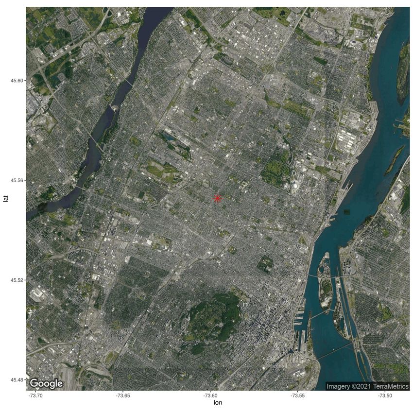
We now implicitly evaluate if the 16 dimensions of the embeddings (generated by the Large CBOW-
CRAE model) follows attribute 1 (TFL). Figure 10 presents an empty map for a location in Montréal
(to identify points of interest), along with two embedding dimensions. The red star is the same
coordinate as Figure 5. The map includes two rivers (in blue), an airport (bottom left), a moun-
tain (bottom middle), and other parks. These points of interest typically have few surrounding
postal codes, so the maps of embedding are less dense than heavily populated areas. The maps
of embeddings include no legend because the magnitude of embeddings is irrelevant (regression
weights will account for their scale). Not only are the embeddings smooth, but different dimensions
(a) Empty map (b) Dimension 1 (c) Dimension 2
Figure 10: Visually inspecting embedding dimensions on a map for the Island of Montréal
learn different patterns. Recall that a polygon-based embedding model will learn the same shape
(subject to the shape of polygons). Since models based on the geographic data cuboid depend on
coordinates, the embeddings’ shapes are more flexible. Inspecting Figures 10b and 10c around the
red star, we observe that the embedding values form different shapes, and these shapes are different
from the FSA polygons of Figure 6, validating attribute 2 (coordinate).
Visually inspecting the embeddings diagnosed an issue of embedding saturation, as discussed
in Section 4.5. Saturated embeddings all equal the value -1 or 1, and because of the flat shape of
the hyperbolic tangent activation function, the gradients of the model weights are too small for the
19You can also read