Uncovering Active Communities from Directed Graphs on Distributed Spark Frameworks, Case Study: Twitter Data - MDPI

Article

Uncovering Active Communities from Directed Graphs on
Distributed Spark Frameworks, Case Study: Twitter Data
Veronica S. Moertini * and Mariskha T. Adithia

 Department of Informatics, Parahyangan Catholic University, Bandung 40141, Indonesia;
 mariskha@unpar.ac.id
 * Correspondence: moertini@unpar.ac.id

 Abstract: Directed graphs can be prepared from big data containing peoples’ interaction infor-
 mation. In these graphs the vertices represent people, while the directed edges denote the interac-
 tions among them. The number of interactions at certain intervals can be included as the edges’
 attribute. Thus, the larger the count, the more frequent the people (vertices) interact with each other.
 Subgraphs which have a count larger than a threshold value can be created from these graphs, and
 temporal active communities can then be mined from each of these subgraphs. Apache Spark has
 been recognized as a data processing framework that is fast and scalable for processing big data. It
 provides DataFrames, GraphFrames, and GraphX APIs which can be employed for analyzing big
 graphs. We propose three kinds of active communities, namely, Similar interest communities (SIC),
 Strong-interacting communities (SC), and Strong-interacting communities with their “inner circle”
 neighbors (SCIC), along with algorithms needed to uncover them. The algorithm design and imple-
Citation: Moertini, V.S.; Adithia, mentation are based on these APIs. We conducted experiments on a Spark cluster using ten ma-
M.T. Uncovering Active
 chines. The results show that our proposed algorithms are able to uncover active communities from
Communities from Directed
 public big graphs as well from Twitter data collected using Spark structured streaming. In some
Graphs on Distributed Spark
 cases, the execution time of the algorithms that are based on GraphFrames’ motif findings is faster.
Frameworks, Case Study: Twitter
Data. Big Data Cogn. Comput. 2021,
 Keywords: directed graphs analysis; social network analysis; scalable communities detection; graph
5, 46. https://doi.org/10.3390/
bdcc5040046
 data mining on Spark; off-line data stream analysis

Academic Editor: Min Chen

Received: 17 July 2021 1. Introduction
Accepted: 16 September 2021 Community detection is an increasingly popular approach to uncovering important
Published: 22 September 2021
 structures in large networks [1–3]. Recently, its use in social networks for advertising and
 marketing purposes has received considerable attention [4]. Dense connections among
Publisher’s Note: MDPI stays neu-
 users in the same community can potentially magnify “word of mouth” effects and facil-
tral with regard to jurisdictional
 itate the spread of promotions, news, etc.
claims in published maps and in-
stitutional affiliations.
 Graphs can be used to represent naturally occurring connected data and to describe
 relationships in many different fields, such as social networks, mobile phone systems and
 web pages on the internet [5–7]. One of the most common uses for graphs today is to mine
 social media data, specifically to identify cliques, recommend new connections, and sug-
Copyright: © 2021 by the authors. gest products and ads. Graphs are formed from datasets of vertices or nodes and edges
Licensee MDPI, Basel, Switzer- that connect among vertices. Depending on the context of interactions among vertices, we
land. This article is an open access may create directed or undirected graphs from datasets. If the interaction directions are
article distributed under the terms considered important for the purpose of analysis, then directed graphs should be chosen.
and conditions of the Creative Otherwise, if relationships among vertices are equal, undirected graphs may be used. The
Commons Attribution (CC BY) li- aim of community detection in graphs is to identify the groups and possibly their hierar-
cense (http://creativecom- chical organization by using only the information encoded in the graph topology [2]. This
mons.org/licenses/by/4.0/). is a classic problem of finding subsets of nodes such that each subset has higher

Big Data Cogn. Comput. 2021, 5, 46. https://doi.org/10.3390/bdcc5040046 www.mdpi.com/journal/bdcc

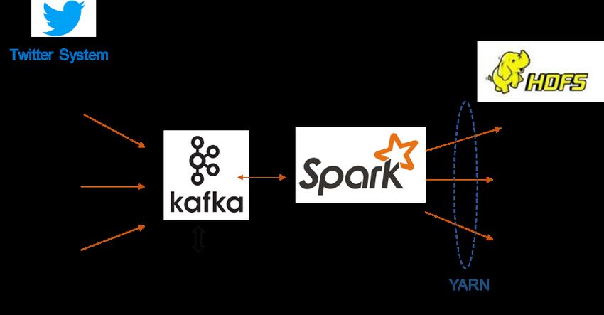
Big Data Cogn. Comput. 2021, 5, 46 2 of 30

 connectivity within itself than it does compared to the average connectivity of the graph
 as a whole, and also has appeared in various forms in several other disciplines.
 Over the last two decades, data generated by people, machine and organizations
 have been increasing rapidly. This modern data can no longer be managed and analyzed
 using the traditional technologies, leading to the birth of a new field, namely, big data.
 The field of big data analysis is associated with its ”Five Vs”, which are volume, velocity,
 variety, veracity and value. The needed technologies have been developed to tackle the
 first four of these in order to find value; among those are Apache Hadoop and Spark.
 While Hadoop with its Hadoop File Systems (HDFS) and YARN handles the distributed
 storage and resource management in the cluster, which may include thousands of ma-
 chines, Spark, running on top of YARN with its Resilient Distributed Datasets (RDD), pro-
 vides speedy parallel computing with distributed memory. Together, they can process
 petabytes of big data. The Machine Learning libraries implemented in Spark are designed
 for very simple use [6], and Spark is also well-suited to handling big graphs [5].
 Spark’s GraphX is a graph processing system. It is a layer on top of Spark that pro-
 vides a graph data structure composed of Spark RDDs. It provides an API to operate on
 those graph data structures [5]. GraphX API provides standard algorithms, such as Short-
 est Paths, Connected Components and Strongly Connected Components. The Connected
 Components algorithm is relevant for both directed and undirected graphs. For directed
 graphs, Strongly Connected Components can be used to detect vertices that have “recip-
 rocated connections”.
 Dave et al. [8] developed GraphFrames, an integrated system that lets Spark users
 combine graph algorithms, pattern matching and relational queries and optimize work
 across them. A GraphFrame is logically represented as two DataFrames: an edge Data-
 Frame and a vertex DataFrame. To make applications easy to write, GraphFrames provide
 a concise, declarative API based on the “data frame” concept. The pattern operator enables
 easy expression of pattern matching or motif finding in graphs. Because GraphFrames is
 built on top of Spark, it has the capability to process graphs having millions or even bil-
 lions of vertices and edges stored in distributed file systems (such as HDFS in Hadoop).
 As previously mentioned, communities can be uncovered from social media data
 such as tweets from Twitter. Tweets are considered as big data in a stream. Stream pro-
 cessing is a key requirement of many big data applications [6]. Based on the methodology
 for processing data streams, a data stream can be classified as either an online (live) data
 stream or as an off-line (archived) data stream [9]. An important distinction between off-
 line and online is that the online method is constrained by the detection and reaction time
 (due to the requirement of real-time applications) while the off-line is not. Depending on
 its objective (such as finding trending topics, vs. detecting communities), a stream of
 tweets can be processed either online or off-line.
 We found that unlike “fixed” communities that can be uncovered from users’ follow-
 ing/follower behaviors, temporal “informal”, communities can also be detected from
 batches of tweet streams; each batch is collected during a certain period of time (such as
 daily or weekly), thus, applying the off-line stream computation approach. For this pur-
 pose, graphs are created from users’ interaction through the reply and quote status of each
 tweet. The user IDs become the nodes, while the replies or quotes among users are trans-
 lated into edges. Intuitively, a group of people who frequently interact with each other
 during a certain short period become a community (at least during that period). Thus, the
 more frequent a group of users interact with each other, the more potential there is for a
 community to be formed among those users. In this regard, we found that the communi-
 ties formed from one period of time to another are very dynamic. The number of commu-
 nities changes from one period to another, as do the members in each community. Com-
 munities which existed in one period may disappear in the next period, whereas other
 communities may be formed. The dynamic nature of the communities is in line with the
 users’ interest towards particular tweets’ content, which varies over time.

Big Data Cogn. Comput. 2021, 5, 46 3 of 30

 In our study of the literature (Subsection 2.1), we found that most community detec-
 tion techniques are aimed at processing undirected graphs, and are based on the cluster-
 ing techniques. The proposed algorithms take the size of a cluster or a community as one
 of their inputs. For processing big data such as batches of tweets this approach poses a
 weakness, as the exact number of communities is not known in advance. Moreover, the
 number of communities that can be discovered may change from batch to batch. We also
 found that most community detection algorithms are complex and thus difficult to imple-
 ment, particularly on a distributed framework such as Spark.
 As data accumulates, data science has been becoming necessity for a variety of or-
 ganizations. When aiming to discover insights, stages in data science include: defining the
 problems to be solved by the data; its collection and exploration; its preparation the data
 (feature engineering); finding algorithms, techniques or technologies that are suitable for
 solving problems; performing data analysis; and evaluating the results. If the results are
 not satisfying, the cycle of stages is repeated. The vast majority of work that goes into
 conducting successful analyses lies in preprocessing data or generating the right features,
 as well as selecting the correct algorithms [10]. Given the objective of uncovering “tem-
 poral communities” from batches of tweets and the advantages that have been discussed
 in the previous paragraphs, Spark provides Dataframes, GraphX and GraphFrames that
 can be best utilized to process big graphs. The technique could be simple yet effective and
 scalable for processing big graphs.
 In this work, we propose a concept of temporal communities, then develop tech-
 niques that are effective for uncovering those communities from directed graphs in the
 Spark environment. The case study is of directed graphs prepared from a dataset of tweet
 batches. The criteria of the proposed technique are that it is able to (1) discover communi-
 ties without defining the number of communities, (2) handle directed big graphs (up to
 millions of vertices and/or edges); and (3) take advantages of the Dataframes, GraphX and
 GraphFrames APIs provided by Spark in order to process big data. We also propose a
 method for preparing the directed graphs that effectively supports the findings. While
 most of the communities’ detection techniques (see Section 2.1) have been developed for
 undirected graphs, we intend to contribute techniques for processing directed big graphs,
 especially using APIs provided by Spark. Although our proposed technique is based on
 the intention to analyze graphs of tweets, it will also be useful for other directed graphs
 created from other raw (big) data, such as web page clicks, messaging, forums, phone
 calls, and so on.
 In essence, the major contributions of this paper are summarized as follows:
 (1) The concept of temporal active communities suitable for social networks, where the
 communities are formed based on the measure of their interactions only (for every
 specific period of time). There are three communities defined: similar interest com-
 munities (SIC), strong-interacting communities (SC), and strong-interacting commu-
 nities with their “inner circle” neighbors (SCIC).
 (2) The algorithms to detect SIC, SC and SCIC from directed graphs in an Apache Spark
 framework using DataFrames, GraphX and GraphFrames API. As Spark provides
 data stream processing (using Spark Streaming as well as Kafka), the algorithms can
 potentially be used for analyzing the stream via the off-line computation approach
 for processing batches of data stream.
 (3) The use of motif finding in GraphFrames to discover temporal active communities.
 When the interaction patterns are known in advance, motif finding can be employed
 to find strongly connected component subgraphs. This process can be very efficient
 when the patterns are simple.
 This paper is organized as follows: Section 2 discusses related work on community
 detection techniques as well as work that has been done in analyzing Twitter data and the
 big data technologies employed in this research, which are Spark, GraphX, and
 GraphFrames. Section 3 excerpts the results of the experiment comparing Strongly

Big Data Cogn. Comput. 2021, 5, 46 4 of 30

 Connected Component algorithm and motif findings on Spark. Section 4 presents our pro-
 posed techniques. Section 5 discusses the experiments using public and Twitter data. In
 Section 5, we present our conclusions and further works.

 2. Literature Review
 2.1. Related Works
 Formidably sized networks are becoming more and more common, such that many
 network sizes are expected to challenge the storage capability of a single physical com-
 puter. Fung [11] handles big networks with two approaches: first, he adopts big data tech-
 nology and distributed computing as storage and processing, respectively. Second, he de-
 velops discrete mathematics in InfoMap for the distributed computing framework and
 then further develops the mathematics for a greedy algorithm, called InfoFlow, for detect-
 ing communities from undirected big graphs. InfoMap and InfoFlow are implemented on
 Apache Spark using the Scala language. The InfoFlow performance is evaluated using big
 graphs of 50,515 to 5,154,859 vertices and the results show that the runtime complexity of
 InfoFlow had logarithmic runtime complexity, while retaining accuracy in the resulted
 community
 The existing community detection algorithms principally propose iterative solutions
 of high polynomial order that repetitively require exhaustive analysis. These methods can
 undoubtedly be considered, resource-wise, to be overdemanding, unscalable, and inap-
 plicable in big data graphs such as today’s social networks. To address these issues, Ma-
 kris and Pispirigos [3] proposed a novel, near-linear, and scalable community prediction
 methodology. Using a distributed, stacking-based model, the underlined community hi-
 erarchy of any given social network is efficiently extracted in spite of its size and density.
 Their proposed method consists of three stages: first, subgraph extraction (the bootstrap
 resampling method is adopted and multiple BFS crawlers are randomly triggered to ex-
 tract subgraphs of a predefined size; the maximum number of BFS crawlers, which are
 concurrently executed, is practically determined by the level of parallelism of the execu-
 tion system); second, feature enrichment (each individual edge is properly enriched with
 features that include its network topology information up to a predefined depth of a value
 k; The value of k is an essential parameter that seriously affects the community prediction’s
 performance); third, a stacking ensemble learner is employed to detect communities (the
 independently trained, heterogeneous base learners are aptly combined by training a final
 model relying on the individual base learners’ predictions; it is built on top of a distributed
 bagging ensemble of L2 regularized, binary logistic regression classifiers, and a distrib-
 uted gradient boosted trees ensemble model, also known as distributed GBT boosting en-
 semble model). To evaluate the methods, the experiments were conducted on Spark clus-
 ter with eight nodes using seven undirected and directed graphs (available at
 https://snap.stanford.edu/data/, accessed on 19 March 2021) having 1858 to 154,908 verti-
 ces. For evaluating the communities, the metrics measured are accuracy, recall, precision,
 specificity and F1-score. The metric values show that the models have detected the com-
 munities accordingly. The execution time of stacking ensemble methods executed in par-
 allel on the Spark cluster beats that of the Louvain and Girwan–Newman methods that
 run on single node.
 Bae et al. [1] developed a parallel algorithm for graph clustering called RelaxMap that
 parallelizes the optimization of flow-compression for community detection. It employs a
 prioritization strategy that avoids handling vertices that do not significantly improve the
 algorithm. The core algorithm works in two phases. In Phase 1, the visit probability (rank)
 of each vertex is computed in terms of the network flow. In Phase 2, tthe space of possible
 modularizations is greedily searched. In the search procedure for the best new module of
 a vertex v, the algorithm calculates the total in-flow and total out-flow between the vertex
 v and its neighbor modules (i.e., the set of modules to which any of its neighbors belong).

Big Data Cogn. Comput. 2021, 5, 46 5 of 30

 The algorithm stops when the change in the minimum description length (MDL) score in
 each iteration is less than a minimum quality improvement threshold, Lprev − L < τ.
 Bhatt et al. [12] proposed a community detection and characterization algorithm that
 incorporates the contextual information of node attributes described by multiple domain-
 specific hierarchical concept graphs. The core problem is to find the context that can best
 summarize the nodes in communities, while also discovering communities aligned with
 the context summarizing communities. The proposed algorithm iteratively optimizes two
 tasks, (i) optimal community label assignment while keeping the community context un-
 changed, and (ii) optimal community context assignment while keeping the community
 labels constant.
 Most of the existing community detection methods have been proposed based exclu-
 sively on social connections. The emergence of geo-social networks (GeoSNs) motivates
 the integration of location information in community detection. In this context, a commu-
 nity contains a group of users that are tightly connected socially and are situated in the
 same geographic area. Yao, Papadias and Bakiras [4] have proposed a model called Den-
 sity-based Geo-Community Detection (DGCD) in geo-social networks. This model ex-
 tends the density-based clustering paradigm to consider both the spatial and social rela-
 tionships between users. The results of the experiment show that the proposed model
 produces geo-social communities with strong social and spatial cohesiveness, which can-
 not be captured by existing graph or spatial clustering methods.
 In [13], Jia et al. proposed CommunityGAN, a community detection framework that
 jointly solves overlapping community detection and graph representation learning. Com-
 munityGAN aims to learn network embeddings like AGM (Affiliation Graph Model)
 through a specifically designed GAN. AGM is a framework which can model densely
 overlapping community structures. It assigns each vertex-community pair a nonnegative
 factor which represents the degree of membership of the vertex to the community. Thus,
 the strengths of membership from a vertex to all communities compose the representation
 vector of it. The algorithm of CommunityGAN takes as inputs the number of communities
 c, size of discriminating samples m, and size of generating samples n.
 Roghani, Bouyer and Nourani [14] proposed a Spark-based parallel label diffusion
 and label selection-based (PLDLS) community detection algorithm using GraphX, which
 is an improved version of LPA, by putting aside randomness parameter tuning. PLDLS
 introduces NI, which is the importance measure of a node, used to find core nodes that
 initially form communities. For every node, NI(i) is locally computed using the following
 equation:
 ( ) = _ ( ) × deg ( )2 (1)
 
 where ( ) = and deg(i) is the degree measure of ith node.
 ∑ ∈ , 
 In essence, PLDLS steps are as follows: Using GraphX, the input dataset is repre-
 sented as an RDD containing pairs of vertex and edge collections, G(V,E). NI(i) is com-
 puted in parallel using Equation 1. Nodes having NI(i) ≥ Average (NI of all nodes) are
 selected. The modes of these selected nodes are computed. The communities are initial-
 ized with the member of core nodes with NI(i) ≥ mode of NI. The communities are then
 expanded by diffusing with their neighbors, to include first and second level nodes. First-
 level nodes are groups of neighbors (FLIN) that form a triangle with a core node and its
 most important neighbor; all of them at once get the same label. Second-level nodes are
 the neighbor nodes of FLIN that satisfy NI(FLIN) ≥ NI(i) and have Jaccard similarity higher
 than 0.5. Through iterative computation, the rest of the nodes (the unlabeled ones) are
 visited and labeled with their community ID. Using Pregel functions, the labels are im-
 proved, then the communities are merged in parallel (to integrate communities that are
 likely to be merged) in order to obtain more dense and accurate communities.
 In real world networks, such as interpersonal relationship in human society and ac-
 ademic collaboration networks, communities tend to overlap. Thus, finding the overlap-
 ping community structure in complex networks is needed. As reported in [15],

Big Data Cogn. Comput. 2021, 5, 46 6 of 30

 LinkSHRINK is an overlapping community detection method that combines density-
 based clustering with modularity optimization in a link graph. It finds overlapping com-
 munities by merging reductant nodes with parameter ω. It avoids the problem of exces-
 sive overlapping and reveals the overlapping community structure with different overlap
 degrees by using parameter ω. To find overlapping communities in large-scale networks,
 Zhang et al. [15] parallelized LinkSHRINK on Spark using GraphX (named as
 PLinkSHRINK) and Hadoop using Map-Reduce jobs (named as MLinkSHRINK).
 Through a series of experiments using synthetic and real networks, it is reported that: (1)
 while LinkSHRINK cannot handle very large graphs, PLinkSHRINK and MLinkSHRINK
 can find communities in large networks with millions of edges efficiently without losing
 significant accuracy; (2) on Spark, the running time of PLinkSHRINK correlates with the
 executer cores, or performance improves with an increasing number of cores; and (3)
 PLinkSHRINK runs faster on large networks than MLinkSHRINK and LinkSHRINK.
 DENCAST [16] is a parallel clustering algorithm for Spark. It is based on a well-
 known density-based clustering algorithm, DBSCAN, which is able to identify arbitrarily
 shaped clusters. DBSCAN works iteratively and needs two parameters, which are eps
 (maximum distance of objects) and minPts (minimum points). DBSCAN starts with an
 arbitrary object o and, if this is a core object, it retrieves all the objects which are density-
 reachable from the core by using eps and minPts, and returns a cluster. The algorithm
 then proceeds with the next unclustered object until all objects are visited. Thus, DBSCAN
 works with graphs that represent the objects and their neighbors. Using GraphX on Spark,
 DENCAST identifies the reachable nodes of all the core objects simultaneously. This is
 performed by propagating the cluster assignment of all the core objects to their neighbors
 until the cluster assignment appears stable enough. Based on the evaluation experiments
 on a Spark cluster, it was concluded that DENCAST is able to handle large-scale and high-
 dimensional data. The model has high accuracy. It also significantly outperforms the dis-
 tributed version of K-means in Apache Spark in terms of running times.
 In [17], Krishna and Sharma discuss the review results of five parallel community
 detection algorithms, as follows: (1) the distributed memory-based parallel algorithm
 based on modularity maximization proposed by Louvain and implemented on an MPI-
 based HPC cluster; (2) Picaso, a parallel community detection model based on approxi-
 mate optimization. It is based on two approaches: a computing “mountain” (of vertices)
 based on approximate optimization and modularity, and the Landslide algorithm, which
 is iterative and implemented using GraphX on Spark; (3) FPMQA, a parallel modularity
 optimization algorithm that uses the modularity technique to identify communities in the
 social networks. The networks are initialized with people connected based on their com-
 ments on similar topic of interests, namely similar view network (SVN). The FPMQA al-
 gorithm is executed in parallel to process this SVN (there will be a group of nodes con-
 nected in this SVN due to common interest). Based on gain modularity measures, SVNs
 may be merged. The modularity computation is done in parallel; (4) PLPAC, a label prop-
 agation-based parallel community detection algorithm with nodes confidence. In label
 propagation algorithm (LPA), each node label (denoting its community ID) is updated
 based on the labels with the highest modularity among their neighbors. The proposed
 parallel algorithm is implemented using MapReduce; (5) an algorithm for detecting dis-
 jointed communities on large-scale networks, which is based on the Louvain algorithm
 and implemented for parallel shared memory. All of the algorithms discussed in [17] work
 with undirected graphs, or do not consider direction (of the edges between nodes) as im-
 portant for finding communities.
 Atastina et al. [7] discusses how to process communication transaction data to find
 the communities and track the evolution of the communities over time. The Facetnet al-
 gorithm, which is based on clustering vertices, is applied to undirected graphs to mine the
 communities.

Big Data Cogn. Comput. 2021, 5, 46 7 of 30

 Twitter messages or tweets, which originate from all over the world using many lan-
 guages, have also attracted researchers. Three examples of recent work results are ex-
 cerpted below.
 In a case study using Twitter data, Sadri et al. [18] analyzed the characteristics and
 growth of online social interaction networks, examining the network properties and de-
 riving important insights based on the theories of network science literature. The data is
 specific to the Purdue University community. They collected tweets (between 16 April
 2016 and 16 May 2016) using a specific keyword ‘purdue’ and captured 56,159 tweets. Of
 these tweets, 19,532 did not include any user mentions, while the rest of the tweets in-
 cluded at least one user mention in each tweet. The dataset contains 34,363 unique users
 and 38,442 unique undirected links (39,709 links if direction is considered). The graphs,
 which are created from users and their mentions, are analyzed as both undirected and
 directed graphs, using visualization, vertex degree (including in-out degree), graph ra-
 dius, connected component and clustering. Key insights found were: (i) the graph indi-
 cated that with some vertices being highly active, there are connected components and
 hubs; (ii) network elements and average user degree grow linearly each day, but network
 densities tend to become zero, and the largest connected components exhibit higher con-
 nectivity when compared to the whole graph; (iii) network radius and diameter become
 stable over time, which suggests a small-world property.
 All of the above community detection techniques do not discuss the importance of
 edge direction. The directed graphs discussed in [18] are only used to compute in-out
 degree.

 2.2. Spark, GraphX and GraphFrames
 2.2.1. Apache Spark
 Apache Spark is a data processing framework that is fast and scalable for processing
 big data, employing non-iterative as well as iterative algorithms. It is written in Scala and
 runs in Java Virtual Machine (JVM). For processing big data, Spark is more often used in
 tandem with a distributed storage system (such as Hadoop Distributed File System,
 HDFS) and a cluster manager, such as Apache Hadoop YARN [6,19,20]. HDFS is a distrib-
 uted file system designed to reliably store very large files across machines in a large clus-
 ter. Each HDFS file is stored as a sequence of blocks; these blocks are replicated for fault
 tolerance. Apache Hadoop YARN (Yet Another Resource Negotiator) provides the re-
 source management and job scheduling for Hadoop clusters, consisting of master and
 data (slave/worker) nodes [21,22]. As YARN is able to manage clusters each with thou-
 sands of machines, it supports Spark scalability for processing big data. When run on top
 of YARN, a physical Spark cluster that consists of driver and worker machines may have
 thousands of workers that can run parallel tasks on the workers.
 Resilient Distributed Datasets. Spark is built around a data abstraction called Resili-
 ent Distributed Datasets (RDD). An RDD is an immutable distributed collection of objects
 and is commonly split into multiple partitions [19,23]. Those partitions are stored across
 worker nodes’ memory if Spark is run on YARN or another resource manager. Each par-
 tition of an RDD can be processed by one task or more that run parallel across the core
 machines, which speeds up overall computation. Once created, RDDs offer two types of
 operations, transformations and actions. Actions are functions that return values that are
 not RDDs, whereas transformations return other forms of RDD. Each Spark application
 must contain at least one action (such as collect, count, take and saveAsTextFile), since
 actions either bring information back to the driver or write the data to stable storage.
 Transformations (such as sort, reduce, group and filter) construct new RDDs from the old
 ones. Transformations and actions are different because of the way Spark computes RDDs.
 Operations on RDDs are queued up in a lazy fashion and then executed all at once only
 when needed, that is, when an action is called. At this time, Spark optimizes those opera-
 tions and also plans data shuffles (which involve expensive communication, serialization,

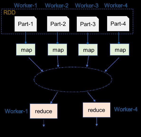
Big Data Cogn. Comput. 2021, 5, 46 8 of 30

 and disk I/O) and generates an execution graph, the Directed Acyclic Graph (DAG), de-
 tailing a series of execution plans; it then executes these plans [5]. Spark can keep an RDD
 loaded in-memory on the executor nodes throughout the life of a Spark application for
 faster access in repeated computations [21].
 Spark Application. A Spark application corresponds to a set of Spark jobs defined by
 one SparkContext in the driver program [4]. A Spark application begins when a Spark-
 Context is started, which causes a driver and a series of executors be started on the worker
 nodes of the cluster. Each executor corresponds to a JVM. The SparkContext determines
 how many resources are allotted to each executor. When a Spark job is launched, each
 executor has slots for running the tasks needed to compute an RDD. Physically, each task
 runs on a machine core, and one task may process one or more RDD partition (when an
 RDD is created by loading a HDFS file, the default is: Spark creates an RDD partition for
 each HDFS block, and stores this partition in the memory of the machine that has the
 block). One Spark cluster can run several Spark applications concurrently. The applica-
 tions are scheduled by the cluster manager and correspond to one SparkContext.
 A Spark application can run multiple concurrent jobs, whereas a job corresponds to
 an RDD action that is called (see Figure 1). That is, when an RDD action is called, the Spark
 scheduler builds a DAG and launches a job. Each job consists of stages. One stage corre-
 sponds to one wide-transformation, which occurs when a reducer function that triggers
 shuffling data (stored as RDD partitions) across the network is called (see Figure 2). Each
 stage consists of tasks, which are run in parallel, and each task executes the same instruc-
 tion on an executor [19,23]. The number of tasks per stage depends on the number of RDD
 partitions and the outputs of the computations.

 Spark Spark Context (Spark Session Object)
 Application

 RDD Actions (e.g.,
 Job Job saveAsTextFile, collect)

 Wide transformation (e.g.,
 Stage Stage Stage
 reduceByKey, sort)

 Computation to evaluate
 Task Task Task Task Task one RDD partition (narrow
 transformations)

 Figure 1. The Spark application tree [23].

 Examples of transformations that cause shuffling include groupByKey, reduce-
 ByKey, aggregateByKey, sortByKey, and join. Several narrow transformations (such as
 map, filter, mapPartitions and sample) are grouped into one stage. As shuffling is known
 as an expensive operation and can degrade computation, it is necessary to design Spark
 applications that involve minimum number of shuffles or stages to achieve better perfor-
 mance.

Big Data Cogn. Comput. 2021, 5, 46 9 of 30

 Figure 2. Illustration of shuffling for a stage on a Spark cluster with four workers: each worker stores
 one RDD partition and runs a map task, then two reducer tasks on two workers process data from
 map tasks.

 2.2.2. GraphX and GraphFrames
 GraphX is an embedded graph processing framework built on top of Apache Spark.
 It implements a notion called the property graph, whereby both vertices and edges can
 have arbitrary sets of attributes associated with them. GraphX recasts graph-specific op-
 timizations as distributed join optimizations and materialized view maintenance [24]. Us-
 ers can simply use GraphX’s API to operate on those graph data structures [5]. This pro-
 vides a powerful low-level interface. However, like RDDs it is not easy to use or optimize.
 However, GraphX remains a core part of Spark for graph processing [6].
 Distributed Graph Representation [24]: GraphX represents graphs internally as a pair
 of vertex and edge collections built on the RDD abstraction. These collections introduce
 indexing and graph-specific partitioning as a layer on top of RDDs. The vertex collection
 is hash-partitioned by the vertex IDs. To support frequent joins across vertex collections,
 vertices are stored in a local hash index within each partition. The edge collection is hori-
 zontally partitioned. GraphX enables vertex-cut partitioning. By default, edges are as-
 signed to partitions based on the partitioning of the input collection (e.g., the HDFS
 blocks). A key stage in graph computation is constructing and maintaining the triplets
 view, which consists of a three-way join between the source and destination vertex prop-
 erties and the edge properties. The techniques used include Vertex Mirroring, Multicast
 Join, Partial Materialization, and Incremental View Maintenance.
 GraphX API provides an implemented standard algorithm, such as PageRank, Con-
 nected Components and Strongly Connected Components (SCC). While the Connected
 Components algorithm is relevant for both directed and undirected graphs, Strongly Con-
 nected Components is for directed graphs only, and can be used to detect vertices that
 have “reciprocated connections”. A few of the graph algorithms, such as SCC, are imple-
 mented using Pregel.
 The Pregel algorithm that computes SCCs from a directed graph G = (V,E) is ex-
 cerpted as follows.
 Let SCC(v) be the SCC that contains v, and let Out(v) (and In(v)) be the set of vertices
 that can be reached from v (and that can reach v) in G, then SCC(v) = Out(v)∩ In(v). Out(v)
 and In(v) are computed by forward/backward breadth-first search (BFS) from a source v
 that is randomly picked from G. This process then repeats on G[Out(v)- SCC(v)], G[In(v)-
 SCC(v)] and G[V- (Out(v)ՍIn(v)-SCC(v))], where G[X] denotes the subgraph of G induced
 by vertex set X. The correctness is guaranteed by the property that any remaining SCC
 must be in one of these subgraphs.

Big Data Cogn. Comput. 2021, 5, 46 10 of 30

 Yan et al. [25] designed two Pregel algorithms based on label propagation. The first
 propagates the smallest vertex (ID) that every vertex has seen so far (namely, the miLabel
 algorithm), while the second propagates multiple source vertices to speed up SCC com-
 putation (namely, multi-Label algorithm). miLabel algorithm requires a graph decompo-
 sition, which allows the algorithm to run multiple rounds of label propagation.
 Graph Decomposition: given a partition V, denoted by V1, V2,…, Vl, G is decomposed
 into G[V1], G[V2],…, G[Vl] in two supersets (here, each vertex v contains a label i indicating
 v ε Vi): (i) each vertex notifies all its in-neighbors and out-neighbors about its label i; (ii)
 each vertex checks the incoming messages, removes the edges from/to the vertices having
 labels different from its own label, and votes to halt.
 MinLabel Algorithm: the min-label algorithm repeats the following operations: (i)
 forward min-label propagation; (ii) backward min-label propagation; (iii) an aggregator
 collects label pairs (i, j), and assigns a unique ID to each V(i,j); graph decomposition is then
 performed to remove edges crossing different G[VID]; finally, each vertex v is labeled with
 (i; i) to indicate that its SCC is found. In each step, only unmarked vertices are active, and
 thus vertices do not participate in later rounds once their SCC is determined. Each round
 of the algorithm refines the vertex partition of the previous round. The algorithm termi-
 nates once all vertices are marked.
 GraphX Weaknesses: GraphX limitations stem from the limitations of Spark. GraphX
 is limited by the immutability of RDDs, which is an issue for large graphs [5]. In some
 cases, it also suffers from a number of significant performance problems [21].
 GraphFrames extends GraphX to provide a DataFrame API and support for Spark’s
 different language bindings so that users of Python can take advantage of the scalability
 of the tool [6]. So far, it is a better alternative to GraphX [21]. GraphFrames is an integrated
 system that lets Spark users combine graph algorithms, pattern matching and relational
 queries, and optimizes work across them. A GraphFrame is logically represented as two
 DataFrames: an edge DataFrame and a vertex DataFrame [8].
 In Spark, DataFrames are distributed as table-like collections with well-defined rows
 and columns [6]. These consist of a series of records that are of type Row, and a number
 of columns that represent a computation expression that can be performed on each indi-
 vidual record in the Dataset. Schemas define the name as well as the type of data in each
 column. Spark manipulates Row objects using column expressions in order to produce
 usable values. Filtering and applying aggregate functions (count, sum, average, etc.) to
 group records are among these useful expressions. With its lazy computation (see Section
 2.2.1), whenever Spark receives a series of expressions for manipulating DataFrames that
 need to return values, it analyzes those expressions, prepares a logical optimized execu-
 tion plan, creates a physical plan, then executes the plan by coordinating with the resource
 manager (such as YARN) to generate parallel tasks among the workers in the Spark clus-
 ter.
 GraphFrames generalizes the ideas in previous graph-on-RDBMS systems, by letting
 the system materialize multiple views of the graph and executing both iterative algo-
 rithms and pattern matching using joins [8]. It provides a pattern operator that enables
 easy expression of pattern matching in graphs. Typical graph patterns consist of two
 nodes connected by a directed edge relationship, which is represented in the format ()-[]-
 >(). The graph patterns as the input of the pattern operator are usually called network
 motifs, which are sub-graphs that repeat themselves in the graph that is analyzed. The
 pattern operator is a simple and intuitive way to specify pattern matching. Under the
 hood, it is implemented using the join and filter operators available on a GraphFrame.
 Because GraphFrames builds on top of Spark, this brings three benefits: (i)
 GraphFrames can load data from the volumes saved data in many formats supported by
 Spark (GraphFrames has the capability of processing graphs having millions or even bil-
 lions of vertices and edges); (ii) GraphFrames can use a growing list of machine learning
 algorithms in MLlib; and (iii) GraphFrames can call the Spark DataFrame API.

Big Data Cogn. Comput. 2021, 5, 46 11 of 30

 One case of using GraphFrames is discussed in [26], where an efficient method of
 processing SPARQL queries over GraphFrames was proposed. The queries were applied
 to graph data in the form of a Resource Description Framework (RDF) that was used to
 model information in the form of triples , where each edge can
 be stored as a triple. They created queries based on two types of SPARQL queries, chain
 queries and star-join queries. The experiments were performed using the dataset pro-
 duced by the Lehigh University benchmark (LUBM) data generator, which is a synthetic
 OWL (Web Ontology Language) dataset for a university. Overall, the proposed approach
 works well for large datasets.

 3. Comparing SCC Algorithm and Motif Finding on Spark
 As presented in Section 2.2.2, GraphFrames provides graph pattern matching (motif
 finding). We found that SCC subgraphs used to uncover active communities from di-
 rected graphs can be detected using GraphX SCC algorithm as well motif finding. In this
 section, we present our experimental results of SCC algorithm and motif finding perfor-
 mance.
 As discussed in Section 2.2.1, data shuffling across a Spark cluster is expensive. When
 an algorithm for processing big data is run, Spark generates a stage whenever it encoun-
 ters a wide transformation function, a computation that requires shuffling among RDD
 partitions across the network. Using the Spark web UI, we can observe and learn several
 kinds of computation statistics, DAG, execution plan and other related information re-
 garding the applications being run. The DAG, execution plan, jobs, stages and parallel
 tasks can be used to measure the complexity of the program or algorithm that is run.
 We created seven synthetic small graph datasets (g1, g2, … , g7), each consisting of
 vertex and edge dataframes. Each of the six datasets has an SCC subgraph that is shown
 in Figure 3, while one dataset (g7) contains all of the SCC subgraphs.

 Figure 3. Six SCC subgraphs to be detected from graph dataset: (a) g1, (b) g2, (c) g3, (d) g4, (e) g5,
 (f) g6.

 As the synthetic datasets are small, we performed these experiments on a Spark clus-
 ter with a single machine with i7-3770 CPU, four cores and 16 Gb memory. The cluster
 ran Apache Spark 2.4.5, Java 1.8.0_40, and Scala 2.11.12. The following steps were per-
 formed for each graph dataset:

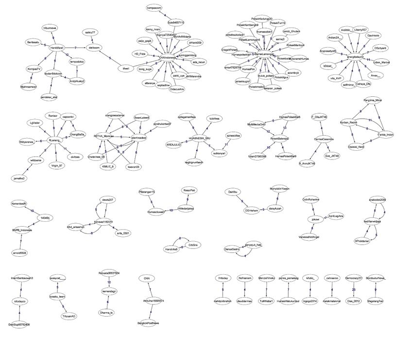
Big Data Cogn. Comput. 2021, 5, 46 12 of 30

 (1) An instance of GraphFrame for each graph dataset was created;
 (2) SCC algorithm was used to detect SCCs from the graph instance;
 (3) A set of patterns was searched from the graph instance. The pattern set searched on
 g1 was “(a)-[e1]->(b); (b)-[e2]->(a)”, g2 was “(a)-[e1]->(b); (b)-[e2]->(c); (c)-[e3]->(a)”,
 g3 was “(a)-[e1]->(b); (b)-[e2]->(c); (c)-[e3]->(d); (d)-[e4]->(a)”, g4 was “(a)-[e1]->(b);
 (b)-[e2]->(c); (c)-[e3]->(b); (b)-[e4]->(a)”, g5 was “(a)-[e1]->(b); (b)-[e2]->(c); (c)-[e3]-
 >(d); (d)-[e4]->(e); (e)-[e5]->(a)”, and g6 was “(a)-[e1]->(b); (b)-[e2]->(c); (c)-[e3]->(b);
 (b)-[e4]->(a);(c)-[e5]->(d); (d)-[e6]->(c)”. For g7, all of the patterns were combined.
 Then the execution time as well as the information on the Spark web UI were ob-
 served on each run and recorded.
 The Scala codes executed in these experiments are attached in Appendix A.
 As discussed in Section 2.2.2, motif findings were executed using the join and filter
 operators. For instance, below is the optimized logical plan of query (a), g1.find(“(a)-[e1]-
 >(b); (b)-[e2]->(a)”) generated by Spark:
 1 +- Project [cast(a#34 as string) AS a#83, cast(e1#32 as string)
 AS e1#84, cast(b#36 as string) AS b#85, cast(e2#57 as string)
 AS e2#86]
 2 +- Join Inner, ((e2#57.src = b#36.id) && (e2#57.dst = a#34.id))
 3 :- Join Inner, (e1#32.dst = b#36.id)
 4 : :- Join Inner, (e1#32.src = a#34.id)
 5 : : :- Project [named_struct(src, src#10, dst, dst#11, weight, weight#12) AS e1#32]
 6 : : : +- Relation[src#10,dst#11,weight#12] csv
 7 : : +- Project [named_struct(id, id#26) AS a#34]
 8 : : +- Relation[id#26] csv
 9 : +- Project [named_struct(id, id#26) AS b#36]
 10 : +- Relation[id#26] csv
 11 +- Project [named_struct(src, src#10, dst, dst#11, weight, weight#12) AS e2#57]
 12 +- Relation[src#10,dst#11,weight#12] csv
 In the plan above, the inner join (between vertex and edge dataframes) is performed
 three times, to resolve part of the query “(a)-[e1]” (line 4), “(a)-[e1]->(b)” (line 3) and “(b)-
 [e2]->(a)” (line 2). As discussed in Section 2.2.1, a Spark job is created when an application
 calls an RDD action. Here, a job is created each time a project (filter) operation is applied
 to the result of the join (line 5, 7, 9, and 11). Thus, there are four jobs. The overall DAG is
 shown on Figure 4. In the physical execution plan, the inner join is implemented by Broad-
 castExchange then BroadcastHashJoin. Broadcasting records stored in the RDD partitions
 causes data shuffling (such as in wide transformation) that produces one stage. Hence,
 there are four stages (one job only having one stage). Other queries of motif findings are
 executed using join and filter, analogous to (a); the number of jobs and stages is presented
 on Table 1.

Big Data Cogn. Comput. 2021, 5, 46 13 of 30

 Figure 4. The DAG of motif finding of SCC from g1, Cyclic_2.

 Unlike motif findings, which implement queries where the execution plan is availa-
 ble for observation, when running the SCC algorithm (as with other algorithms designed
 based on RDD) we can only observe the execution process through its jobs, stages, DAG
 and tasks. As can be observed, when the SCC algorithm is run it requires many jobs and
 stages (see Table 1). For instance, when processing g1, Spark generates 29 jobs. As an ex-
 ample, the DAG of its sixth job (with Id 9) with three stages is provided in Appendix A,
 Figure A1: Stage 14 performs mapping at GraphFrame, Stage 13 performs mapPartition-
 ing at VertexRDD, and Stage 15 folding at VertexRDDImpl. From the number of jobs,
 stages and DAG, we can learn that the implementation of the iterative SCC algorithm on
 Spark (see Section 2.2.2) is complex and requires lots of machine and network resources.

 Table 1. Comparison of Spark jobs and stages.

 Motif Finding SCC Algorithm
 Case Graph
 #Jobs #Stages #Jobs #Stages
 (a) g1 4 4 29 75
 (b) g2 6 6 28 75
 (c) g3 8 8 30 83
 (d) g4 7 7 32 80
 (e) g5 10 10 38 105
 (f) g6 10 10 37 98
 (g) g7 45 45 41 114

 In line with the number of jobs and stages (Table 1), the execution time of each motif
 finding is also smaller compared to the SCC algorithm (see Figure 5).
 It is known that hash-join time complexity is O(n+m), where n + m denotes the total
 records in two tables being joined. On a system with p cores, the expected complexity of

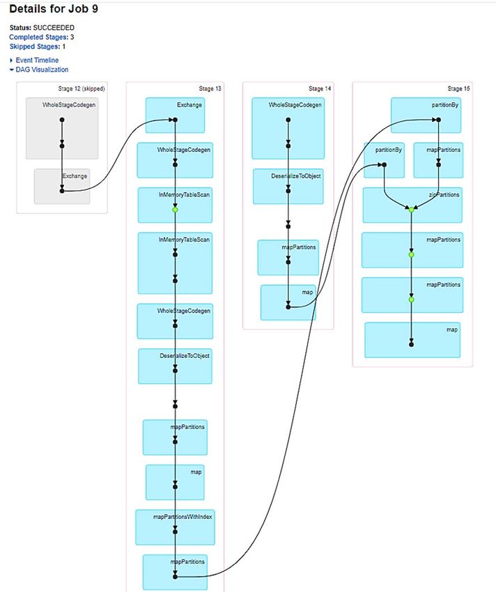
Big Data Cogn. Comput. 2021, 5, 46 14 of 30

 the parallel version of no partitioning hash join is O((n + m)/p) [27]. Although this com-
 plexity it not specifically applied for hash join in Spark, the motif finding execution time
 seems to be in line with O((n + m)/p).
 The time complexity of parallel SCC algorithm for Spark is not discussed in [8] and
 [24]. To the best of our knowledge, it is not discussed in any other literature either. How-
 ever, by comparing the stages of SCC versus motif finding presented in Table 1, it can be
 learned that the SCC computation is far more complex than the motif finding.

 Figure 5. Execution time of motif finding vs. SCC algorithm.

 Findings of these experiments: when there are not many patterns of SCC subgraphs
 in a directed graph, motif finding runs faster and uses less network resources compared
 to the SCC algorithm. Hence, this can be used as an optional technique in finding active
 communities from directed graphs.

 4. Proposed Techniques
 A streaming computational model is one of the widely used models for processing
 and analyzing massive data [9]. Based on the methodology for processing data streams, a
 data stream can be classified as an online (live stream) data stream or an off-line (ar-
 chived) data stream. Online data streams (such as those of stock tickers, network meas-
 urements, and sensor data) need to be processed online because of their high speed. An
 Off-line stream is a sequence of updates to warehouses or backup devices, where the que-
 ries over the off-line stream can be processed offline. The online method is constrained by
 the detection and reaction times due to the requirement of real-time applications, while
 the off-line is free from this requirement. Depending on its objective (such as finding
 trending topics vs. detecting communities), a stream of tweets can be processed either
 online or off-line. We proposed techniques that can be used to analyze off-line as well as
 near-real-time batches of data stream to uncover temporal active communities using the
 SCC algorithm and motif finding in Spark.

 4.1. Active Communities Definition
 Based on our observation of Twitter users’ posts, we learned that during certain pe-
 riods of time (such as weekly) lots of users either send tweets or respond to other users’
 tweets in ways that show patterns. Only tweets that draw other users’ interest were re-
 sponded to with retweet, reply or quote tweets. Thus, based on their interests that lead to
 frequent responses, Twitter users may form temporal active communities without intent.
 To form graphs that can be used to uncover these communities, the Twitter users are de-
 fined as vertices, while their interactions (reply and quote) become the edges. The number
 of interactions can be included as an edge attribute (such as weight), which then may be
 used to select the frequent vertices (vertices who communicate to each other frequently)
 by applying a threshold value.
 For a certain (relatively short) period of time, we define three types of active commu-
 nities (see Figure 6):

Big Data Cogn. Comput. 2021, 5, 46 15 of 30

 (1) Similar interest communities (SIC): A group of people responding to the same event.
 Real world examples: (a) Twitter users who frequently retweet or reply or quote a
 user’s tweets, which means that those users have the same interest toward the tweet
 content; (b) forum users who frequently give comments or reply to posts/threads
 posted by certain user/users, which means those users have the same interest in dis-
 cussion subjects.
 (2) Strong-interacting communities (SC): A group of people who interact with each other
 frequently in a period of time. Real world example: a group of people who re-
 ply/call/email/tweet/message each other.
 (3) Strong-interacting communities with their “inner circle” neighbors (SCIC): The ex-
 tension of SC, where SC members become the core of the communities, added by the
 “external” people who are frequently directly contacted by the core members, as well
 as “external” people who directly contact the core members. Real world example: as
 in the aforementioned SC, now also including the surrounding people who actively
 communicate with them.

 Figure 6. Illustration of active communities formed from a weighted-directed graph with threshold
 of edge weight = 4.

 4.2. Proposed Algorithms
 Based on the previous definition, we propose three techniques to process weighted
 directed graphs, G. G = (V, E) where V = vertices, E = edges. E must have one or more
 attributes, including its weight. V may have one attribute or more, thus E(Id, at1, at2,…),
 where Id is the Id of the vertex, followed by its attributes. E(srcId, dstId, a1, a2,…,w), where
 srcId = Id of the source vertex, dstId = Id of the target vertex, ai = i-th attribute, w = weight
 of edges, denoting the count of srcId interacts to dstId.
 (a) Detecting SIC from directed graphs
 The proposed algorithm (Algorithm 1) is simple, in that it is only based on dataframe
 queries.

 Algorithm 1: DetectSIC
 Descriptions: Detecting SIC from a directed graph using GraphFrame
 Input: Directed graph G, thWC1 = threshold of w; thIndeg = threshold of vertices
 in-degree
 Output: Communities stored in map structure, comSIC = map(CenterId, list of
 member Ids); a vertex can be member of more than one community.
 Steps:
 (1) Graph preparation: (a) filteredE = E in G with w > thWC1 //Only edges having
 w > thWC1 is used to construct the graph; (b) GFil = (V, filteredE)
 (2) Compute inDeg for every vertex in GFil, store into dataframe, inD(Id, inDegree)
 (3) selInD (IdF, inDegree) = inD where inDeg > thIndeg

Big Data Cogn. Comput. 2021, 5, 46 16 of 30

 (4) Find communities: (a) dfCom = (GFil where its nodes having Id = selInD.IdF) inner
 join with E on Id = dstId, order by Id; (b) Collect partitions of dfCom from every worker
 (coalesce) then iterate on each record: read Id and srcId column, map the pair value of
 (Id, srcId) into comSIC

 (b) Detecting SC using motif finding

 In this proposed algorithm (Algorithm 2), the data preparation is performed for re-
 ducing the number of vertices in the graphs. Only vertices passing the filter with a thresh-
 old of degree that will be further processed. In this algorithm, strongly connected sub-
 graphs, which are further processed into communities, are detected using motif findings
 described in Section 2.2 and Section 3.

 Algorithm 2: DetectSC-with-MotifFinding
 Descriptions: Detecting SC using motif finding
 Input: Directed graph G; thWC1 = threshold of w ; thDeg = threshold of vertices degree;
 motifs = {motif1, motif2, . . . , motifn} where motif1 = 1st pattern of SC, motif2 = 2nd pattern of SC,
 motifn = the nth pattern of SC
 Output: Communities stored in map structure, comSCMotif = map(member_Ids: String,
 member_count: Int) where member_Ids contains list of Id. A vertex can be member of more
 than one community.
 Steps:
 (1) Graph preparation: (a) filteredE = E in G with w > thWC1; (b) GFil = (V, filteredE)
 (2) Compute degrees for every vertex in GFil, store into a dataframe, deg(Id, degree)
 (3) selDeg (IdF, degree) = deg where degree > thDeg
 (4) Gsel = subgraph of GFil where its nodes having Id = selInD.IdF
 (5) For each motifi in motifs, execute Gsel.find(motifi), store the results in dfMi, filter rec-
 ords in dfMi to discard repetitive set of nodes
 (6) Collect partitions of dfMi from every worker (coalesce), then call findComDFM(dfMi)
 In step 5: As motif finding computes the SC using repetitive inner join (of node Ids),
 a set of Ids (for an SC) exists in more than one record. For an SC with n member, the set
 will appear in n! records. For instance, an SC with vertex Id {Id1, Id2, Id3} will appear in
 six records, where the attributes of the nodes are in the order of {Id1, Id2, Id3}, {Id1, Id3,
 Id2}, {Id2, Id1, Id3}, {Id2, Id3, Id1}, {Id3, Id1, Id2} and {Id3, Id2, Id1}. Thus, only one record
 must be kept by filtering them.
 In step 6: The size of dfMi, where its partitions are stored in the workers, generally
 will be a lot smaller than G, therefore this dataframe can be collected into the master and
 computed locally using non-parallel computation.

 Algorithm 3: findComDFM
 Descriptions: Formatting communities from dataframe dfMi
 Input: dfMi
 Output: Communities stored in map structure, comSCMotif: map(member_Ids: String,
 member_count: Int). member_Ids: string of sorted Ids (separated by space) in a commu-
 nity, member_count: count of Ids in a community
 Steps:
 (1) For each row in collected dfMi:
 (2) line = row
 (3) parse line and find every vertex Id in str with space to separate between Id,
 with the count of Ids store in member_count
 (4) sort Ids in str in ascending order
 (5) add (str, Id) into comMotif // as str is the key in comMotif, only unique value of
 str will be successfully added

Big Data Cogn. Comput. 2021, 5, 46 17 of 30

 (c) Detecting SC using SCC algorithm

 Given the complexity of the SCC algorithm computation (see Section 2.2.2), the num-
 ber of vertices in the graph will be reduced by filtering those having a threshold of degree.
 The SCC algorithm in Spark returns a dataframe of sccs(Id, IdCom), where Id is a vertex Id
 and IdCom is the Id of the connected component where that vertex is being grouped. Thus,
 for obtaining the final SC, that dataframe is further processed in Algorithm 4.

 Algorithm 4: DetectSC-with-SCC
 Descriptions: Detecting SC using SCC algorithm
 Input: Directed graph G; thWC1 = threshold of w ; thDeg = threshold of vertices degree;
 thCtMember = threshold of member counts in an SCC
 Output: Communities stored in map structure, comSIC = map(CenterId, list of member
 Ids). A vertex can be member of more than one community.
 Steps:
 (1) Graph preparation: (a) filteredE = E in G with w > thWC1; (b) GFil = (V, filteredE)
 (2) filteredG = subgraph of GFil where each vertex has degree > thDeg
 (3) Find strongly connected components from filteredG, store as sccs dataframe
 (4) Using group by, create dataframe dfCt(idCom,count), then filter with count > thCt-
 Member // The SCC algorithm record every vertex as a member of an SCC (SCC may
 contain one vertex only)
 (5) Join sccs and dfCt on Id = IdCom store into sccsSel // sccsSel contains only records in a
 community having more than one member
 (6) Collect partitions of sccsSel from every worker, sort the records by idCom in ascend-
 ing order, then call findComSC(sccsSel)

 Algorithm 5: findComSC
 Descriptions: Formatting communities from sccsSel
 Input: Dataframe containing connected vertices, sccs(id, idCom)
 Output: Communities stored in map structure, comSCC: map(idCom: String, ids_count:
 String). idCom: string of community Id, Ids_count: strings of list of vertex Ids in a com-
 munity separated by space and count of Ids.
 Steps:
 (1) prevIdCom = “”; keyStr = “”; addStatus = false; nMember = 0
 (2) For each row in sccsSel
 (3) line = row; parse line; strId = line[0]; idC = line[1]
 (4) if line is the first line: add strId to keyStr; prevIdCom = idC;
 nMember = nMember+1
 (5) else if prevIdCom == idC and line is not the last line: add strId to keyStr;
 nMember = nMember+1
 (6) else if prevIdCom != idC and line is not the last line: add strId to keyStr,
 nMember = nMember+1; add (keyStr, nMember) to comSCC;
 keyStr =””; nMember = 0; addStatus = true;
 //Final check
 (7) if addStatus == false and line is the last line: add (keyStr, nMember) to comSCC;
 addStatus = true;

 (d) Detecting SCIC
 The members in an SCIC are the vertices in SCC and the neighbor vertices (connected
 to the vertices in a SCC by “in-bound” or “out-bound” connection). After the dataframe
 containing the SCC vertices is computed using Algorithm 4, the steps in Algorithm 6 are
 added with dataframe join operations. In Algorithm 8, steps of Algorithm 2 are added
 with more steps to process the SCC neighboors vertices as well.