CLIMATE CHANGE AND ITS CAUSES - A DISCUSSION ABOUT SOME KEY ISSUES by Nicola Scafetta - Climatemonitor
←
→
Page content transcription
If your browser does not render page correctly, please read the page content below
CLIMATE CHANGE AND
    ITS CAUSES
A DISCUSSION ABOUT SOME KEY ISSUES
            by Nicola Scafetta

         SPPI ORIGINAL PAPER     !   March 4, 2010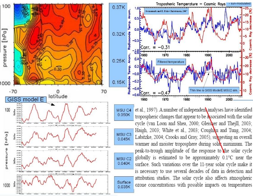
C lim ate C h an g e a nd I t s C a u s e s: A Di s c u s si on A b out S o m e K e y I s s u e s .............3-28
Introduction …............................................................................................................ 4
The IPCC’s pro-anthropogenic warming bias ….......................................................... 6
The climate sensitivity uncertainty to CO2 increase …............................................... 8
The climatic meaning of Mann’s Hockey Stick temperature graph …....................... 10
The climatic meaning of recent paleoclimatic temperature reconstructions …........ 12
The phenomenological solar signature since 1600 …............................................... 14
The ACRIM vs. PMOD satellite total solar irradiance controversy …......................... 16
Problems with the global surface temperature record ….......................................... 18
A large 60 year cycle in the temperature record ….................................................. 19
Astronomical origin of the climate oscillations …..................................................... 22
Conclusion …............................................................................................................ 26
Bibliography …......................................................................................................... 27
A p pendix...................................................................................................................29-54
A: The IPCC’s anthropogenic global warming theory …................................................. 29
B: Chemical vs. Ice-Core CO2 atmospheric concentration estimates …......................... 30
C: Milky Way’s spiral arms, Cosmic Rays and the Phanerozoic temperature cycles ….. 31
D: The Holocene cooling trend and the millennial-scale temperature cycles …............ 32
E: The last 1000 years of global temperature, solar and ice cover data …................... 33
F: The solar dynamics fits 5000 years of human history …........................................... 34
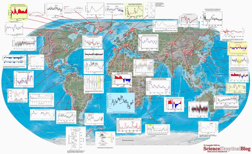
G: The Medieval Warm Period and the Little Ice Age - A global phenomenon …........... 35
H: Compatibility between the AGWT climate models and the Hockey Stick ….............. 36
I: The 11-year solar cycle in the global surface temperature record …........................ 37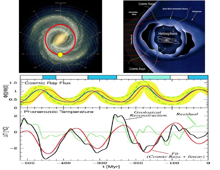
J: The climate models underestimate the 11-year solar cycle signature ….................. 38
K: The ACRIM-PMOD total solar irradiance satellite composite controversy ….............. 39
L: Willson and Hoyt’s statements about the ACRIM and Nimbus7 TSI published data .. 40
M: Cosmic ray flux, solar activity and low cloud cover positive feedback …................. 41
N: Possible mechanisms linking cosmic ray flux and cloud cover formation …............. 42
O: A warming bias in the surface temperature records? ….......................................... 43
P: A underestimated Urban Heat Island effect? …......................................................... 44
Q: A 60 year cycle in multisecular climate records ….................................................... 45
R: A 60 year cycle in solar, geological, climate and fishery records ….......................... 46
S: The 11-year solar cycle and the V-E-J planet alignment …........................................ 47
T: The 60 and 20 year cycles in the wobbling of the Sun around the CMSS ….............. 48
U: The 60 and 20 year cycles in global surface temperature and in the CMSS …......... 49
V: A 60 year cycle in multisecular solar records …........................................................ 50
W: The bi-secular solar cycle: Is a 2010-2050 little ice age imminent? …..................... 51
X: Temperature records do not correlate to CO2 records …........................................... 52
Y: The CO2 fingerprint: Climate model predictions and observations disagree ….......... 53
Z: The 2007 IPCC climate model projections. Can we trust them? …............................ 54
Climate Change and Its Causes
                                   A Discussion About Some Key Issues
                                                       Nicola Scafetta 1,2
                   1
                       Active Cavity Radiometer Irradiance Monitor (ACRIM) Lab, Coronado, CA 92118, USA
                               2
                                   Department of Physics, Duke University, Durham, NC 27708, USA.

Abstract
This article discusses the limits of the Anthropogenic Global Warming Theory advocated by the Intergov-
ernmental Panel on Climate Change. A phenomenological theory of climate change based on the physical
properties of the data themselves is proposed. At least 60% of the warming of the Earth observed since 1970
appears to be induced by natural cycles which are present in the solar system. A climatic stabilization or
cooling until 2030-2040 is forecast by the phenomenological model.

***************************************************************************************

This work is made of

    • An translation into English of the paper:
      Scafetta N., “Climate Change and Its causes: A
      Discussion about Some Key Issues,” La Chimica
      e l’Industria 1, p. 70-75 (2010);

    • Several additional supporting notes are added to the
      paper;

    • An extended appendix section part is added to cover
      several thematic issues to support particular topics
      addressed in the main paper.

  This work covers most topics presented by Scafetta at a seminar at the U.S. Environmental Protection Agency, DC
USA, February 26, 2009. A video of the seminar is here:
http://yosemite.epa.gov/ee/epa/eed.nsf/vwpsw/360796B06E48EA0485257601005982A1#video

The Italian version of the original paper can be downloaded (with possible journal restrictions) from
http://www.soc.chim.it/files/chimind/pdf/2010/2010 1 70.pdf

Preprint submitted to Science & Public Policy (SPPI)                                                      March 4, 2010
Figure 1: Global surface temperature (land and sea) HadCRUT3 (red) and its quadratic fit (black). [Climatic Research Unit,
http://www.cru.uea.ac.uk/].

1. Introduction

   Since 1900 the global surface temperature of the Earth has risen by about 0.8 oC (Fig-
ure 1), and since the 70s by about 0.5 oC. This temperature increase occurred during a
significant atmospheric concentration increase of some greenhouse gases, especially CO2
and CH4 , which is known to be mainly due to human emissions. According to the Anthro-
pogenic Global Warming Theory (AGWT) humans have caused more than 90% of global
warming since 1900 and virtually 100% of the global warming since 1970 (Appendix A).
The AGWT is currently advocated by the Intergovernmental Panel on Climate Change
(IPCC) [1], which is the leading body for the assessment of climate change established by
the United Nations Environment Programme (UNEP) and the World Meteorological Orga-
nization (WMO). Many scientists believe that further emissions of greenhouse gases could
endanger humanity [2].

   However, not everyone shares the IPCC’s views [3].1 More than 30,000 scientists in
America (including 9,029 PhDs) have recently signed a petition stating that those claims
are extreme, that the climate system is more complex than what is now known, several

   1
    The AGWT advocates claim that there exists a scientific consensus that supports the AGWT. However, a scientific consensus
does not have any scientific value when it is contradicted by data. It is perfectly legitimate to discuss the topic of manmade global
warming and closely scrutinize the IPCC’s claims. Given the extreme complexity of the climate system and the overwhelming
evidence that climate has always changed, the AGWT advocates’ claim that the science is settled is premature in the extreme.
                                                                 4
Figure 2: List of radiative forcings held responsible for the global warming since 1750 and used in the models adopted by the IPCC.
The figure is adapted from the IPCC Climate Change 2007: Synthesis Report. These forcings are used as inputs of the climate
models used by the IPCC to support the AGWT. The table suggests that the total net anthropogenic forcing since 1750 has been
13.3 times larger than the natural forcing. However, labeling on the left of the table, anthropogenic and natural, is misleading
because it would imply that only human activity can change the chemistry of the atmosphere, which is non physical.

mechanisms are not yet included in the climate models considered by the IPCC and that
this issue should be treated with some caution because incorrect environmental policies
could also cause extensive damage [3]. This article briefly summarizes some of the rea-
sons, mostly derived from my own research, why the science behind the IPCC’s claim is
questionable.2

   2
     On November 19, 2009 a climategate story erupted on the web. This story is seriously undermining the credibility of the
AGWT and of its advocates. Thousands of e-mails and other documents were disseminated via the internet through the hacking
of a server used by the Climatic Research Unit (CRU) of the University of East Anglia in Norwich, England. These e-mails
have been interpreted by some as suggesting serious scientific misconduct and even conspiracy by leading climate scientists and
IPCC authors who have strongly advocated AGWT. These emails apparently suggest: 1) manipulation of temperature data; 2)
prevention of a proper scientific disclosure of data and methodologies; 3) attempts to discredit scientists critical of the AGWT
also by means of internet articles such as those at http://www.realclimate.org (several of these realclimate.org articles are quite
shallow and suspiciously inaccurate); 4) attempts to bias Wikipedia articles in favor of the AGWT; 5) and much more seriously,
attempts to control which papers appear in the peer reviewed literature and in the climate assessments in such a way to bias the
scientific community in favor of the AGWT. Others, however, believe that the contents of those emails have been maliciously
misinterpreted by the so-called skeptics. A detailed analysis of these emails can be found in: 1) J. P. Costella (2010), Climategate
analysis, SPPI reprint series, (http://scienceandpublicpolicy.org/reprint/climategate analysis.html); 2) S. Mosher and T. W. Fuller
(2010), Climategate: The Crutape Letters, CreateSpace publisher; 3) See also United States Senate Report ‘Consensus’ Exposed:
The CRU Controversy, http://epw.senate.gov/public/index.cfm?FuseAction=Files.View&FileStore id=7db3fbd8-f1b4-4fdf-bd15-
12b7df1a0b63

                                                                 5
2. The IPCC’s pro-anthropogenic warming bias

       First, it should be noted that the IPCC mission states:
         “The IPCC reviews and assesses the most recent scientific, technical and socio-
         economic information produced worldwide relevant to the understanding of human-
         induced climate change.”
The above statement implies that the IPCC may provide a colored reading of the scientific
literature by stressing those studies that would better justify its own political mission, which
evidently focuses on human-induced climate change.3

   Indeed, the existence of an anthropogenic bias appears evident in Figure 2 that shows the
complete list of the radiative forcings, which, as the IPCC claims, have caused the global
climate warming observed since 1750. This figure divides the climatic forcings into two
groups: one group includes only the total solar irradiance and is labeled natural, the other
group comprises the rest and is labeled anthropogenic. Thus, the IPCC claims that 100%
of the increase of the CO2 and CH4 atmospheric concentrations observed since 1750 and
the change of all other climate components, except for the total solar irradiance, are anthro-
pogenic. These labels do suggest that without humans the chemical concentrations of the
atmosphere and a number of other climatic parameters would remain rigorously unchanged
despite a change of the solar energetic input!

   This claim is non physical because as the solar activity increases, climate warms, and
this causes a net increase of atmospheric CO2 and CH4 concentration. During warming the
ability of the ocean to absorb these gases from the atmosphere decreases because of Henry’s
law and other mechanisms. A warming would also increase the natural production of at-
mospheric CO2 and CH4 on the land due to the acceleration of the fermentation of organic
material, outgassing of (permafrost) soils and other mechanisms [3,4]. The existence of
CO2 and CH4 feedback mechanisms are evident in the large CO2 and CH4 cycles observed
during the ice ages (which were caused by the astronomical cycles of Milankovich) when

   3
      Further evidence of the IPCC’s anthropogenic and political bias was discovered in January 2010: the IPCC’s claim that Hi-
malayan glaciers will disappear by 2035 was based on magazine interviews, not on peer-reviewed scientific research which is
contrary to the IPCC’s own policy. Dr. Lal admitted that this physically impossible event was highlighted in the IPCC report
just to put political pressure on world leaders (http://www.dailymail.co.uk/news/article-1245636/Glacier-scientists-says-knew-data-
verified.html). Curiously, NASA anticipated the Himalayan glacier melting to 2030 (http://wattsupwiththat.com/2010/01/23/nasa-
climate-page-suckered-by-ipcc-deletes-a-moved-up-glacier-melting-date-reference/). Other significant errors and non peer-
reviewed material in the IPCC have been uncovered such as: Endanger 40 percent of Amazon rainforests; Melt mountain ice
in the Alps, Andes, and Africa; Deplete water resources for 4.5 billion people by 2085, neglecting to mention that global warming
could also increase water resources for as many as 6 billion people; Slash crop production by 50 percent in North Africa by 2020.
http://epw.senate.gov/public/index.cfm?FuseAction=Files.View&FileStore id=9cc0e46e-56be-4728-9099-92dbda199bfc

                                                                6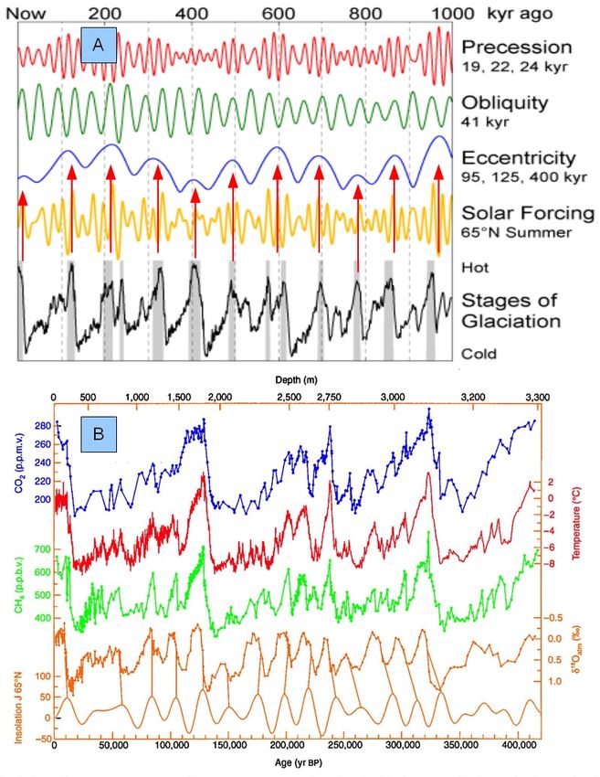
Figure 3: Cycles of CO2 and CH4 that time-lag (with a delay of about 800 years) the temperature cycles observed during the Ice
Ages. These glacial cycles were likely induced by the modulation of the solar input into the Earth’s system through the Milankovich
cycles, which are orbital perturbations of the Earth such as the precession, obliquity and eccentricity. For example, notice the good
correspondence between the 100.000 year temperature cycles with the eccentricity, as highlighted in the figure. The figure is
adapted from Wikipedia’ articles: [A] Milankovitch cycles; [B] Vostok Station.

                                                                 7
no human industrial activity existed, see Figure 3.

    For example, even assuming that the IPCC’s forcing estimates in Figure 2 are correct, if
only 10% of the total increase in greenhouse gases since 1750 has been due to the observed
increase of solar activity during the same period, the IPCC, with its labels, has inflated the
anthropogenic contribution by 20% and underestimated the solar contribution by 300%.4
This can be easily extrapolated from the numbers depicted in Figure 2. It is evident that
if the climatic forcings are labeled as anthropogenic, the presumed consequences, namely
climate changes, would also be anthropogenic. This, however, is circular logic.

3. The climate sensitivity uncertainty to CO2 increase

   A second fundamental issue concerns how much global warming can be induced by an
increase of CO2 (or CH4 ) atmospheric concentration. Indeed, this estimate is extremely
uncertain. Also the radiative forcing associated with aerosols is extremely uncertain, as
Figure 2 shows.

    The IPCC acknowledges that if the atmospheric concentration of CO2 doubles the global
average temperature could rise between 1.5 and 4.5 oC at equilibrium. The variability of
climate sensitivity to CO2 is shown in Figure 4, which demonstrates an even wider sensitiv-
ity temperature range [5]. If greenhouse gases such as CO2 are the major causes of global
warming, a climate sensitivity to CO2 increase with a minimum error of 50% (together with
the extreme aerosol forcing uncertainty) can only raise strong doubts about the scientific ro-
bustness of the IPCC’s climate change interpretation. This error is so large because it is not
well known how to model the major climate feedback mechanisms, i.e., water vapor and
clouds.

   Indeed, the AGWT advocates acknowledge that the current models on which the claims
of the IPCC are based are significantly incomplete. Rockstrom and 28 other scientists [2],
who strongly promote the AGWT, have confirmed this fact by recently stating:

   4
     A recent study (using CO2 ice core reconstructions) found a CO2 feedback rate of 1.7-21.4 ppmv CO2 increase per oC, while
other theoretical and empirical studies found a larger value (Frank D. C. et al. (2010), Ensemble reconstruction constraints on the
global carbon cycle sensitivity to climate, Nature 463, 527-530). However, a comparison between global temperature from 1860
and atmospheric CO2 measurements by direct chemical analysis (not by ice core sample reconstruction) shows an atmospheric
CO2 concentration curve, with a maximum in 1942, which correlates relatively well with the temperature record; both curves
present a maximum in 1940-1945 (Appendix B). This result would indicate the existence of strong CO2 feedback mechanisms,
which would imply that the observed CO2 concentration increase during the last decades is highly related to some carbon cycle
feedback mechanism in response to the increased solar input during this same period. It appears that it is climate change that alters
the atmospheric CO2 concentration, rather than vice versa. [E.-G. Beck (2007), 180 Years of atmospheric CO2 Gas Analysis by
Chemical Methods, Energy & Environment 18, 259-282. http://www.biomind.de/realCO2/realCO2-1.htm ]
                                                                 8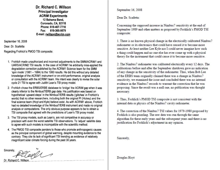
Figure 4: Climate sensitivity to CO2 doubling in function of the feedbacks (from Knutti and Hegerl [5]). Note the large uncertainty:
a CO2 doubling may cause a global warming from 1 oC to 10 oC at equilibrium. The figure on the left explains why there exists
such a large error. The GHG warming theory is based on two independent chained theories. The first theory focuses on the warming
effect of a given GHG such as CO2 as it can be experimentally tested. This first theory predicts that a CO2 doubling causes a global
warming of about 1 oC. The second theory, the climate positive feedback theory, attempts to calculate the overall climatic effect of
a CO2 increase by assuming an enhanced warming effect due to secondary triggering of other climatic components. For example,
it is supposed that an increase of CO2 causes an increase in water vapor concentration. Because H2 O too is a GHG, the overall
warming induced by an increase of CO2 would be due to the direct CO2 warming plus the indirect warming induced by the water
vapor feedback responding to the CO2 increase. The problem with the climate positive feedback theory is that it cannot be directly
tested in a lab experiment. Climate modelers evaluate the climate sensitivity to CO2 increase in their climate models, not in nature.
Thus, the numerical value of this fundamental climatic component is not experimentally measured but it is theoretical evaluated
with computer climate models that create virtual climate systems. It is evident that different climate models predict a different
climate sensitivity to CO2 , which gives rise to the huge uncertainty seen in the figure. Moreover, if the climate models are missing
important mechanisms, it is evident that their predicted climate sensitivity to CO2 changes may be extremely different from the
true values. The left figure is partially adapted from “Catastrophe Denied: A Critique of Catastrophic Man-Made Global Warming
Theory” by Warren Meyer, Phoenix Climate Lecture, November 10 (2009) http://www.climate-skeptic.com/phoenix

                                                                 9
“Most models suggest that a doubling in atmospheric CO2 concentration will
lead to a global temperature rise of about 3 oC (with a probable uncertainty
range of 2-4.5 oC) once the climate has regained equilibrium. But these models
do not include long-term reinforcing feedback processes that further warm the
climate,... If these slow feedbacks are included, doubling CO2 levels gives an
eventual temperature increase of 6 oC (with a probable uncertainty range of 4-8
o
C).”
Rockstrom et al. [2] gave a quite alarmist interpretation to their acknowledgment that
current climate models are missing important feedback mechanisms. However, such alarmism
is baseless.5 In fact, if missing feedback mechanisms were added to the current climate
models, the corrected models would predict a much greater warming than the 0.8 oC ob-
served during the last century. Thus, these models would severely fail to reproduce the
warming of 0.8 oC observed in the temperature data. If the current IPCC climate models
do not contain many feedback mechanisms that amplify the effect of a climate radiative
forcing, the logical conclusion would be that the climate sensitivity to atmospheric CO2
concentration is currently significantly overestimated by those models, while the effect of
the solar input is severely underestimated.
4. The climatic meaning of Mann’s Hockey Stick temperature graph
Let us clarify the issue from a historical perspective. In 1998 and 1999 Mann et al. [6]
published the first reconstruction of global temperature over the last 1000 years. This pale-
oclimatic temperature reconstruction is known as the Hockey Stick (Figure 5). This graph
suggests that before 1900 the temperature of the planet was almost constant and since 1900
an abnormal warming has occurred. From the Medieval Warm Period (1000-1300) and the
Little Ice Age (1500-1750) this reconstruction predicts a cooling of less than 0.2 oC. This
graph surprised many, including historians and geologists who have consistently argued
that the early centuries of the millennium were quite warm (the Medieval Warm Period)
while the period from 1500 to 1800 was quite cold (the Little Ice Age).6
5
Rockstrom et al. [2] have implicitly acknowledged that the IPCC climate models are essentially flawed. This objectively
undermines the IPCC’s claims because its claims are based on the same climate models that the AGWT advocates acknowledge to
be severely incomplete. Evidently, Rockstrom et al.’s claim that future climate models will necessarily confirm and greatly stress
the AGWT cannot be considered as a fact. Indeed, it cannot be ruled out that, on the contrary, future climate models will discredit
the AGWT by modeling new climate mechanisms that current models lack.
6
This larger climate variability was clearly acknowledged by the IPCC in 1990. It was also consistent with the world climate
history after AD 1,000 according to ground borehole evidence in a paper published in 1997 (Huang S. H. N. Pollack and P. Y. Shen
(1997), Late Quaternary Temperature Changes Seen in Worldwide Continental Heat Flow Measurements, Geophysical Research
Letters 24, 1947-1950.)
10Figure 5: (Red) Mann’s Hockey Stick [6]. (Blue) Output response of Crowley’s linear upwelling/diffusion energy balance model
using all forcing terms (solar, volcano, CO2 and aerosol) [7]. Instrumental temperature data (black). Note the very good agreement
between the model and temperature reconstruction that is claimed by Crowley in his article. Note that from the Medieval Warm
Period (1000-1300) to the Little Ice Age (1500-1750) both the model response and Mann’s temperature reconstruction show a
cooling of about 0.2 oC.
The Hockey Stick temperature graph was considered the only global temperature re-
construction available at the time and it required a scientific interpretation. Several scien-
tific groups, for example Crowley [7], used energy balance models and concluded that the
Hockey Stick implied that the climate is almost insensitive to solar changes and the anoma-
lous warming observed since 1900 has been almost entirely anthropogenic. In fact, only the
(CO2 and CH4 ) GHG forcing function (as deduced from ice core reconstructions) presents
a shape that resembles that of a hockey stick. Crowley concluded his article, which shows
a good correlation between his climate model and the Hockey Stick, with this statement:
“The very good agreement between models and data in the pre-anthropogenic
interval also enhances confidence in the overall ability of climate models to sim-
ulate temperature variability on the largest scales.” (See Figure 5)
Crowley’s statement reveals the subtle link that exists between the Hockey Stick and the
confidence in the sufficient accuracy of the climate models used to claim that the global
warming observed since 1900 was almost entirely anthropogenically induced. This inter-
pretation was strongly endorsed by the IPCC in 2001, was popularized by Al Gore in his
documentary The Inconvenient Truth, where the Hockey Stick plays a predominant role,
and was almost completely implicitly proposed again by the IPCC in 2007. It is important
11Figure 6: Top: Moberg’s temperature (red) [8]. Crowley’s model (blue) [7] which is also shown in Figure 5. Bottom: In blue
Crowley’s model once adapted to reproduce the temperature of Moberg et al. (2005) that shows a 0.6 oC cooling from MWP and
LIA. Note that the solar contribution must be amplified by a factor of 3 while the GHG+aerosol contribution, which is commonly
labeled as anthropogenic, must be reduced to a factor of 0.4.
to note that the IPCC’s AGWT is based on the interpretation of climate models, such as
Hansen’s GISS models [20], developed before 2004/5 which appear to be compatible with
the Hockey Stick temperature graph (see also Appendix H).7
5. The climatic meaning of recent paleoclimatic temperature reconstructions
The dates are important because since 2004/2005 the Hockey Stick has been mathemati-
cally and physically questioned.8 An additional open issue is whether the tree rings used by
7
For example, the GISS GCM are compared and found relatively compatible with Mann’s Hockey Stick temperature graph
in Shindell D.T., G.A. Schmidt, R.L. Miller, and M.E. Mann, (2003), Volcanic and solar forcing of climate change during the
preindustrial era. J. Climate 16, 4094-4107. A compatibility with the Hockey Stick temperature graph is also easily visible in
the energy balance model (EBM) simulations in Foukal P., C. Fröhlich, H. Spruit, T. M. L. Wigley (2006), Variations in solar
luminosity and their effect on the Earth’s climate, Nature 443, 161-166. In this paper it is clear that the EBM model simulations
predict a cooling between the Medieval Warm Period (1000-1300) and the Little Ice Age (1500-1800) of less than 0.2 oC as shown
by Mann’s Hockey Stick.
8
The problems with Mann’s original Hockey Stick temperature graph were first exposed by McIntyre and McKitrick (2005),
The M&M Critique of the MBH98 Northern Hemisphere Climate Index: Update and Implications, Energy and Environment 16(1),
69-100. It was shown than Mann’s algorithm could produce hockey stick shapes even with a set of red noise sequences. Note that
recently Mann has updated his reconstruction and acknowledged that the preindustrial temperature varied more than previously
claimed in his works (Mann M. E., et al. (2008), Proxy-based reconstructions of hemispheric and global surface temperature
variations over the past two millennia, Proc Natl Acad Sci USA 105, 13252-13257). However, McIntyre and McKitrick have claimed
that also this latest Mann’s update presents significant mathematical errors including some records that would be improperly used
12Mann are able to accurately reconstruct the temperature changes, especially over long time
scales. Indeed, tree growth does not depend on temperature alone but on other factors too,
such as rain patterns and biological adaptation. These multiple factors may introduce non-
linear relationships and a certain degree of randomness in the data. This may reduce the
amplitude of multidecadal and secular oscillations found in the proxy models, in particular
when these proxy records are statistically calibrated against the instrumental temperature
records, which are only available for the period after 1850, and combined for obtaining a
world average.
Alternative paleoclimatic reconstructions, which do not use tree rings, have been pro-
posed [8-10]. These proxy temperature reconstructions suggest a significant pre-industrial
climate variability. From the Medieval Warm Period (1000-1300) and the Little Ice Age
(1500-1750) these reconstructions show a cooling of at least 0.6 oC, three times larger
than the Hockey Stick. Figure 6 shows that if Crowley’s energy balance model is com-
pared against Moberg’s paleoclimatic temperature reconstruction [8], Crowley’s very good
agreement between the model and the data vanishes. If Crowley’s model is recalibrated to
reconstruct Moberg’s temperature, it is easy to calculate that the solar effect must be ampli-
fied by a factor of 3 and the anthropogenic effect (GHG + Aerosol) should be multiplied by
0.4. Thus, if Moberg’s temperature is accurate, in 2000 the anthropogenic contribution to
global warming was overestimated by 250% because of the Hockey Stick.
Indeed, the Hockey Stick temperature graph does not have any historical credibility be-
cause between 1000 and 1400, the Vikings had farms and villages on the coast of Greenland,
which would suggest an even milder climate than today, while the following period, from
1400 to 1800, is known as the Little Ice Age. The medieval warm and the following cold
period were not only Western and European phenomena but are also evident in Chinese
historical documents [11]. Numerous interdisciplinary studies reporting data from several
regions of the world (see the Medieval Warm Period Project9 ) clearly indicate a signifi-
cant change in pre-industrial climate which seems to be better reproduced by more recent
paleoclimatic global temperature reconstructions [8-10] which do not show a hockey stick
shape.10 See Appendixes C-H for further details about climate data at multiple time scales.
with the axes upside down by Mann’s algorithm because these records are severely compromised by agricultural impact during
the last century, e.g., Korttajarvi sediments from Tiljander data. Therefore, these data could not be used for reconstructing the
past temperature because they could not be properly calibrated against the instrumental temperature record. (McIntyre S. and R.
R. McKitrick (2009) Proxy Inconsistency and Other Problems in Millennial Paleoclimate Reconstructions. Proc Natl Acad Sci
USA 106, E10.). See an extended comment by McIntyre here: http://climateaudit.org/2009/10/14/upside-side-down-mann-and-the-
peerreviewedliterature/. Also interesting is the following comment by Eschenbach: http://climateaudit.org/2008/11/23/cant-see-
the-signal-for-the-trees/
9
http://www.CO2 science.org/data/mwp/mwpp.php
10
A nice summary about the findings of numerous studies published before and after Mann’s original work in 1998 and 1999 that
13Figure 7: Reconstruction of global surface temperatures over the last 400 years (red and green). In black there is the solar signature
on climate as estimated by the empirical model [12]. If since 1980 the TSI satellite composite A in figure 8 (PSS # 1) is used most
of the warming observed during the last decades is solar induced. If the TSI satellite composite C in figure 8 (PSS # 2) is used the
good correlation between temperature and solar signature abruptly stops in 1980. (Appendix I)
6. The phenomenological solar signature since 1600
It is possible to use a phenomenological model to interpret climate change [12]. This
model can simulate a typical energy balance model to interpret the global surface tem-
perature. However, here the climate sensitivity to solar variations and the thermodynamic
characteristic relaxation times are empirically determined in the temperature patterns dur-
ing the last decades. A secular total solar irradiance reconstruction is used as input of the
model as a proxy for the total solar activity. The model can be used to reconstruct the so-
lar signature on climate for the past centuries and it is possible to compare this signature
against the paleoclimatic temperature reconstructions. Figure 7 shows this result: the tem-
perature signature induced by solar changes as predicted by the phenomenological model
well reproduces 400 years of climate change as reconstructed by Moberg et al. [8].
The advantage of the phenomenological approach over that implemented in the tradi-
tional climate models, which can be described as analytic engineering, is that the phe-
nomenological approach attempts to measure the climate sensitivity to solar changes through
strongly question the validity of the Hockey Stick temperature graph can be found in Heaven and Earth, Global Warming the Missing
Science, chapter 2 ‘History,’ by Ian Plimer, Taylor Trade (2009). Apparently, the IPCC’s choice in 2001 to strongly highlight Mann’s
Hockey Stick temperature graph, despite extensive published literature pointing toward a large preindustrial climate variability, can
be interpreted as a further evidence of the IPCC’s pro-anthropogenic warming bias, as discussed in Section 2.
14the empirical determination of a kind of response function. This methodology would take
into account all mechanisms involved in the process, although the individual microscopic
mechanisms are not explicitly modeled. It is essentially analogous to the method used by
an electric engineer to study the electric response properties of an unknown circuit closed
inside a box by carefully comparing the patterns of the input and the output signals. The
phenomenological approach is essentially a holistic approach 11 that emphasizes the im-
portance of studying a complex macroscopic system by directly analyzing the properties of
the whole because of the complex interdependence of its parts rather than analyzing it by
separating it into parts.
On the contrary, the traditional analytic climate model approach attempts to simulate
climate by dividing the climate system into its smallest possible or discernible elements
and uses their elemental physical properties alone to interpret the macroscopic system. The
limitation of the latter approach is that only those mechanisms and the physical couplings
among them that are currently well known can be modeled. All unknown mechanisms and
physical couplings remain excluded in an analytic model. Therefore, the analytic modu-
larization may fail to properly model and interpret climate change because it just creates
a virtual climate system that may have nothing to do with reality. The risk is scientific
reductionism, that is, compensating the current ignorance about the true climatic mecha-
nisms by mistakenly stressing a few of them, such as the anthropogenic GHG and aerosol
forcings, in such a way to reproduce some warming trend during a restricted period of
time. However, for not mistaking the physics of a complex phenomenon a model should
be able to reproduce the data oscillations at multiple time scales. In science, the holistic
approach complements the traditional analytical approach. When the two methodologies
are appropriately used together, they are considered the most efficient way for studying
complex systems. Essentially, the phenomenological approach acknowledges that under-
standing climate is an inverse-problem that risks to be ill-posed in the analytic approach.
For example, the IPCC [1, p. 674] reports that the 11-year solar cycle produces a temper-
ature cycle on the global surface temperature of about 0.1 oC that is easy to observe [12].
However, current climate models predict an average solar signature cycle which is three
times smaller, approximately 0.035 oC [12] (for example, Crowley’s model [7] predicts a
cycle of about 0.02 oC). It is obvious that the current climate models are oversimplified.
They are poorly modeling the solar-climate link mechanisms and, therefore, mistaking the
real magnitude of the solar effects on climate (Appendix J).
11
The term holistic science is used as a category encompassing a number of scientific research fields. These are multidisciplinary,
are concerned with the behavior of complex systems, and recognize feedback within systems as a crucial element for understanding
their behavior. http://en.wikipedia.org/wiki/Holism in science
15In fact, the IPCC models assume that the sun can influence climate only through total
solar irradiance variation, that is used only as a radiative forcing. However, there are addi-
tional chemical mechanisms that are stimulated by specific frequencies of the solar radiation
(for example, UV alters ozone, which is a greenhouse gas, and light stimulates photosynthe-
sis which influences the biosphere) and there is an additional modulation of clouds, which
alters the albedo, that is due to the solar modulation of cosmic ray flux [13,14].12 All these
alternative solar-climate link mechanisms are absent in the current climate models because
the climate modelers do not know how to model them and the computers are not sufficiently
fast to simulate them. The phenomenological model would automatically include all these
mechanisms because the climate sensitivity to solar changes is directly, that is phenomeno-
logically, estimated by the magnitude of the temperature patterns that can be recognized as
correlated to and, therefore, likely induced by solar changes.
7. The ACRIM vs. PMOD satellite total solar irradiance controversy
Some discrepancy between the temperature reconstruction and the solar signature on
climate as seen in Figures 6 and 7 may also be due to errors in the temperature as well
as in the solar proxy records. Figure 7 shows two possible empirical solar signatures on
climate after 1980. This uncertainty is due to an uncertainty about the behavior of the total
solar irradiance. The climate models adopted by the IPCC have used total solar irradiance
(TSI) proxy models that claim that total solar irradiance has remained constant since 1980.
However, the satellite experimental groups (ACRIM and Nimbus7), which have measured
the total solar irradiance since 1978, claim that TSI increased from 1980 to 2000 like the
temperature [15].13
12
A solar induced low cloud cover modulation can greatly affect climate by greatly enhancing the climatic solar impact because
of the potential magnitude of the resulting radiative forcing. This is evident from the fact that cloudy days are significantly cooler
than sunny days. In fact, if clouds were absent the solar radiative forcing warming the Earth’s surface would increase by about
30 W/m2 . This value is far larger than the sum of all IPCC anthropogenic forcings in 250 years shown in Figure 2. Thus, even
a small solar modulation of cloud cover can have a significant impact on climate change. Clouds can also respond quite fast to
cosmic ray flux variations and, therefore, they may link some temperature fluctuations to the solar intermittency. Finally, a cosmic-
ray cloud climate link has been suggested to explain the warm and ice periods of the Phanerozoic during the last 600 million
years. In fact, the climate oscillations correlate with the cosmic ray flux variations much better than with the CO2 atmospheric
concentration records. In the latter case, most of the cosmic ray flux variation is claimed to be due to the changing galactic
environment of the solar system, as it crosses the spiral arms of the Milky Way (Shaviv, N. J. (2003), The spiral structure of
the Milky Way, cosmic rays, and ice age epochs on Earth, New Astronomy 8, 3977; Svensmark H. (2007), Cosmoclimatology:
a new theory emerges, Astronomy & Geophysics 48 1, 18-24; Kirkby J. (2009), Cosmic rays and climate, CERN Colloquium,
http://indico.cern.ch/getFile.py/access?resId=0&materialId= slides&confId=52576)
13
Although it is not possible to verify the accuracy of all satellite measurements, to claim that the TSI proxy models must
necessarily be correct is scientifically unsound. TSI proxy models, by definition, are based on the unproven assumptions that a
given set of solar related measurements (such as sunspot number records, a few ground based spectral line width records, 14C and
10
Be cosmogenic isotope production and others) can reconstruct TSI. However, TSI proxy models significantly differ from each
other and, evidently, this undermines the claim that they are accurate. Thus, although TSI proxy models are useful, they cannot be
used to question the accuracy of actual TSI satellite measurements without valid physical reasons. Some of the more popular TSI
proxy models were produced by Lean et al., Solanki et al. and Hoyt and Schatten.
16Figure 8: Possible reconstructions of the total solar irradiance using satellite data [12]. The reconstruction ‘A’ uses the Nim-
bus7/ERB dataset to fill the ACRIM-gap from 1989.5 to 1991.75; the reconstruction ‘C’ uses the ERBE/ERBs dataset to adjust the
annual trend of the Nimbus7/ERB dataset and uses this altered record to fill the ACRIM-gap from 1989.5 to 1991.75; the recon-
struction ‘C’ is jus the average between the two. The level difference between the minimum in 1986 and 1996 is approximately
0.3 ± 0.4W/m2 . ACRIM is between ‘A’ and ‘B’; PMOD is similar to ‘C’. The red curves indicate the trend between the 1986 and
1996 solar minima.
However, another group, the PMOD in Switzerland, claimed that the TSI satellite data
obtained and published by the above two experimental groups had to be corrected.14 By
doing so, Fröhlich obtained a TSI satellite composite that does not show any upward trend
from 1980 to 2000 [16]. It is important to notice that the experimental groups have always
rejected the corrections of their own TSI data proposed by PMOD as arbitrary [15].15
14
During the ACRIM-gap (1989.5-1992.5) Fröhlich [16] altered the Nimbus7/ERB results to make them compatible with the
ERBE/ERBS results. The Nimbus7 record was shifted downward by 0.86 W/m2 . This shift consisted of: (1) a step function change
of about 0.47 W/m2 which is used to correct a hypothetical sudden change of the sensitivity of the Nimbus7’s sensors following a
shutdown claimed to have occurred on 09/29/1989; (2) a linear drift of 0.142 Wm−2 /yr from October 1989 through middle 1992
which is supposed to correct an hypothetical gradual sensitivity increase of the same satellite sensors. However, during the ACRIM-
gap ERBE/ERBS sensors were expected to degrade due to a decrease in their cavity paint absorbency which occurs during the first
exposure of these kind of sensors to high solar maximum UV radiation. So, the experimental teams claim that Fröhlich’s alteration
of the published Nimbus7/ERB data, to force them to agree with the lower quality ERBE/ERBS results, is unjustified.
15
On September 16, 2008, Douglas Hoyt (PI of the Nimbus7/ERB experiment which is fundamental for resolving the ACRIM-
gap problem, and whose data have been altered to construct the PMOD TSI satellite composite) sent me the following statement
that was published in Ref. [15]: “Concerning the supposed increase in Nimbus7 sensitivity at the end of September 1989 and
other matters as proposed by Fröhlich’s PMOD TSI composite: 1. There is no known physical change in the electrically calibrated
Nimbus7 radiometer or its electronics that could have caused it to become more sensitive. At least neither Lee Kyle nor I could
never imagine how such a thing could happen and no one else has ever come up with a physical theory for the instrument that
could cause it to become more sensitive. 2. The Nimbus7 radiometer was calibrated electrically every 12 days. The calibrations
before and after the September shutdown gave no indication of any change in the sensitivity of the radiometer. Thus, when Bob Lee
of the ERBS team originally claimed there was a change in Nimbus7 sensitivity, we examined the issue and concluded there was
17Figure 9: Left: Global surface temperature records of the ocean and the land. Note the significant difference observed between the
two records since 1970. The land apparently warmed at a double rate than the ocean. Right: Global surface temperature record
relative to the United States of America. Note that this record highlights the existence of a large 60-70 year cycle and shows a
smaller upward secular trend. (GISTEMP: http://data.giss.nasa.gov/gistemp/)
By preferring the PMOD total solar irradiance satellite composite to the ACRIM one the
IPCC message was that the global warming observed since 1980 could not be naturally in-
terpreted and, therefore, it had to be 100% anthropogenic. Figure 8 shows three alternative
reconstructions of the total solar irradiance using satellite measurements since 1978. The
IPCC has adopted a reconstruction similar to C, which is compatible with PMOD’s claim.
However, the figure clearly indicates that the latter composite shows the lowest 1986-1996
decadal trend but, as the figure suggests, total solar irradiance could very likely have in-
creased from 1980 to 2000 (See also Appendixes K-N).
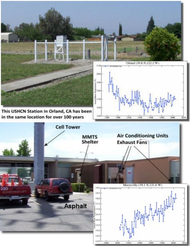
8. Problems with the global surface temperature record
Once again it is the uncertainty in the data that makes it difficult to correctly interpret
climate change. Even the global warming of about 0.8 oC since 1900 may be uncertain. In
fact, during this period the land warmed by about 1.1 oC, while the oceans warmed by about
0.6 oC (Figure 9). This difference appears to be too significant to be explained only by the
no internal evidence in the Nimbus7 records to warrant the correction that he was proposing. Since the result was a null one, no
publication was thought necessary. 3. Thus, Fröhlich’s PMOD TSI composite is not consistent with the internal data or physics of
the Nimbus7 cavity radiometer. 4. The correction of the Nimbus7 TSI values for 1979-1980 proposed by Fröhlich is also puzzling.
The raw data was run through the same algorithm for these early years and the subsequent years and there is no justification for
Fröhlich’s adjustment in my opinion.”
18different thermal inertia between the ocean and the land regions. It could be partially due
to an underestimation of the urban heat island effect by at least 10-20% [17], to land use
changes or perhaps to the fact that several meteorological stations located in cold regions
were closed after 1960.16 The US temperature record present a smaller warming trend since
1880 than the global temperature records. Given the better quality of this record, this find-
ing may suggest that part of the reported global warming may be spurious. If the warming
trend has been overestimated (or if it was partially due to land use changes), the effect of
CO2 and CH4 on climate change has to be reduced for this reason as well (Appendix O-P).
9. A large 60 year cycle in the temperature record
A reasonable alternative is to extract any relevant physical information from the tem-
perature fluctuations. It has been observed that several multi-secular climatic and oceanic
records present large cycles with periods of about 50-70 years with an average of 60 years
[18].17 Figure 10 shows the global temperature record detrended of its quadratic upward
trend [19] depicted in Figure 1. This sequence has been filtered of its fast fluctuations (by
applying a six year moving average smooth algorithm) and it has been plotted against itself
with a time-lag of about 60 years. The figure clearly suggests the existence of an almost
perfect cyclical correspondence between the periods 1880-1940 and 1940-2000. The peak
in 1880 repeats in 1940 and again in 2000. The smaller peak in 1900 repeats in 1960. This
60-odd year oscillation cannot be associated with any known anthropogenic phenomenon
[19]. (See also Appendixes Q and R).
On the contrary, Figure 11 shows the global temperature as reproduced by a typical cli-
mate model such as the GISS ModelE [20], one of the major climate models adopted by
the IPCC 2007. The failure of the model to reproduce the 60 year cycle is evident from the
16
The surface temperature data present several problems that may have skewed the data so as to overstate the observed warm-
ing trend both regionally and globally. For example, it has been observed that there is a significant divergence between ground
temperature measurements and satellite global temperature measurements (Klotzbach P. J. et al. (2009), An alternative explana-
tion for differential temperature trends at the surface and in the lower troposphere, J. Geophys. Res. 114, D21102.) Possible
causes may be: 1) More than three-quarters of the 6,000 stations that apparently existed in the 60s were discontinued during the
last decades; 2) Higher-altitude, higher-latitude, and rural locations, all of which had a tendency to be cooler, have been tenden-
tiously removed; 3) Contamination by urbanization, changes in land use, improper siting, and inadequately-calibrated instrument
upgrades further overstates warming; 4) Cherry-picking of observing sites combined with interpolation to vacant data grids may
have further stressed heat-island bias; 5) Satellite temperature monitoring findings are increasingly diverging from the station-
based constructions in a manner consistent with evidence of a warm bias in the surface temperature record. For an overview on
this issue see J. D’Aleo J. and A. Watts (2010), Surface Temperature Records: Policy Driven Deception?, SPPI original paper
(http://scienceandpublicpolicy.org/images/stories/papers/originals/surface temp.pdf)
17
Climatic records that present a dominant cycle at about 60 year period include ice core sample, pine tree samples, sardine and
anchovy sediment core samples, global surface temperature records, atmospheric circulation index, length of the day index, etc.
19Figure 10: The 60 year cycle modulation of the temperature [19]. (Red) global temperature detrended of its quadratic upward trend
which is shown in Figure 1. (Blue) the same record time-lag shifted of about 60 years. Note the perfect symmetry between the
periods 1880-1940 and 1940-2000 that excludes the fact that these cycles could have had an anthropogenic origin. Even a smaller
peak in 1900 repeats in 1960. This overwhelming clear finding, by alone, contradicts the AGWT and the IPCC’s claim that 100%
of the warming observed from 1970 to 2000 is anthropogenic.
figure. Indeed, all IPCC climate models have the same failing.18
The existence of a natural 60 year cycle with a total (min-to-max) amplitude of at least
0.3 oC, as Figure 10 shows, implies that at least 60% of the 0.5 oC warming observed since
1970 is due to this cycle. Considering that longer natural cycle can be present and that solar
activity was stronger during the second half of the 20th century than during the its first half
[12], the natural contribution to the warming since 1970 may have been even larger than
60%. Human emissions can have contributed at most the remaining 40%, or less, of the
warming observed since 1970 (if no overestimation of the global warming is assumed as
Section 8 would suggest), not the 100% as claimed by the IPCC. This 60 year cycle has just
entered into its cooling phase and this will likely cause a climate cooling, not a warming,
18
The other IPCC model scenario runs also fail to reproduce this 60-year cycle. These climate model
simulations can be downloaded from the IPCC Data Archive at Lawrence Livermore National Laboratory
(http://climexp.knmi.nl/selectfield co2.cgi?someone@somewhere). However, this is not the only shortcoming of the climate
models adopted by the IPCC. These models have predicted an increase in the warming trend with altitude in the tropic troposphere
due to anthropogenic GHG emissions, but balloon and satellite temperature observations have shown a significant disagreement
with the model predictions. (Douglass D. H., J. R. Christy, B. D. Pearson and S. F. Singer (2007), A comparison of tropical
temperature trends with model predictions, Intl. J. Climatology, DOI: 10.1002/joc.1651). A list of comparison of model predictions
with actual observations and the incompatibility between the two was prepared by Douglas Hoyt: Greenhouse Warming Scorecard
Updated 4/2/2006 (http://www.warwickhughes.com/hoyt/climate-change.htm)
20Figure 11: Global temperature (red) against the temperature prediction of the GISS ModelE [20] adopted by the IPCC. The temper-
ature shows a clear cycle of about 60 years which herein is emphasized by black segments. This 60 year cycle has been explicitly
shown in Figure 10. This cycle is clearly not reproduced by the climate model simulation [19]. The climate simulation clearly
crosses from 1880 to 1970 the black segments instead of reproducing the 60 year modulation of the temperature.
until 2030-40, as Figure 10 would suggest.19
The latter result is quantitatively consistent with the results depicted in Figures 6-8 that
suggest a significant change in pre-industrial climate, in contrast to the Hockey Stick, and
that solar activity has increased from 1980 to 2000 as Willson of the ACRIM team claims
in contrast to PMOD Fröhlich’s claim. In fact, they are consistent with a reduction of the
anthropogenic contribution by 250% as calculated above in Figures 6 and 7. The indepen-
dent results depicted in Figures 6, 7 and 10 are consistent with each other and would imply
that if the CO2 atmosphere concentration doubles, the temperature could rise between 1.0
and 1.5 oC, which is significantly less than the IPCC’s estimate of 1.5-4.5 oC.
This result clearly indicates that the possible impacts that anthropogenic GHGs can have
on global climate change should be greatly diminished. Consequently, the IPCC’s claims
about imminent and catastrophic consequences that human emissions are causing and will
cause, are unsubstantiated: these claims should be greatly moderated. The existence of a
large 60-year natural cycle in the global temperature essentially points toward the conclu-
sion that nature, not human activity, rules the climate.
19
There is strong observational evidence that the ocean has been cooling since 2003 (Loehl C. (2009), Cooling of the global
21Figure 12: Spectral analysis of the global temperature from 1850 to 2009 (above), and of the speed of the center of mass of the solar
system SCMSS (below) [19]. Cycles 5 and 8 are also close to the 11 ± 1 and 22 ± 2 year solar cycles. The M cycle in the spectrum
of the temperature at about 9 year is absent in the SCMSS record. However, it corresponds to a lunar cycle (Appendix Q-W).
10. Astronomical origin of the climate oscillations
If the temperature is characterized by natural periodic cycles the only reasonable ex-
planation is that the climate system is modulated by astronomical cycles. Natural cycles
known with certainty are the 11 (Schwabe) and 22 (Hale) year solar cycles, the cycles of
the planets and luni-solar nodal cycles [19]. Jupiter has an orbital period of 11.87 years
while Saturn has an orbital period of 29.4 years. These periods predict three other major
cycles which are associated with Jupiter and Saturn: about 10 years, the opposition of two
planets; about 20 years, their synodic cycle; and about 60 years, the repetition of the com-
bined orbits of the two planets. The major lunar cycles are about 18.6 and 8.85 years.
Figure 12 shows a spectral analysis of the global surface temperature and of a record that
depends on the orbits of planets (the speed of the sun relative to the center of mass of the
solar system [19]). The two records have almost the same cycles. The temperature record
contains the cycles of the planets combined with the two solar cycles of 11 and 22 years
and a lunar cycle at about 9.1 years.20 (See also Appendixes Q-V).
ocean since 2003, Energy & Environment 20, No. 1&2, 101-104).
20
The temperature cycle ‘M’ shown in Figure 12 appears to be exactly at 9.1 ± 0.1 years. This period is exactly between the
period of the recession of the line of lunar apsides, about 8.85 years, and half of the period of precession of the solar-luni nodes,
about 9.3 years.
22Figure 13: Global temperatures (red) and the reconstruction of temperature using only the 20 and 60 year planetary cycles (in
black). The dashed curve indicates simply the quadratic trend of the temperature [19].
These cycles can be used to reconstruct the fluctuations of the temperature [19]. For
example, it is possible to adopt a model using only the major 20 and 60 year cycles plus a
quadratic trend of the temperature and the reconstruction of Figure 13 is obtained. Other
natural cycles associated with the Sun are evident in Figures 6 and 7. The model recon-
structs with great accuracy the temperature oscillations since 1850. It suggests that until
2030-2040 the temperature may remain stable if the upward trend in temperature observed
from 1850 to 2009 continues in the near future21 or the global temperature cools if the trend
of the secular solar activity decreases, as other independent considerations would suggest.
For example, an imminent relatively long period of low solar activity may be predicted
on the basis that the latest solar cycle (cycle #23) lasted from 1996 to 2009, and its length
was about 13 years instead of the traditional 11 years. The only known solar cycle of com-
parable length (after the Maunder Minimum) occurred just at the beginning of the Dalton
solar minimum (cycle #4, 1784-1797) that lasted from about 1790 to 1830. The solar Dalton
minimum induced a little ice age that lasted 30-40 years as shown in Figure 7. Therefore, it
is possible that the Sun is entering into a multi-decade period of low activity, which could
produce cooling of the climate. (Appendix W).
21
Note that a quadratic trend function supposes a warming acceleration. Even in this situation Figure 13 would suggest that by
2100 the temperature will increase no more than 1 oC above the actual values. This estimate is significantly lower than the IPCC
estimates (their figure SPM.5) that have projected a warming from 1 to 6 oC according to different GHG emission scenarios.
23You can also read