Color Naming Models for Color Selection, Image Editing and Palette Design
←
→
Page content transcription
If your browser does not render page correctly, please read the page content below
Color Naming Models for Color Selection,
                             Image Editing and Palette Design
                              Jeffrey Heer                                                        Maureen Stone
                      Computer Science Department                                                Tableau Software
                           Stanford University                                                     Seattle, WA
                         jheer@cs.stanford.edu                                              mstone@tableausoftware.com

ABSTRACT                                                                             term. Berlin & Kay noted striking regularities among the
Our ability to reliably name colors provides a link between                          use of color terms across cultures, leading them to posit 11
visual perception and symbolic cognition. In this paper, we                          universal basic color terms (in English: blue, brown, green,
investigate how a statistical model of color naming can en-                          orange, pink, purple, red, yellow, black, grey, and white).
able user interfaces to meaningfully mimic this link and sup-                        They observed that these terms were added to a language in
port novel interactions. We present a method for construct-                          a similar progression across cultures. Subsequent decades
ing a probabilistic model of color naming from a large, un-                          of research (e.g., [10, 14, 29, 39]) have challenged and ex-
constrained set of human color name judgments. We de-                                tended this understanding. For example, more than 11 basic
scribe how the model can be used to map between colors and                           color terms may exist (e.g., Russian contains two basic terms
names and define metrics for color saliency (how reliably a                          for blue [39]), and language can have a relative effect on cat-
color is named) and color name distance (the similarity be-                          egorical color perception and memory [29].
tween colors based on naming patterns). We then present
a series of applications that demonstrate how color naming                           The importance of color names to perception and object clas-
models can enhance graphical interfaces: a color dictionary                          sification has led researchers to formulate a variety models
& thesaurus, name-based pixel selection methods for image                            describing how people associate names and colors [2, 8, 20,
editing, and evaluation aids for color palette design.                               22, 24, 26]. Here, we extend prior models — in particular,
                                                                                     the non-parametric approach of Chuang et al. [8] — to pro-
Author Keywords                                                                      pose a model-construction method for a collection of human
Color names; color modeling; palette design; image editing;                          color-name judgments. We then demonstrate how the result-
visualization; perception; XKCD                                                      ing model can be applied to enhance user interfaces. Our
ACM Classification Keywords                                                          research contributions fall into two categories:
H.5.2 Information Interfaces and Presentation: UI
                                                                                     First, we contribute a method for constructing a proba-
                                                                                     bilistic model of color naming from a large, unconstrained
INTRODUCTION                                                                         set of human color name judgments. We model color-name
To reason and communicate about the world, people contin-                            associations using multinomial probability distributions that
ually — and often effortlessly — categorize elements of their                        describe the likelihood of a color value given a color name,
sensory experience. We perceive a world populated by ob-                             or vice versa. We then define useful operations in terms of
jects that we label with named types, colors, shapes, tastes,                        this model. We apply our method to results from a large
odors, and functions. Our capacity for categorization links                          web-based survey [25] containing over 3 million entries and
sensing of the physical world to language and cognition, and                         over 100,000 unique color name responses. Our method in-
underlies our ability to communicate and reference objects                           cludes a scaling technique that reduces this survey data to a
in the world [16]. This observation suggests that user in-                           small set of maximally information-preserving color terms.
terfaces that model human category judgments might enable                            We then describe how the model can be used to map between
more compelling forms of reference and selection.                                    colors and names and we define metrics for color saliency
                                                                                     (how reliably a color is named) and color name distance (the
In this paper, we explore this idea in the domain of color                           similarity between colors based on naming patterns).
names — the linguistic labels used to describe colors. In-
terest in color names as a means to investigate links between                        Second, we present novel interfaces enabled by our color
perception, language, and cognition was spurred by the stud-                         naming model. These applications help users express color
ies of Berlin & Kay [5] in the 1960s. They asked speakers of                         in new ways and offer designers new means for evaluating
various languages to name a set of color stimuli and then se-                        their designs. We describe a color dictionary & thesaurus
lect the most representative stimulus for each provided color                        tool for name-based color selection and browsing of color
                                                                                     synonyms and antonyms. We then describe techniques for
                                                                                     name-based pixel selection for image editing. We introduce
                                                                                     methods to (1) suggest highly-probable color names to de-
Permission to make digital or hard copies of all or part of this work for
personal or classroom use is granted without fee provided that copies are            scribe image pixels, (2) select image regions by color name,
not made or distributed for profit or commercial advantage and that copies           and (3) provide a new “magic wand” tool based on color
bear this notice and the full citation on the first page. To copy otherwise, or      name similarity. Finally, we show how color name overlap
republish, to post on servers or to redistribute to lists, requires prior specific   and saliency statistics supported by our model can aid the
permission and/or a fee.
CHI’12, May 5–10, 2012, Austin, Texas, USA.
                                                                                     design and evaluation of color palettes for visualization.
Copyright 2012 ACM 978-1-4503-1015-4/12/05...$10.00.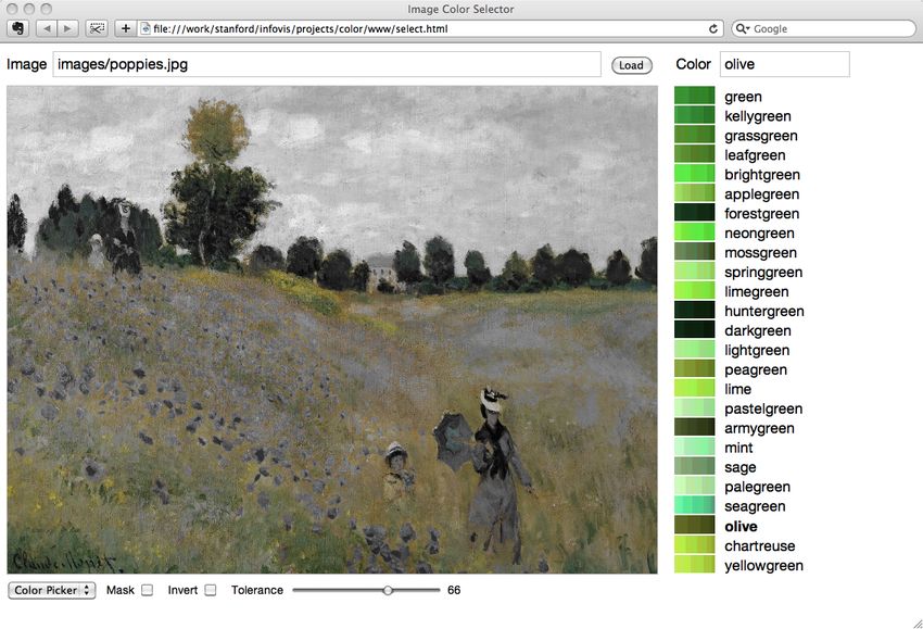
RELATED WORK                                                        ages. However, this approach requires that the color vocab-
Our research extends two streams of prior work: models of           ulary be known a priori, and provides little insight into the
color naming and user interfaces for color design.                  relative likelihood of color terms. Here, we seek to learn the
                                                                    kind and frequency of color terms used by people.
Models of Color Naming                                              In this paper, we build on the approach of Chuang et al. [8] to
Researchers have devised multiple approaches for modeling           construct a non-parametric probabilistic model of color nam-
human color naming, both to aid scientific understanding            ing. As we will describe, we modify their definition of color
and to improve applications such as gamut mapping [24] and          salience to improve comparability among colors and intro-
image analysis [20, 22]. One approach is to simply parti-           duce name-based color similarity measures. We demonstrate
tion color space, e.g., by uniform subdivision of hue in HLS        how to construct such models from a large, unconstrained set
color space [17]. Another is to create a color dictionary that      of color-name judgments. In particular, we use over 3 mil-
maps color names (basic color terms plus modifiers such as          lion color-name responses collected from readers of the web
“light”, “dark”, and “vivid”) to a single color value. This         comic XKCD. While prior work [22] has required that the
approach is used by the ISCC-NBS standard [15] and de-              desired number of color names be given as a model param-
rived variants [4, 11, 20]. These approaches map colors to          eter, we introduce a scaling routine that uses a measure of
names in a deterministic, disjoint fashion: they do not model       information loss to determine the number of color names.
association strength or overlap among color names.
                                                                    Tools for Color Design
Instead, color scientists use statistical models fitted to a cor-   Researchers in HCI, Computer Graphics, and Visualization
pus of human color-name judgments. Some researchers em-             have devised myriad tools and algorithms for assisting col-
ploy parametric models using a mixture of Gaussian [24,             orists. One prominent class of applications is interfaces for
26] or Gaussian-Sigmoid distributions [2]. While paramet-           color selection or palette design [1, 3, 12, 19, 28, 37]. For
ric models can suppress noise and be described with a small         example, PRAVDAColor [3] and ColorBrewer [12] suggest
set of parameters, they make assumptions about the shape of         color palettes for encoding data in visualizations based on
named color regions that may not match empirical distribu-          data types and/or cardinality. Meier et al. [19] apply theories
tions. For example, a Gaussian ellipsoid may assign proba-          of artistic color harmony [13, 18] to assist interactive color
bility mass to color values outside the gamut of interest.          selection. Cohen-Or et al. [9] use these same theories to for-
                                                                    mulate automated color harmonization methods for image
In response to these shortcomings, others have advocated
                                                                    composition. To our knowledge, none of these tools incor-
the use of non-parametric models that avoid assumptions re-
                                                                    porate nuanced models of color naming to aid color selection
garding the shape of color name distributions. Moroney [22]
                                                                    or image analysis. In this paper, we explore ways in which
models color naming using histograms over a binned color
                                                                    color naming models can augment color picking, pixel selec-
space. Chuang et al. [8] model color-name association using
                                                                    tion for image editing, and the evaluation of color palettes.
multinomial conditional probability distributions. Chuang
et al. also define a statistic for color salience — the unique-
ness of a color name — in terms of model entropy. Using the         CONSTRUCTING COLOR NAMING MODELS
330 colors of the World Color Survey [10], they find good           To construct a color naming model, we first process the in-
agreement among high salience scores and basic color name           put data: a collection of color-name pairs comprising nam-
“foci” identified in previous work [5, 35].                         ing judgments by human subjects. We present a method for
                                                                    reducing unconstrained text responses describing millions of
One issue affecting model construction is the size and gran-        unique colors into a compact table of color-name correspon-
ularity of training data. Early work uses results from con-         dences. We then construct a non-parametric probabilistic
trolled settings, often limited to a few hundred color stimuli      model of color naming that supports saliency and similarity
(e.g., [2]). More recent work (e.g., [8, 21, 25, 26]) employs       metrics based on color-name association.
web-based surveys to create larger corpora (though limited
to the sRGB gamut of computer monitors). While web-                 Data Collection
based surveys sacrifice the controlled display and lighting         We start with a color naming data set: a list of color-name
environment of a laboratory, they offer access to a greater         pairs provided by human subjects. Here a “color” (or “color
variety of people and display types. Researchers have noted         value”) is a stimulus shown to a respondent and a “color
consistent results when comparing such crowdsourced data            name” (or “color term”) is a text label provided by the re-
sets with data gathered under controlled conditions [21, 26].       spondent to describe that stimulus. Prior work has elicited
                                                                    naming judgments using physical color chips or calibrated
An alternative approach used in computer vision is to con-          monitors. Recent work [8, 21, 26] has applied crowdsourc-
struct probabilistic naming models in an automated fashion          ing on the web to collect color naming data and verified that
[30, 36]. Given color names as input, a system can query a          the results are consistent with those from controlled settings.
search engine for images associated with that color term; the
image pixels can be used to fit a statistical model of color-       In this paper, we use a publicly-accessible English-language
name association. This approach has the advantage of au-            color naming data set [25] compiled by Randall Munroe, the
tomated construction, and has led to better performance on          author of the popular web comic XKCD. The data was col-
classification and retrieval benchmarks for photographic im-        lected through a web survey advertised on the XKCD site.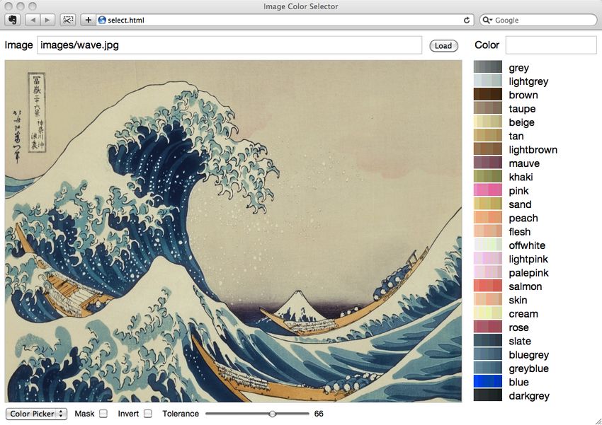
Respondents were asked to first provide basic demographic            space approximate color judgments made by human sub-
information: chromosomal sex, native language, color blind-          jects: a distance of 2.3 is roughly equal to one Just Notice-
ness, and optional information regarding monitor type, tem-          able Difference (JND) [31]. Measurements made within a
perature and gamma. Participants then named color swatches           local patch of L*a*b* space tend to correlate well with hu-
shown against a white background. Each color value was               man judgments; however, global measurements across the
expressed as a coordinate in sRGB color space; values were           color space can exhibit significant discrepancies. In response,
uniformly sampled from the full RGB cube. The text re-               color scientists have devised more sophisticated metrics for
sponses were unconstrained and respondents were free to              L*a*b* space that provide a closer fit to perceptual judg-
continue naming new swatches for as long as they wished.             ments. We use the current standard, CIEDE2000 [32], as
                                                                     our primary color distance metric.
The data set contains over 3.4 million responses from 152,401
sessions (103,430 self-reported males, 41,464 females, and           For the applications described in this paper, we construct
7,507 declined to state). To our knowledge this is the largest       color models using a bin size of 5 units within L*a*b* space.
color naming data set in existence. The top ten native lan-          Thus each bin has a radius of ∼1 JND and so subdivides
guages are English 74.6%, Not stated 12.2%, German 2.7%,             color space near the theoretical resolution of human color
Spanish 1.3%, French 1.2%, Dutch 1.1%, Swedish 0.8%,                 differentiation. Using 5-unit bins, the number of colors (ta-
Portuguese 0.6%, Polish 0.5%, and Russian 0.5%. The num-             ble rows) reduces from 2.3 million down to 8,325. For com-
ber of responses per participant ranges from 1 to 2,345 (me-         parison, using 10-unit bins results in 1,291 colors. To subse-
dian 18, inter-quartile range 10–30 responses). To combat            quently look up an input color in the table, we map it to its
malicious responses, the data set includes a per-user “spam          matching bin (interpolation methods could also be used).
score” that penalizes (a) responses that are not used by any-
one else and (b) the same response applied across high vari-
ations in hue. We keep only the responses from users with            Processing Color Terms
normalized spam scores ≤ 0.5. The spam-filtered data set             Unconstrained text responses result in a large and at times
consists of 3,252,134 color-name pairs spanning 2,956,183            amusing variety of color terms. While most responses use
unique RGB triples and 132,259 unique color names.                   common one or two word phrases (“blue”, “lavender”, “dark
                                                                     grey”, “hot pink”), there is a long tail of responses including
                                                                     rare (“butter yellow”) and bizarre (“velociraptor cloaca”) de-
The Color-Term Count Matrix                                          scriptions. Entity resolution is also a concern, as the same
The starting point for our model is a table (T ) of color-term       color name can have multiple variants (“blue green”, “blue-
counts in which rows represent colors, columns represent             green”, “blue/green”) and include misspellings (“fuchsia”
color terms, and each cell contains the count of responses           vs. “fuschia” & “fushia”). We would like to group variants
that use a color term to describe a corresponding color. Un-         representing the same color term, eliminate noise, and re-
surprisingly, a naïve tabulation yields a very sparse, high-         duce the dimensionality from 132,259 color terms to a more
dimensional matrix. In this section, we describe our method          manageable yet representative set.
for reducing the data to a compact and usable form. To limit
the number of colors (table rows), we bin color values within        To handle variants of punctuation and spacing, we first strip
a perceptual color space (CIE L*a*b*). To reduce the num-            all non-alphabetical characters (numbers, punctuation, white-
ber of terms (table columns), we apply a dimensionality re-          space, etc) from the response. This process maps many vari-
duction method. Finally, we smooth and filter the data.              ants to the same term (e.g., the previous blue-green examples
                                                                     map to “bluegreen”), removing about 20,000 variants and re-
Representing Color Values
                                                                     ducing the distinct term count to 114,860. We then tabulate
                                                                     a color-term count matrix T using the resulting terms.
To reduce the number of unique colors, we need to bin them
within a suitable color space. Uniform binning in sRGB is
                                                                     Next, we compute a lower-rank approximation of the color-
undesirable, as sRGB coordinates model color output de-
                                                                     term matrix to reduce dimensionality and remove noise. The
vices, not human perception: distances in sRGB space are
                                                                     idea is to remove the color terms (columns) that contribute
not generally consistent with perceptual judgments of color
                                                                     the least to the “information” contained within the data set.
difference. We want to group colors in a perceptually uni-
                                                                     We quantify this information
                                                                                               p using the Frobenius (element-
form fashion, preferably using a simple grid-based scheme.
                                                                     wise) matrix norm |T | = Σi,j (Tij )2 .
Accordingly, we bin colors within the standard CIE L*a*b*
color space using a D65 reference white point 1 . CIE L*a*b*         We first compute the sum of squares of each matrix column
is a 3-dimensional perceptual color space based on opponent          and sort the columns in ascending order. We then incremen-
process theory [27]. The L* dimension represents lightness           tally subtract these values from |T | to determine the matrix
and ranges from black (L*=0) to white (L*=100). The a*               norm |Tk | for the color-term count matrix with the k-lowest
and b* dimensions both range from roughly -100 to 100 and            columns removed. Given a threshold percentage value p, we
correspond to green-red and blue-yellow opponent channels,           can now find the maximal value of k such that |Tk |/|T | ≥ p.
respectively. Euclidean distances within CIE L*a*b* color            Retaining 99% of the information (p = 0.01) reduces the
                                                                     number of color terms to 66,526 – still a large a number.
1
  D65 is the standard reference white point used by sRGB, in which   The model used in this paper retains 95% of the information
the source color values are defined.                                 (p = 0.05), resulting in a reasonable set of 179 color names.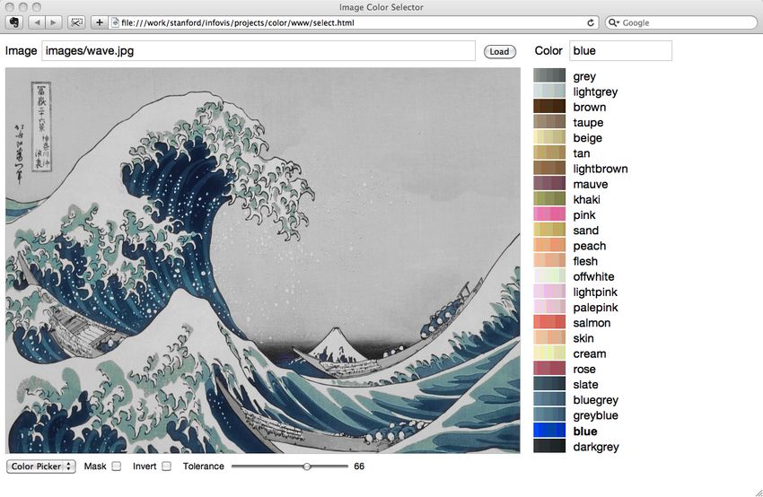
L* = 5                         L* = 15                        L* = 25                        L* = 35                        L* = 45

L* = 55                        L* = 65                        L* = 75                        L* = 85                        L* = 95

Figure 1. Color Saliency Map. Each point represents a 5×5×5 bin in CIE L*a*b* color space; slices for every other L* value are shown. The area
of each point is proportional to its saliency: large points indicate consistently named colors, small points indicate colors that exhibit high naming
confusion. Interestingly, visible clusters correspond to basic color terms identified by Berlin & Kay (blue, brown, green, grey, pink, purple, etc).

Our reduction technique optimizes the same metric as Sin-                     to compute additional metrics to analyze the effects of color
gular Value Decomposition (SVD), the method underlying                        naming. Here we describe our modeling approach and the
dimensionality reduction techniques such as Latent Seman-                     model-based metrics used in our subsequent applications.
tic Analysis (LSA). Whereas SVD finds a new set of basis
vectors to describe the data, our method simply zeroes-out                    Following Chuang et al. [8], we model the likelihoods of col-
the columns that make the smallest contribution to the matrix                 ors and names as multinomial probability distributions. We
norm, preserving each color term as a separate dimension.                     are concerned with the random variables C (which takes on
                                                                              color values) and W (which takes on color names). We use
While the above method successfully reduces color term di-                    the symbols c and w to denote specific values taken by these
mensionality, it does not handle misspellings. Fortunately,                   variables; the symbols also serve as indices for the rows (c)
the reduced color space is now small enough that manual                       and columns (w) of the color-term count matrix T .
correction takes only a few minutes. We add a hand-crafted
lookup table to the first stage of our processing pipeline to                 We can now express the likelihood of a color value given a
correct identified misspellings. We then re-tabulate T on the                 specific color name as the conditional probability p(C|w).
spell-corrected set of terms and perform dimensionality re-                   For each color c taken by C, we compute the probability by
duction again to produce a final set of 153 color names.                      normalizing the rows of T :
                                                                                                                X
                                                                                               p(c|w) = Tc,w /     Tc,w              (1)
Smoothing & Simplification
                                                                                                                        c
To arrive at our final table, we smooth the data and filter iso-
lated responses. To perform smoothing, we first represent                     Similarly, the probability p(W |c) of a name given a color is:
the color-term count matrix as a three-dimensional grid in                                                       X
                                                                                                p(w|c) = Tc,w /       Tc,w              (2)
L*a*b* space. We convolve the grid with a 3×3×3 kernel
                                                                                                                       w
with a value of 4 in the center and 1 in all other positions.
For each grid cell, we average over the adjacent non-zero                     These distributions give us the likelihood of a color condi-
grid cells weighted according to the kernel. We then round                    tioned on a specific term or vice versa. We can also model
the smoothed cell values to the nearest integer count. We                     the association between two colors or between two terms.
find that this approach adequately smooths the space with-                    Given a color c, the probability of other colors that have been
out over-blurring. Next, we zero-out any table cells with a                   labeled with matching names (the categorical association of
value of 1. We do this for two reasons: (1) if a color-term                   a color [8]) is given by
pair has only a single “vote”, there is no corroboration of                                             X
                                                                                               p(C|c) =      p(C|w)p(w|c)                 (3)
the judgment, and (2) dropping these cells significantly re-
                                                                                                             w
duces the size of the model with no discernible detriment in
subsequent applications.                                                      The categorical association between words p(W |w) is ex-
                                                                              pressed in a symmetric manner:
A Probabilistic Model of Color Names
                                                                                                        X
                                                                                             p(W |w) =      p(W |c)p(c|w)          (4)
Given a color-term count matrix, we can model the probabil-                                                    c
ity distributions of colors and names. We then use this model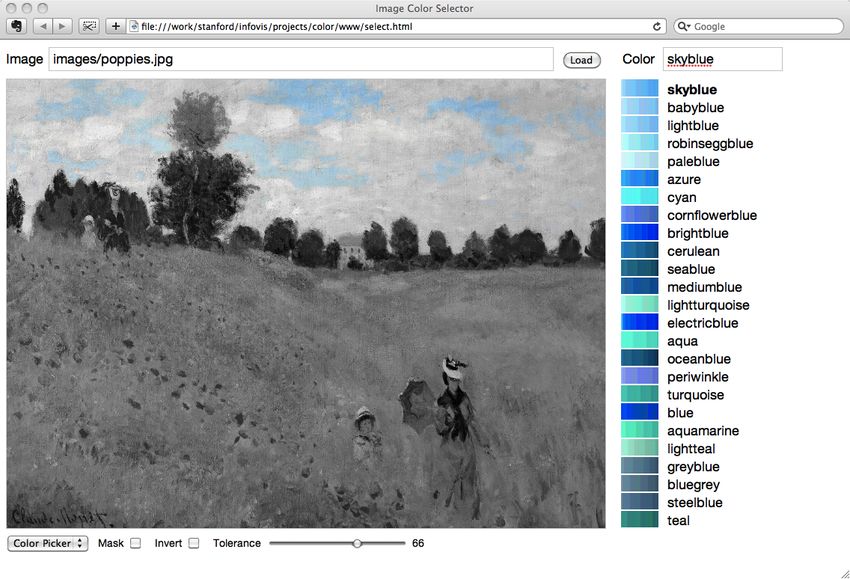
Color Saliency                                                    Name-Based Distance Measures
Given a probabilistic setting, we can use common measures         Our color naming model also enables new distance measures
to quantify other aspects of color naming. We define color        among color values. In addition to metrics within a color
saliency — the degree to which a color value is uniquely          space, we can compare two colors by how similarly they are
named — in terms of the entropy of the conditional probabil-      named. One option is to use a metric defined specifically for
ity p(W |c). Entropy (H) is a standard information-theoretic      probability distributions, such as the Hellinger distance:
measure of the “randomness” of a distribution. Specifically,                                  Xp
it measures the number of bits necessary to encode a random               Dh (a, b) = ( 1 −          p(w|a) p(w|b) )0.5      (6)
variable. If a color is uniquely named by all respondents,                                    w
there is no randomness and p(W |c) will have an entropy of        Though not grounded in probabilistic semantics, another op-
zero. For colors with a high degree of naming disagreement,       tion is to compute the cosine of the angle between two dis-
p(W |c) will have a correspondingly higher entropy. We thus       tributions. Due to normalization, this is equivalent to the co-
express saliency in terms of the negative entropy:                sine among rows of the color-term count matrix T . Denoting
                                   X                              the row vector of T for the color c as Tc , we have:
  Saliency(c) = −H(p(W |c)) =          p(w|c) log p(w|c) (5)
                                                                                                                Ta · Tb
                                       w                                Dc (a, b) = 1 − cos(Ta , Tb ) = 1 −                     (7)
                                                                                                              ||Ta || ||Tb ||
Figure 2 shows the distribution of saliency scores for the
XKCD data. To create a normalized saliency measure, we            Due to its simplicity and familiarity, we use the cosine metric
rescale the values from [-4.5, 0] to the interval [0,1].          to measure name-distance between two colors in our subse-
                                                                  quent applications. Using other metrics, such as Hellinger
                                                                  distance, produces qualitatively similar results.

                                                                  APPLICATIONS OF COLOR NAMING MODELS
                                                                  To demonstrate the utility of color naming models for graph-
                                                                  ical interfaces, we present a series of novel applications: a
                                                                  name-based color dictionary & thesaurus, name-based inter-
-4.5   -4    -3.5   -3    -2.5    -2       -1.5   -1   -0.5   0   action techniques for selecting image regions, and an evalua-
       Figure 2. Histogram of XKCD Color Salience Scores.
                                                                  tion tool for color palette design. The primary data structure
                                                                  used in each of these applications is the color-term count
                                                                  matrix T , from which we can compute probabilities, color
Our formulation of saliency differs from that of prior work.      salience, and color distance measures. We have implemented
Chuang et al. [8] define saliency as the negative entropy of      each example as a browser-based web application, written in
the distribution p(C|c), the categorical association between      JavaScript using the D3 (Data-Driven Documents) [6] frame-
colors. Using p(C|c) allows one to combine (often sparse)         work. Both the applications and our library of color model-
color naming data from multiple languages into a unified          ing routines is freely available as open-source software at:
“term-free” distribution. However, their formulation mea-         http://vis.stanford.edu/color-names.
sures the uniqueness of color names across the entire color
space, not at a single value. This occurs because the saliency    Color Dictionary & Thesaurus
values are biased by the volume of color space spanned by         A simple and direct application of color naming models is
a name. If one shade of blue and one shade of yellow are          to look up the color values associated with a name (a dictio-
both uniquely named (e.g., 100% of responders call color 1        nary) and find other, related color terms (a thesaurus). Fig-
“blue” and call color 2 “yellow”) the yellow shade will re-       ure 3 shows our interface for these tasks. Users might work
ceive a higher saliency value. This is because “yellow” oc-       with the interface to select colors (e.g., for graphic design)
cupies a smaller volume of color space and hence has higher       or explore relationships among color names.
p(C|w) values. To ensure saliency scores are comparable
across hues, we instead compute saliency using p(W |c).           In response to a color term query, the interface displays the
                                                                  most probable color values matching that color name. Next,
Figure 1 shows the distribution of saliency scores across         the thesaurus view lists related color names ranked by sim-
L*a*b* color space, clipped to the sRGB gamut. The saliency       ilarity. The top of the list shows highly similar color names
scores appear to cluster, with local maxima corresponding to      (synonyms), whereas the bottom (not shown) lists opposed
the basic color terms identified by Berlin & Kay. These clus-     color names (antonyms).
ters exhibit different shapes, lending credence to the use of
non-parametric models. We can also identify boundaries be-        Dictionary. Given a color name, retrieving representative
tween color names. Note the region of low saliency between        color values is straightforward: we find the most probable
green and blue. This area exhibits high naming confusion,         color values according to p(C|w). To select a single rep-
including the terms “teal”, “turquoise”, “green” and “blue.”      resentative color, we average the four most probable colors
Note also the narrow “valley” between orange and red at L*        (the four largest values of the p(C|w) distribution). We find
= 55. This fine-grained detail is visible due to the dense        that this produces more helpful results than choosing only
sampling of responses in the XKCD data; sparse data would         the single most probable value, particularly for names corre-
require larger bin sizes and hence lost detail.                   sponding to bright, desaturated colors.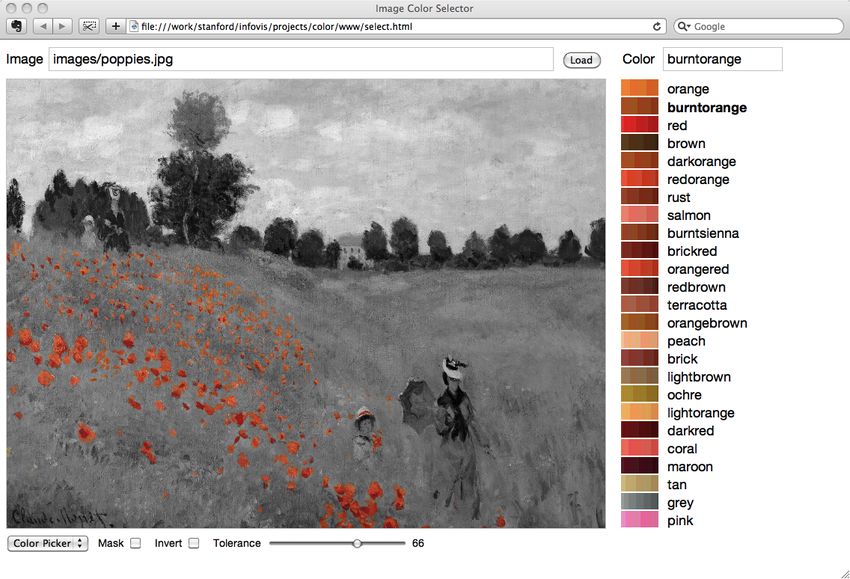
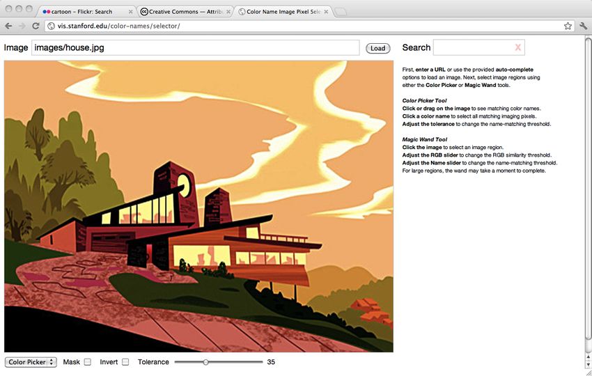
Color Name Queries
 Color mediumblue                                                        To select image pixels matching a color name w, we simply
                                                                         include those pixels with non-zero p(c|w) values. To control
                                                                         the sensitivity of the selection, users can adjust a tolerance
                                                                         parameter to set a minimum p(c|w) threshold. Users can
 #317cb2 #007fbb #3a6bad #0071ad                                         either type a color term query or interact with the image to
                                                                         generate relevant suggestions. In response to a mouse-driven
                                                                         selection, we show the most probable color names according
 #276cb6 #006fb6 #2b6abe #006dbe                                         to p(W |c). In the case of a single pixel, we use the corre-
                                                                         sponding probability distribution. In the case of image re-
                                                                         gions, we average the distributions for each pixel.
 #006fbe #006dc7 #0362a0 #00649f
                                                                         Figure 4 shows our image selection prototype. The left panel
                                                                         displays an image and the right panel shows a list of sug-
 #0a60a8 #0063a8 #0f5eb0 #0061b0                                         gested color names. By default, the list contains the most
                                                                         probable names for the entire image. The bottom panel in-
Similar Colors                                                           cludes a slider for adjusting selection tolerance (the p(c|w)
                                                                         threshold). Clicking a pixel or dragging over a rectangu-
                     cerulean                        #007ba9             lar region updates the list to show the most probable color
                                                                         names for those pixels. A user can page through each name-
                     cornflowerblue                  #7e8bf1             based selection using the up and down arrow keys. A user
                     oceanblue                       #006185             can also type in a search query, initiating a selection and re-
                                                                         vealing related color names based on our color thesaurus.
                     azure                           #4caaff
                     seablue                         #006f93             Figures 4–6 show the use of color name queries to isolate
                                                                         image regions of interest. Figure 5 shows selections result-
                     blueshowing the 16 most probable
Figure 3. Color dictionary                           #0032f7
                                                          color values   ing from a variety of color name queries, including the use of
for the query “mediumblue.” The thesaurus lists related color names      more specific, automatically suggested color names (“olive”,
                     brightblue
sorted according to p(query                          #004fff
                              | name). Ties are broken by sorting rep-   “forestgreen” and “puke”) to select sub-regions of an initial,
resentative colors by their CIEDE2000 distance.
                     electricblue                    #001ffd             general query (“green”). Figure 6 shows selections seeded
Thesaurus. To rank color names, we sort by the name-name                 by direct manipulation: the user can click a pixel or drag a
 Opposite
association     Colorsp(W |w). We score each color name
            probabilities                                                region to view related color names and then page through
by p(query | name), the probability of the query term given              the results to find a desired selection.
                  brightyellow
the name. Empirically,                           #f7f900
                           we have found that this  choice pro-
                  yellow
vides better results  than p(name | query), which#fff617
                                                      can priv-          A Name-Based Magic Wand Selector
ilege names with high marginal probability. For the query
term “mediumblue,”greenyellow                    #ccf90e
                        the name “purple” is ranked  highly ac-
                                                                         A common selection mechanism within image editors is the
                                                                         magic wand tool. Using the wand tool, a user first clicks a
cording to p(name lime| query)  because  it is a #bdff25
                                                 common
Choosing terms that instead maximize the likelihood of the
                                                          term.          desired pixel. The application then selects all adjacent pixels
                                                                         within a specified color distance using a flood-fill algorithm.
query favors similar   shades of blue (shown in #bdeb00
                  chartreuse                     Figure 3). The          Most wand tool implementations measure color distance as
sort order is determined by similarities in naming patterns,
which need not beyellowgreen                     #c6f335
                     the same as perceptual similarity  among
                                                                         the maximal absolute difference in the red, green, or blue
                                                                         channels – the L∞ norm in RGB space. A tolerance param-
                  limegreen
representative colors.                           #96f900to a
                         Again, a color name corresponds                 eter ranging from 0–255 controls the threshold distance.
variably sized distribution across a range of color values.
                    lightyellow                     #ffff91              Instead, we can use color naming distance — computed us-
To  break ties,Vertical
 Orientation:   we sort color names according to the percep-             ing the cosine of the angle between p(W |c) vectors — to de-
tual (CIEDE2000) distance between representative colors.                 termine pixel similarity. Our implementation provides a tol-
As some color names have association probabilities of zero               erance parameter with range 0–100, which maps to name-
(e.g., the hues yellow, orange, and red were never labeled               based distances on the interval [0, 1].
“blue”), sorting by perceptual distance ensures that color
antonyms align with opponent process theory: yellow is the               Figure 7 compares selections from an RGB-based wand and
antonym of blue, green is the antonym of red, and so on.                 a name-based wand. The name-based selection better re-
                                                                         spects color name boundaries and is more stable across a
Using Color Name Models for Image Editing                                range of tolerance settings. At low tolerance settings, RGB
People in conversation regularly use color names to refer to             distance fails to select a perceptually coherent brown region
visual elements. Color name models can enable analogous                  due to color value variation; at higher tolerances the selec-
forms of reference in user interfaces, for example, within               tion bleeds across color name boundaries, selecting adjacent
image editors such as Adobe Photoshop or Illustrator. Here               orange regions. In contrast, the color name wand selects the
we describe two techniques for name-based selection: color               brown region and excludes the orange pixels. To ensure that
name queries and a name-based magic wand selector.                       this discrepancy is not simply due to the use of RGB space,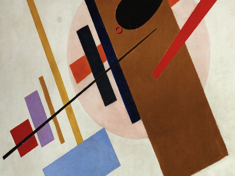
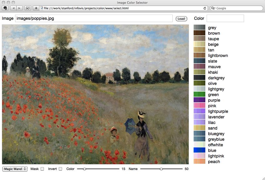
Blue, with non-selected pixels in grayscale

   The Great Wave off Kanagawa by Hokusai                                                            Blue, with non-selected pixels removed
Figure 4. Image selection by color name query. Left: Our prototype selection interface, listing the most probable color names according to p(W |c).
The many light colors correspond to the sky and boats. Beneath the image are selection options, including a tolerance parameter. Top-Right: The
selection for the color query “blue”, showing non-selected pixels in grayscale. Bottom-Right: The same query with non-selected pixels removed.

 From Flickr user “x-ray delta one”                 Red                                               Peach

 Olive                                              ForestGreen                                       Puke
Figure 5. Image regions selected by color name query. Non-selected pixels are shown in grayscale. The bottom row illustrates selections made when
moving from a basic color term (“green”) to more specific terms to isolate foliage (“olive”), dark grass (“forestgreen”) or tree tops (“puke”).

 Poppies, Near Argenteuil by Monet    BurntOrange                           SkyBlue                               Olive
Figure 6. Image regions selected by color name query. Non-selected pixels are shown in grayscale. The selected query terms were chosen from a list
of most probable colors for an image region selected by mouse-drag. In this case, a user can rapidly isolate flower, sky, and foliage pixels.
tRGB = 30               tRGB = 60               tRGB = 60 (zoom-in)

 Suprematism (Supremus No. 58) by Malevich
 The red circle indicates the input pixel to the magic wand.
                                                                            tNames = 10             tNames = 40             tNames = 40 (zoom-in)
Figure 7. Magic wand pixel selections based on RGB distance (top row) and color name similarity (bottom row) across a range of parameter values.
The RGB selector misses pixels at low tolerance values (t=30) and includes orange and red hues at higher tolerance values (t=60). The color name
selector produces more uniform results across parameter settings and is sensitive to color name boundaries.

we also implemented a magic wand based on CIEDE2000                        among colors, while bar charts show salience scores. These
distance in L*a*b* space. We observed qualitatively simi-                  metrics enable rapid comparison of the palettes. Tableau
lar results as the RGB-based selector: low tolerances lead to              and ColorBrewer both limit name overlap and include high-
under-selection and higher tolerances lead to color “bleed.”               salience colors. The Excel and Economist palettes, on the
                                                                           other hand, exhibit high naming overlap and lower salience
Of course, not all name-based selections work so perfectly.                colors. A designer can use these displays to evaluate differ-
We observe that desaturated colors (e.g., pastels) have higher             ent color choices and assess questions such as: “If I shift the
name overlap, leading to less granular selections. Excluding               cyan more towards green, will it change names?”
achromatic names (e.g., “grey”) may improve the situation.
In addition, we have combined color space and name-based                   Figure 9 shows diverging palettes for numerical data with
distances within a hybrid wand tool that selects either the                a meaningful mid-point. The first palette, used in the Map
union or intersection of the two selection measures. This                  of the Market [38], naïvely ramps from red through black
hybrid tool uses two tolerance parameters (one for names,                  to green in RGB space. The other three palettes come from
one for color space) and enables more nuanced selections.                  ColorBrewer. We note that the Map of the Market palette
                                                                           has significant name overlap on each ramp, while the Col-
Evaluating Color Palette Designs                                           orBrewer palettes show more naming variation. In displays
Color design experts [7, 34, 33] argue that attention to color             such as choropleth maps, simultaneous contrast can ham-
names is important in palette design, particularly for infor-              per subtle luminance comparisons [34]. By including small
mation visualization. First, nameable colors facilitate com-               shifts in color hue and naming, the ColorBrewer palettes
munication: it is easier to refer to graphical elements when               may improve discrimination. Yet by making the shifts sub-
one can name them unambiguously. Second, experimental                      tle, the colors are still perceived as a ramp. ColorBrewer
evidence suggests that highly nameable colors are better re-               palettes also exhibit salience gradients oriented toward ex-
membered [29], perhaps due to the cue of the color name.                   treme values, emphasizing greater deviation from the mid-
To inform color palette design, we use our model to quan-                  point through both luminance and categorical salience.
titatively characterize palettes with respect to color naming.
To analyze a color palette, we examine both individual color               While informative for human designers, these metrics might
saliency scores and color name distances. This data can help               also improve automated design tools, for example by mini-
designers reason about the effects of color choices.                       mizing name overlap and increasing saliency. Of course, ef-
                                                                           fective color design involves many concerns, including other
To optimize the presentation of categorical data, we might                 contrast effects and cultural associations. In future work, we
seek to minimize name overlap (to avoid ambiguity) and                     plan to apply our naming model to automatically optimize
maximize salience (to avoid confusion and aid memory).                     color palette design and evaluate the results.
Figure 8 characterizes qualitative color palettes for encoding
categorical data. The palettes come from Tableau (a visual-                DISCUSSION
ization tool with palettes designed by a color specialist [33]),           In this paper, we presented a method of constructing a prob-
the ColorBrewer selection tool [12], Microsoft Excel, and                  abilistic model of color naming from large, unconstrained
The Economist magazine. Tables show color name distances                   naming data sets. We described a model based on over 3 mil-
palettes r_rainbow r_grays economist tableau10 tableau20 excel10 manyeyes brewer_q09 brewer_q10
palettes
brewer_q12
r_rainbowbrewer_da
r_grays economist
brewer_db tableau10
brewer_dctableau20
brewer_ddexcel10
marketmap
manyeyes brewer_q09 brewer_q10 brewer_q
Color Name Distance Salience Name Color Name Distance Salience Name
0.00 1.00 1.00 1.00 0.96 1.00 1.00 0.99 1.00 .47 blue 65.3%
0.19 0.00 0.42 1.00 1.00 1.00 1.00 1.00 1.00 0.92 0.97 .31 lightblue 30.4%
1.00 0.00 1.00 0.98 1.00 1.00 1.00 1.00 0.97 .87 orange 92.2%
1.00 0.42 0.00 1.00 1.00 1.00 1.00 1.00 1.00 0.95 0.94 .47 blue 65.3%
1.00 1.00 0.00 1.00 1.00 1.00 1.00 1.00 0.70 .70 green 81.3%
0.99 1.00 1.00 0.00 0.33 1.00 1.00 0.99 1.00 1.00 1.00 .28 green 26.9%
1.00 0.98 1.00 0.00 1.00 0.96 0.99 1.00 1.00 .64 red 79.3%
1.00 1.00 1.00 0.33 0.00 1.00 1.00 1.00 1.00 1.00 1.00 .70 green 81.3%
0.96 1.00 1.00 1.00 0.00 0.95 0.83 0.98 1.00 .43 purple 52.5%
0.97 1.00 1.00 1.00 1.00 0.00 0.97 0.90 1.00 0.84 1.00 .49 pink 54.1%
1.00 1.00 1.00 0.96 0.95 0.00 0.99 0.96 0.96 .47 brown 60.5%
1.00 1.00 1.00 1.00 1.00 0.97 0.00 0.96 0.93 1.00 1.00 .69 red 79.0%
1.00 1.00 1.00 0.99 0.83 0.99 0.00 1.00 1.00 .47 pink 60.3%
1.00 1.00 1.00 0.99 1.00 0.90 0.96 0.00 0.44 1.00 1.00 .28 peach 25.0%
0.99 1.00 1.00 1.00 0.98 0.96 1.00 0.00 1.00 grey
0.99
.74 83.7% 1.00 1.00 1.00 1.00 1.00 0.93 0.44 0.00 1.00 1.00 .89 orange 93.3%
1.00 0.97 0.70 1.00 1.00 0.96 1.00 1.00 0.00 .11 yellow 20.1%
1.00 0.92 0.95 1.00 1.00 0.84 1.00 1.00 1.00 0.00 0.61 .22 lavender 23.6%
0.19 1.00 0.99 1.00 0.97 1.00 1.00 0.99 1.00 0.00
.25 blue 27.2% 0.97 0.94 1.00 1.00 1.00 1.00 1.00 1.00 0.61 0.00 .53 purple 67.3%
Tableau-10 Average 0.96 .52 ColorBrewer-Q10 Average 0.94 .49
palettes r_rainbow r_grays economist tableau10 tableau20 excel10 manyeyes brewer_q09 brewer_q10
palettes
brewer_q12
r_rainbowbrewer_da
r_grays economist
brewer_db tableau10
brewer_dctableau20
brewer_ddexcel10
marketmap
manyeyes brewer_q09 brewer_q10 brewer_q
Color Name Distance Salience Name Color Name Distance Salience Name
0.00 1.00 1.00 0.89 0.08 1.00 0.19 1.00 1.00 0.88 .44 blue 61.5% 0.00 0.97 1.00 1.00 1.00 1.00 1.00 0.99 .32 brown 37.4%
1.00 0.00 0.99 1.00 1.00 0.81 1.00 0.78 1.00 0.99 .21 red 21.1% 0.97 0.00 1.00 1.00 1.00 1.00 1.00 1.00 .29 pink 24.5%
1.00 0.99 0.00 1.00 0.98 0.99 1.00 1.00 0.10 1.00 .39 green 42.8% 1.00 1.00 0.00 0.37 0.20 0.38 0.82 0.99 .43 blue 57.1%
0.89 1.00 1.00 0.00 0.92 1.00 0.80 0.84 1.00 0.31 .42 purple 57.8% 1.00 1.00 0.37 0.00 0.59 0.53 0.77 0.95 .23 blue 24.6%
0.08 1.00 0.98 0.92 0.00 1.00 0.21 1.00 0.97 0.88 .24 blue 40.4% 1.00 1.00 0.20 0.59 0.00 0.44 0.85 0.99 .36 blue 27.3%
1.00 0.81 0.99 1.00 1.00 0.00 1.00 0.92 1.00 1.00 .28 orange 36.3% 1.00 1.00 0.38 0.53 0.44 0.00 0.19 0.96 .14 teal 24.0%
0.19 1.00 1.00 0.80 0.21 1.00 0.00 0.94 0.97 0.58 .16 blue 25.6% 1.00 1.00 0.82 0.77 0.85 0.19 0.00 0.97 .22 teal 30.1%
1.00 0.78 1.00 0.84 1.00 0.92 0.94 0.00 0.99 0.76 .10 pink 21.8% 0.99 1.00 0.99 0.95 0.99 0.96 0.97 0.00 .68 grey 80.6%
1.00 1.00 0.10 1.00 0.97 1.00 0.97 0.99 0.00 0.96 .21 green 30.8% The Economist Average 0.82 .33
0.88 0.99 1.00 0.31 0.88 1.00 0.58 0.76 0.96 0.00 .25 purple 22.7%
Excel-10 Average 0.86 .27
Figure 8. Name-based characterization of qualitative color palettes. Matrices show all pairwise color-name distances; bar charts show salience scores
for each color. Salience scores below 0.2 indicate colors with a high degree of naming confusion. The Tableau-10 palette provides the best color
salience and minimal name overlap. Palettes from Excel and The Economist exhibit higher name overlap and diminished saliency.
palettes r_rainbow r_grays economist tableau10 tableau20 excel10 manyeyes brewer_q09 brewer_q10
palettes
brewer_q12
r_rainbowbrewer_da
r_grays economist
brewer_db tableau10
brewer_dctableau20
brewer_ddexcel10
marketmap
manyeyes brewer_q09 brewer_q10 brewer_q
Color Name Distance Salience Name Color Name Distance Salience Name
0.00 0.01 0.76 1.00 1.00 1.00 1.00 .79 red 85.3% 0.00 0.74 0.96 1.00 1.00 1.00 1.00 .70 brown 80.5%
0.01 0.00 0.68 1.00 1.00 1.00 1.00 .57 red 70.1% 0.74 0.00 0.28 0.98 1.00 1.00 1.00 .23 tan 31.7%
0.76 0.68 0.00 0.94 1.00 1.00 1.00 .25 maroon 26.3% 0.96 0.28 0.00 0.68 0.87 1.00 0.99 .17 beige 24.8%
1.00 1.00 0.94 0.00 0.98 1.00 1.00 .84 black 90.3% 1.00 0.98 0.68 0.00 0.40 0.90 0.96 .24 white 22.6%
1.00 1.00 1.00 0.98 0.00 0.20 0.35 .54 green 43.3% 1.00 1.00 0.87 0.40 0.00 0.54 0.83 .11 lightblue 20.1%
1.00 1.00 1.00 1.00 0.20 0.00 0.15 .71 green 81.6% 1.00 1.00 1.00 0.90 0.54 0.00 0.19 .16 teal 21.4%
1.00 1.00 1.00 1.00 0.35 0.15 0.00 .46 green 41.2% 1.00 1.00 0.99 0.96 0.83 0.19 0.00 .17 teal 27.2%
Map of the Market Average 0.81 .59 ColorBrewer-Div1 Average 0.82 .26
palettes r_rainbow r_grays economist tableau10 tableau20 excel10 manyeyes brewer_q09 brewer_q10
palettes
brewer_q12
r_rainbowbrewer_da
r_grays economist
brewer_db tableau10
brewer_dctableau20
brewer_ddexcel10
marketmap
manyeyes brewer_q09 brewer_q10 brewer_q
Color Name Distance Salience Name Color Name Distance Salience Name
0.00 0.96 0.96 0.99 1.00 1.00 1.00 .41 red 57.7% 0.00 0.43 0.86 1.00 1.00 1.00 1.00 .62 purple 72.0%
0.96 0.00 0.52 0.99 1.00 1.00 1.00 .30 peach 25.9% 0.43 0.00 0.45 0.94 0.98 1.00 1.00 .35 lavender 25.8%
0.96 0.52 0.00 0.79 0.98 1.00 1.00 .22 pink 21.7% 0.86 0.45 0.00 0.45 0.69 1.00 1.00 .17 pink 16.4%
0.99 0.99 0.79 0.00 0.56 0.83 0.92 .24 white 22.6% 1.00 0.94 0.45 0.00 0.44 1.00 1.00 .24 white 22.6%
1.00 1.00 0.98 0.56 0.00 0.25 0.67 .27 lightblue 27.8% 1.00 0.98 0.69 0.44 0.00 0.54 0.71 .02 grey 10.9%
1.00 1.00 1.00 0.83 0.25 0.00 0.16 .32 blue 37.3% 1.00 1.00 1.00 1.00 0.54 0.00 0.09 .35 green 49.8%
1.00 1.00 1.00 0.92 0.67 0.16 0.00 .60 blue 75.1% 1.00 1.00 1.00 1.00 0.71 0.09 0.00 .59 green 61.4%
ColorBrewer-Div2 Average 0.84 .34 ColorBrewer-Div3 Average 0.79 .33
Figure 9. Name-based characterization of diverging quantitative color palettes. Naïve interpolation in RGB space (as in the Map of the Market) leads
to name overlap among non-adjacent colors. ColorBrewer palettes (excluding “teal”) exhibit salience gradients towards the extreme values.
lion web survey responses — to our knowledge the largest pies a larger volume. Future large-scale surveys might vary
color naming data set in existence — and showed how it can the background color among black, white, and one or more
be used to map between colors and names, calculate color shades of grey to construct color naming models more sensi-
saliency, and measure color similarity based on naming pat- tive to background contrast. Alternatively, automated meth-
terns. We then introduced a set of novel applications that ods (e.g., using image search engines [30, 36]) might be used
illustrate how color naming models can enhance graphical to refine color name regions.
user interfaces: a color dictionary & thesaurus, name-based
pixel selection techniques for image editing, and evaluation While our approach uses CIE L*a*b* color space, recent
aids for comparing color palette designs. Through these ex- work in color science concerns color appearance models.
amples, we demonstrate that color naming models enable These models incorporate contrast effects due to background
users to express their intentions in new ways and offer de- and surround regions. Though unable to predict all the intri-
signers new avenues for assessing their designs. cate effects of human color vision, a color appearance model
such as CIECAM02 [23] might associate colors with names
Though our initial results are encouraging, some limitations while taking contrast into account. Future research is needed
remain. All respondents in the XKCD survey were asked to assess the potential benefits and determine if the addi-
to name colors shown against a white background, a design tional modeling complexity is warranted.
decision that biases the results. Unsurprisingly, the region
of color space named “white” is small, as respondents were Our current work uses an English-language color naming
presumably sensitive to background contrast for high lumi- data set. In subsequent work we would like to construct color
nance colors, naming nearby colors “offwhite”, “cream”, or naming models across a variety of languages (c.f., [26]).
“light grey.” The term “black,” on the other hand, occu- Multi-lingual color naming data can enable scientific inves-
tigation of linguistic differences in color naming, for ex-                12. M. Harrower and C. Brewer. Colorbrewer.org: an online tool for
ample to verify basic color terms and assess differences in                    selecting colour schemes for maps. The Cartographic Journal,
color name boundaries and saliencies. Cross-language mod-                      40(1):27–37, 2003.
els would support internationalization of color name-based                 13. J. Itten. The Art of Color. Van Nostrand Reinhold Company, 1960.
applications and could potentially lead to culturally sensitive            14. P. Kay and C. K. McDaniel. The linguistic significance of the
                                                                               meanings of basic color terms. Language, 54(3):610–646, 1978.
color transfer or gamut mapping methods.
                                                                           15. K. L. Kelly and D. B. Judd. Color, universal language and dictionary
                                                                               of names. National Bureau of Standards (U.S.) Publ. 440, 1976.
We developed our applications through a design exploration                 16. G. Lakoff. Women, Fire, and Dangerous Things. University Of
of how color naming models might significantly enhance                         Chicago Press, 1990.
user interfaces. The goal of this process was to establish the             17. Y. Liu, D. Zhang, G. Lu, and W.-Y. Ma. Region-based image retrieval
utility of color naming models and develop new techniques.                     with high-level semantic color names. In Proc. IEEE International
We believe that each application provides novel support for                    Multimedia Modeling Conference, pages 180–187, 2005.
real-world tasks and initial feedback from informal usage                  18. Y. Matsuda. Color Design. Asakura Shoten, 1995.
has been positive. Users have expressed appreciation for the               19. B. Meier, A. Spalter, and D. Karelitz. Interactive color palette tools.
applications (including requests for the software) and have                    IEEE Comp. Graphics & App., 24(3):64–72, 2004.
suggested interesting use cases. For example, one person                   20. A. Mojsilovic. A computational model for color naming and
                                                                               describing color composition of images. IEEE Trans. Image
used name-based pixel selection to analyze a series of art                     Processing, 14(5):690–699, 2005.
works and “deconstruct” the coloring choices of the artist.                21. N. Moroney. Unconstrained web-based color naming experiment. In
                                                                               Proc. SPIE Color Imaging: Device-Dependent Color, Color Hardcopy
However, we do not claim that these applications are “fin-                     and Graphic Arts VIII, 2003.
ished.” Further design iteration and end-user evaluation will              22. N. Moroney. US Patent Application 11/259,597: Adapative lexical
undoubtedly refine these applications and inform how they                      classification system, 2007.
could be incorporated into existing tools and workflows. To                23. N. Moroney, M. Fairchild, R. Hunt, C. Li, M. R. Luo, and T. Newman.
facilitate future work, our color naming model and applica-                    The CIECAM02 color appearance model. In Color Imaging
                                                                               Conference, pages 23–27, 2002.
tions are available as open-source software, downloadable
                                                                           24. H. Motomura. Categorical color mapping using color-categorical
from http://vis.stanford.edu/color-names.                                      weighting method. Part I: Theory. J. of Imaging Science and
                                                                               Technology, 45(2):117–129, 2001.
ACKNOWLEDGEMENTS                                                           25. R. Munroe. Color survey results. http://blog.xkcd.com/
The authors thank Randall Munroe of XKCD for sharing his                       2010/05/03/color-survey-results/, May 2010.
color survey data, and Jason Chuang and Pat Hanrahan for                   26. D. Mylonas, L. MacDonald, and S. Wuerger. Towards an online color
their helpful insights and conversation. This work was sup-                    naming model. In Color Imaging Conference, pages 140–144, 2010.
ported by NSF Grant IIS-1017745.                                           27. S. Palmer. Vision Science: Photons to Phenomenology. MIT Press,
                                                                               1999.
                                                                           28. P. Rheingans and B. Tebbs. A tool for dynamic explorations of color
REFERENCES                                                                     mappings. ACM SIGGRAPH Comp. Graphics, 24(2):145–146, 1990.
 1. Adobe Kuler. http://kuler.adobe.com/.
                                                                           29. D. Roberson, D. I., and J. Davidoff. Colour categories are not
 2. R. Benavente, F. Tous, R. Baldrich, and M. Vanrell. Statistical            universal: Replications and new evidence from a stone-age culture.
    modelling of a colour naming space. In European Conference on              Journal of Experimental Psychology: General, 129:369–398, 2000.
    Colour Graphics, Imaging, and Vision, pages 406–411, 2002.             30. B. Schauerte and G. A. Fink. Web-based learning of naturalized color
 3. L. D. Bergman, B. E. Rogowitz, and L. A. Treinish. A rule-based tool       models for human-machine interaction. In Proceedings of the 2010
    for assisting colormap selection. In Proc. IEEE Visualization, pages       International Conference on Digital Image Computing: Techniques
    118–125, 1995.                                                             and Applications, pages 498–503, 2010.
 4. T. Berk, L. Brownston, and A. Kaufman. A new color-naming system       31. G. Sharma. Digital Color Imaging Handbook. CRC Press, 2002.
    for graphics languages. IEEE Comp. Graphics & App., 2(3), 1982.        32. G. Sharma, W. Wu, and E. N. Dalal. The CIEDE2000 color-difference
 5. B. Berlin and P. Kay. Basic Color Terms: Their Universality and            formula: Implementation notes, supplementary test data, and
    Evolution. Univ. of California Press, 1969.                                mathematical observations. Color Research & Applications,
                                                                               30(1):21–30, 2005.
 6. M. Bostock, V. Ogievetsky, and J. Heer. D3: Data-driven documents.
                                                                           33. M. Stone. Color in information display.
    IEEE Trans. Visualization & Comp. Graphics, 17(12):2301–2309,
                                                                               http://www.stonesc.com/VisCourses.htm.
    2011.
                                                                           34. M. Stone. A Field Guide to Digital Color. A. K. Peters, 2003.
 7. C. Brewer. Color use guidelines for data representation. In Proc.
                                                                           35. J. Sturges and T. W. A. Whitfield. Locating basic colours in the
    Section on Statistical Graphics, American Statistical Association,
                                                                               Munsell space. Color Research & Applications, 20(5):364–376, 1995.
    pages 55–60, 1999.
                                                                           36. J. van de Weijer, C. Schmid, J. Verbeek, and D. Larlus. Learning color
 8. J. Chuang, M. Stone, and P. Hanrahan. A probabilistic model of the         names for real-world applications. IEEE Trans. Image Processing,
    categorical association between colors. In Color Imaging Conference,       18(7):1512–1523, July 2009.
    pages 6–11, 2008.
                                                                           37. L. Wang, J. Giesen, K. McDonnell, P. Zolliker, and K. Mueller. Color
 9. D. Cohen-Or, O. Sorkine, R. Gal, T. Leyvand, and Y.-Q. Xu. Color           design for illustrative visualization. IEEE Trans. Visualization &
    harmonization. In ACM SIGGRAPH, pages 624–630, 2006.                       Comp. Graphics, 14(6):1739–1754, Nov-Dec 2008.
10. R. Cook, P. Kay, and T. Regier. The World Color Survey database:       38. M. Wattenberg. Visualizing the stock market. In Extended Abstracts,
    history and use. Elsevier, 2005.                                           ACM Human Factors in Computing Systems (CHI), 1999.
11. M. Das, R. Manmatha, and E. M. Riseman. Indexing flowers by color      39. J. Winawer, N. Witthoft, M. Frank, L. Wu, A. Wade, and
    names using domain knowledge-driven segmentation. In Proc. IEEE            L. Boroditsky. Russian blues reveal effects of language on color
    Workshop on Applications of Computer Vision (WACV’98), pages               discrimination. Proceedings of the National Academy of Sciences,
    94–99, 1998.                                                               104(19):7780–7785, 2007.
You can also read