Computational Methods for Predicting Protein-Protein Interactions Using Various Protein Features - Daisuke Kihara
←
→
Page content transcription
If your browser does not render page correctly, please read the page content below
Computational Methods for Predicting
Protein-Protein Interactions Using
Various Protein Features
Ziyun Ding1 and Daisuke Kihara1,2,3
    1
      Department of Biological Science, Purdue University, West Lafayette, Indiana
    2
      Department of Computer Science, Purdue University, West Lafayette, Indiana
    3
      Corresponding author: dkihara@purdue.edu

        Understanding protein-protein interactions (PPIs) in a cell is essential for learn-
        ing protein functions, pathways, and mechanism of diseases. PPIs are also im-
        portant targets for developing drugs. Experimental methods, both small-scale
        and large-scale, have identified PPIs in several model organisms. However,
        results cover only a part of PPIs of organisms; moreover, there are many organ-
        isms whose PPIs have not yet been investigated. To complement experimental
        methods, many computational methods have been developed that predict PPIs
        from various characteristics of proteins. Here we provide an overview of lit-
        erature reports to classify computational PPI prediction methods that consider
        different features of proteins, including protein sequence, genomes, protein
        structure, function, PPI network topology, and those which integrate multiple
        methods.  C 2018 by John Wiley & Sons, Inc.

        Keywords: computational methods r bioinformatics r protein-protein interac-
        tions, PPI r protein docking r protein interaction network

                                 How to cite this article:
               Ding, Z., & Kihara, D. (2018). Computational methods for
               predicting protein-protein interactions using various protein
                 features. Current Protocols in Protein Science, e62. doi:
                                     10.1002/cpps.62

INTRODUCTION
Identification of protein-protein interactions (PPIs) is important for understanding how
proteins work together in a coordinated fashion in a cell to perform cellular functions.
PPIs are essential for protein function, various cellular pathways, and development of
diseases. PPIs are also important targets for drug design. Understanding how proteins
interact can also lead to artificial design of protein interactions.

Individual PPIs are determined by experiments, such as co-immunoprecipitation
(A. Guo et al., 2005), fluorescence resonance energy transfer (Kenworthy, 2001), and
surface plasmon resonance (Nikolovska-Coleska, 2015). Ultimately, biophysical meth-
ods, such as nuclear magnetic resonance spectroscopy (NMR; Vinogradova & Qin, 2011;
Zuiderweg, 2002), X-ray crystallography (Kobe et al., 2008), and electron microscopy
(Dudkina, Kouřil, Bultema, & Boekema, 2010), solve the tertiary structure of protein
complexes, which can provide detailed atomic information about how the proteins in-
teract. Moreover, from the mid 1990’s, PPIs were determined on a large-scale using
the yeast-two-hybrid system (Fields & Sternglanz, 1994; Rajagopala et al., 2014; Rual
et al., 2005; Walhout, Boulton, & Vidal, 2000), and affinity chromatography combined
with mass spectrometry (Boeri Erba & Petosa, 2015; Dunham, Mullin, & Gingras, 2012;

                                                                                              Ding and Kihara

            Current Protocols in Protein Science e62                                          1 of 27
            Published in Wiley Online Library (wileyonlinelibrary.com).
            doi: 10.1002/cpps.62

            C 2018 John Wiley & Sons, Inc.
Guruharsha et al., 2011; Morris et al., 2014). However, experimental methods have several
shortcomings for detecting PPIs. First, these experimental methods are time consuming
and labor intensive. Second, the applicability of experimental methods depends on how
effectively assay protocols are established in target organisms. Also, a method may not
work on some classes of proteins (Piehler, 2005; Rao, Srinivas, Sujini, & Kumar, 2014).
Third, it is known that experimental methods often have difficulty with identifying weak
interactions, and leave out many transient interactions (Wetie et al., 2013). Fourth, it has
been mentioned that results of large-scale methods often have substantial disagreement
with each other, which may be partly due to false positives and false negatives (Gingras,
Gstaiger, Raught, & Aebersold, 2007; Huang & Bader, 2009; Serebriiskii & Golemis,
2001).
In Table 1, databases of PPIs are listed. Most of the identified PPIs are from model organ-
isms such as Escherichia coli, Homo sapiens, Mus musculus, Saccharomyces cerevisiae
(baker’s yeast), Schizosaccharomyces pombe (fission yeast), Drosophila melanogaster,
and Arabidopsis thaliana. Although large efforts have been made for detecting PPIs,
there still exists a huge gap between the experimentally identified PPIs and actual PPIs.
For example, it was estimated that humans have over 650,000 PPIs based on a statistical
method that evaluates the number of undiscovered PPIs from the known human PPI net-
work (Stumpf et al., 2008), whereas a little over 40,000 interactions have been identified
based on the Human Protein Reference Database (HPRD; Prasad et al., 2009). Even for
yeast, which is one of the most well studied organisms in terms of PPIs, 91,551 were iden-
tified based on the BioGrid database (Chatr-Aryamontri et al., 2017), whereas 240,000
PPIs were estimated. For Caenorhabditis elegans, which is an important model organ-
ism, only 5,797 PPIs were identified among 220,000 estimated. Thus, currently identified
PPIs derived from experiments only cover a small fraction in the entire PPI networks.
Hence, there is a strong need for computational methods for predicting PPIs, and indeed
many computational approaches have been developed to facilitate investigation of PPI
networks in organisms.
Computational PPI prediction methods were reviewed in several earlier articles. Com-
parative genomics-based methods were reviewed in 2002; shortly after a couple of
large-scale PPI networks emerged (Valencia & Pazos, 2002). Skrabanek et al. reviewed
methods that use comparative genomics and gene expression data, as well as tools for
visualizing PPIs (Skrabanek, Saini, Bader, & Enright, 2008). A review by Browne et al.
focused on experimental methods for PPI detection and classified existing methods based
on underlined machine learning algorithms (Browne, Zheng, Wang, & Azuaje, 2010).
A review by Liu et al. discussed computational methods by classifying them into two
groups, those which directly map information of known PPIs onto unknown protein pairs,
and approaches that employ machine learning methods to classify protein pairs from a
dataset of known PPIs and non-PPIs (Liu & Chen, 2012). Very recently, Chang et al.
focused on methods that combine different types of evidence for predicting PPIs (Chang,
Zhou, Ul Qamar, Chen, & Ding, 2016).
The current article classifies and reviews computational PPI prediction methods by
features of proteins considered for prediction, which includes protein sequence-based,
comparative genomics-based, gene expression-based, function-based, structure-based,
and network-based prediction methods. This article has some overlaps in its scope with the
previous review articles, but it is distinct from others by providing extensive discussion on
protein sequence-based prediction methods and network-based prediction methods, and
of course, by providing up-to-date information in this field. We also discuss applicability
of each type of methods in genome-scale PPI predictions.
Ding and Kihara
2 of 27
Current Protocols in Protein ScienceTable 1 List of Available Protein-Protein Interaction Databasesa
Database # of interactions Description Organisms Website Last update
BioGrid 1,110,310 Manually curated PPIs 62 https://thebiogrid.org/ Mar 2017
STRING 932,553,897 Protein associations including 2,031 https://string-db.org/ Jan 2017
PPIs
Current Protocols in Protein Science
DIP 81,731 Experimentally identified PPIs 834 https://dip.doe-mbi.ucla.edu/dip/Main.cgi Mar 2017
CORUM 6,375 Manually curated protein 10 https://mips.helmholtz-muenchen.de/corum/ Dec 2016
complexes in mammals
IntAct 718,180 PPIs taken from literature and Model organisms including https://www.ebi.ac.uk/intact/ Mar 2017
from user submissions human, mouse, yeast, fruitfly, C.
elegans, E. coli, A. thaliana
MINT 125,464 Experimentally verified PPIs 611 https://mint.bio.uniroma2.it/ Mar 2017
from literature
InnateDB 367,478 Manually curated PPIs for Human, mouse, B. taurus https://www.innatedb.com/ Nov 2016
mammalian innate immune
response
HPRD 41,327 PPI network of H. sapiens Human https://www.hprd.org/ April 2010
EcoCyc 6,399 Manually curated PPIs in E. coli E. coli https://ecocyc.org/ Dec 2016
K-12 MG1655
TAIR 8,826 Experimentally identified PPIs A. thaliana https://www.arabidopsis.org/ Sep 2011
in A. thaliana
a References
of databases: BioGrid: (Chatr-Aryamontri et al., 2017); STRING: (Damian Szklarczyk et al., 2014); DIP: (Xenarios et al., 2002); CORUM: (P. Wong et al., 2008); IntAct: (Hermjakob et al.,
2004); MINT: (Licata et al., 2012); InnateDB: (Breuer et al., 2013); HPRD: (Prasad et al., 2009); EcoCyc: (Keseler et al., 2016); TAIR: (Garcia-Hernandez et al., 2002).
3 of 27
Ding and KiharaPPI PREDICTION METHODS
We classified PPI prediction methods into six large categories based on features of
proteins considered as input information of the prediction. Below we discuss ideas
behind methods that fall into each category. Most of the categories are further classified
into sub-categories.
To develop a computational prediction method, one needs a dataset of known interacting
protein pairs (a positive set) and a dataset of non-interacting protein pairs (a negative
set), because the method needs to maximize its ability to distinguish between positive
and negative datasets. A positive dataset is constructed from known PPIs stored in
existing PPI databases (Table 1). On the other hand, constructing a negative dataset
is not straightforward, because there are only few collections of protein pairs that are
experimentally directly verified not to interact. To facilitate construction of a negative
dataset, there is a database named Negatome, which collects protein pairs that are unlikely
to interact by manual curation of literature and known protein complex structures (Blohm
et al., 2014). Another commonly used strategy to construct a negative dataset is to pair
proteins from different cellular locations and a random pairing of proteins that appeared
in the positive dataset excluding interacting pairs.
SEQUENCE-BASED METHODS
Many methods have been developed that use the amino acid sequence information of
target proteins. The obvious advantage of using sequence information is that it is available
for all proteins in an organism as long as its genome sequence is available.
Motif/Domain-Based Approach
The most straightforward approach in this category is to predict that two proteins interact
with each other if they possess known sequence patterns of interacting proteins in their
amino acid sequences. For example, Becerra et al. predicted PPIs between human im-
munodeficiency virus 1 (HIV-1) and human cells by detecting sequence motifs of protein
interacting regions that have disordered structures (Becerra, Bucheli, & Moreno, 2017).
Sequence patterns of known functional regions including PPI sites, which are called
motifs or domains depending on the sequence length, are stored in public databases,
such as the Eukaryotic Linear Motif (ELM) resource (Dinkel et al., 2012), InterPro (Finn
et al., 2017), PROSITE (Sigrist et al., 2010), PRINTS (Attwood et al., 2012), Pfam (Finn
et al., 2016), and ProDom (Bru et al., 2005; Corpet, Gouzy, & Kahn, 1998).
Instead of detecting specific motifs that are known as protein interaction sites, Sprinzak
and Margalit computed the log-odds score of observing two motifs from the InterPro
database in known interacting yeast protein pairs (Sprinzak & Margalit, 2001). The log-
odds value was computed as log2 (Pi j /Pi P j ), where Pi j is the observed frequency of
motif pair (i,j) observed in interacting proteins, and Pi and P j are the frequencies of
motif i and j in the data, respectively. If a query protein pair contains at least one motif
pair that has a log-odds value above a threshold, they are predicted as interacting. Later,
essentially the same approach was taken to count motif pairs in interacting proteins in the
Database of Interacting Proteins (DIP; Kim, Park, & Suh, 2002). Above methods consider
only a single motif pair from each protein pair. Chen and Liu extended the methods by
considering contributions of all the possible pairs of 4293 Pfam domain combinations
(Chen & Liu, 2005). Each protein pair was represented with a 4293-dimensional vector
with 0 indicating absence of a domain in either of the proteins, 1 indicating one of the
proteins contains the domain, and 2 indicating presence of the domain in both proteins.
Then protein pairs are predicted to interact or not to interact by classifying its feature
vector using a machine learning method, random forest, which makes a prediction by
Ding and Kihara
voting from many decision trees.
4 of 27
Current Protocols in Protein ScienceFigure 1 The n-gram features for a protein sequence. The 20 amino acids are clustered into
seven classes based on their physicochemical properties. A window of length n (e.g., n = 3) slides
along the sequence and captures amino acid class patterns in the window. Then the occurrences
of every combination of amino acid class are counted to generate a feature vector for the sequence.
For example, when n equals 3, the total number of combinations of amino acid class is 7*7*7 = 343.
Pitre et al. considered sequence similarity rather than detecting exact sequence patterns
of interacting proteins (Pitre et al., 2006). They developed an algorithm called Protein-
Protein Interaction Prediction Engine (PIPE), which considers the co-occurrence of all
short subsequences. In this method, the query protein sequences A and B are fragmented
into ai and bj using 20 amino acid-long sliding windows. Then the fragment ai is
compared with fragments of proteins in a known PPI network using the PAM120 amino
acid similarity matrix. Once matched fragment of known proteins similar to ai are found,
the known interacting partners to the matched proteins are compared with fragment bj
using the PAM120 matrix. Finally, two proteins A and B are predicted to interact if
frequency of matched fragment pairs from known PPIs is above a threshold (set to 10).
Another similar method, domain-motif interactions from structural topology (D-MIST),
adopted position-specific scoring matrix (PSSM) to evaluate the similarity of motifs in a
query protein pair to binding motifs in known PPIs with solved tertiary structures (Betel
et al., 2007).
Methods that Capture Sequence Features
The motif/domain-based methods described in the previous section examine occurrence
of known functional sequence motifs/domains in databases or in known interacting
proteins. Sequence-based approaches can be extended to consider any sequence patterns
including patterns that are not necessarily known to be involved in PPIs or in any function
by simply extracting short sequences of a fixed length systematically from query protein
sequences. A typical method in this category segments an amino acid sequence of a
target protein into overlapping fragments (n-gram) by applying a small sliding window
of a certain length (n), and to consider counts of sequence patterns of fragments as a
feature vector of the protein (Fig. 1). Then, a machine learning method is trained on a
dataset of feature vectors of known interacting proteins and non-interacting protein pairs
so that the method distinguishes between the two datasets (Nanni, 2005; Shen et al.,
2007). Instead of raw counts of sequence patterns, statistical significance of the counts
relative to the background frequency of amino acids is also used (Yu, Chou, & Chang,
2010). Another variant of the n-gram approach is to consider sequence patterns that skip
a certain number of sequence positions (L. Wei et al., 2017). Martin et al. used a so-
called “signature molecular descriptor”, which considers the frequency of adjacent (i.e.,
Ding and Kihara
preceding and following) amino acids for each amino acid, which essentially captures
5 of 27
Current Protocols in Protein Sciencesequence patterns of 3-grams (Martin, Roe, & Faulon, 2005). Ding et al. considered both
multivariate mutual information of 3-gram and mutual information of 2-gram, i.e.,
I (a, b, c) = I (a, b) − I (a, b|c) ,
Equation 1
where I (a,b,c) is the multivariate mutual information of 3-gram, I(a,b) is the mutual
information of 2-gram, a, b, c are amino acid classes, and I(a,b|c) denotes the conditional
mutual information of a and b given that c exists in the 3-gram (Ding, Tang, & Guo,
2016). Wong et al. considered amino acid pairs (including non-adjacent pairs) in a protein
sequence and represented it as an n*n matrix (n: the length of the protein), where each
element is the sum of hydrophobicity value of every combination of two amino acids
in the sequence (Wong, You, Li, Huang, & Liu, 2015). PSSM was used to represent a
protein sequence, which considers similarity of 19 other amino acids at each position of
a sequence (An et al., 2016). Using PSSM, 2-gram was represented as a 400-dimensional
vector (= 20*20), which was subject to the dimension reduction to 350 vectors.
The number of sequence combinations of n-grams is quite large, for example, there
are 20*20*20 = 8000 combinations for 3-grams for protein sequences that consist of
20 different amino acids. A large number of combinations will generate unnecessarily
long feature vectors for proteins and will causes a data sparseness problem when some
sequence patterns are not well sampled. Therefore, for computing n-grams, it is common
to reduce the number of letters in sequences by clustering amino acids into a smaller
number of groups. Shen et al. classified amino acids to seven classes considering their
polarity and volume (Shen et al., 2007), and several later papers used the classification.
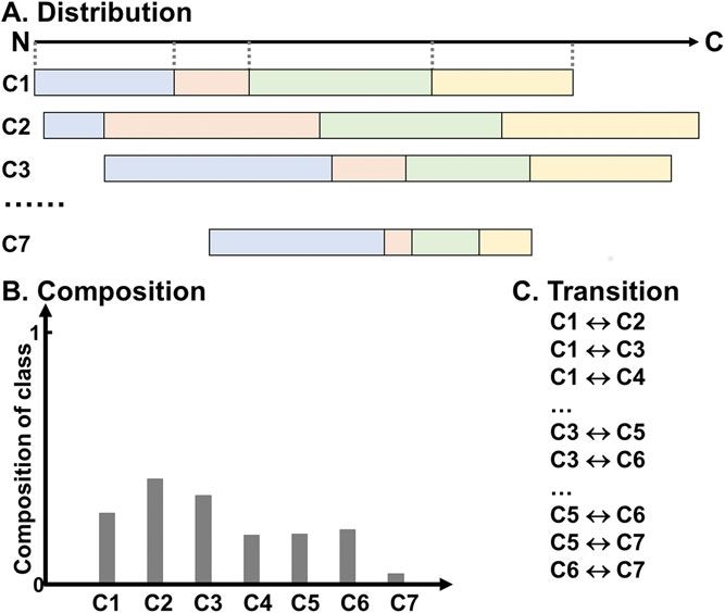
Besides using n-grams and its variants, there are several other ideas for capturing sequence
patterns that were used for PPI prediction. To capture general characteristics of a protein
sequence, a combination of three sequence features called the local descriptor was used
(Fig. 2; You, Chan, & Hu, 2015; Yang, Xia, & Gui, 2010; Zhou, Gao, & Zheng, 2011;
You, Lei, Zhu, Xia, & Wang, 2013). The features are the composition of amino acids,
transition probabilities between two consecutive amino acids, and a feature called the
distribution. The distribution describes the lengths of sequences from the N-terminus that
contain the first 25%, 50%, 75%, and 100% of each amino acid (class) over the sequence
(Dubchak, Muchnik, Holbrook, & Kim, 1995).
Guo et al. used a feature called auto covariance (AC) to represent protein sequences
(Guo, Yu, Wen, & Li, 2008). AC is intended to capture the periodicity of physicochemical
properties along a protein sequence (Fig. 3). To compute AC of a protein sequence
for a physicochemical property, amino acids are assigned with a property values, e.g.,
hydrophobicity, hydrophilicity, side-chain volume, polarity, solvent-accessible surface
area, or the net charge index of side chain. Then, AC is defined as follows:
L−lag L L
i=1 Pi, j − 1
L i=1 Pi, j × P(i+lag), j − 1
L i=1 Pi j
AC (lag, j) = ,
L − lag
Equation 2
where lag is the distance between covariant residues to consider, which ranges from 1
to 30, j is the j-th physiochemical descriptor, i is the position in the sequence, and L is
Ding and Kihara
the length of sequence. Thus, AC of a property with a certain lag length will be large if
6 of 27
Current Protocols in Protein ScienceFigure 2 The local descriptors. Amino acids are clustered into seven classes (C1-C7). (A) The
distribution of the lengths of sequences from the N-terminus that contain the first 25%, 50%,
75%, and 100% of each amino acid class in the protein sequence are represented in blue, pink,
green, and yellow, respectively. The dotted line represents the position of the first, first 25%, 50%,
75%, and 100% of Class 1 in the local region. The number of distribution descriptor is 7 (classes)
*5 (distribution values) = 35 for a local region. (B) The composition of each amino acid class in a
local region is considered. (C) The transition accounts for the frequency of the transition from one
class to another. The number of transition descriptor is (7*6)/2 = 21. Therefore, each local region
is represented by 35 + 7 + 21 = 63 descriptors.
Figure 3 Schematic view of calculating Auto-covariance (AC). The black line in the plot repre-
sents the value of the j-th physiochemical property along the amino acid sequence. The dashed
grey line represents the average value of the j-th physiochemical property. The grey bracket re-
gions are the difference from the average value of i-th and (i + lag)-th amino acid, respectively.
AC is the average of Fi , lag, j .
amino acids with a large (or small) property value appear periodically with an interval of
lag. There is a similar value called Moran auto correlation (MAC), which is defined as
N −d
1 1
N
2
M AC (d) = (P j − P̄) × (P j+d − P̄)/ P j − P̄ ,
N −d N
j=1 j=1
Equation 3
Ding and Kihara
7 of 27
Current Protocols in Protein Sciencewhere d is the distance between covariant residues, which ranges from 1 to 30, P j and
P j+d are the physiochemical property of j-th and (j+d)-th amino acid, respectively, N
N
Pj
is the length of the protein sequence, P̄ = j=1 N is the average value of the phys-
iochemical property (You et al., 2013). Thus, MAC is AC divided by variance of the
physiochemical property, N1 Nj=1 (P j − P̄)2 .
The intention behind computing the local descriptor, AC, and MAC is to capture global,
long range sequence features of proteins, in contrast to n-gram and its variants, which
captures local patterns of sequences. As these features are complementary to each other,
often both types were combined (Ding et al., 2016). For example, in the method by
You et al., there were four components in the protein sequence feature representation
(You et al., 2013). First, 3-grams, where amino acids were classified to seven classes
and the frequency of 3-grams was considered as a feature of a protein; thus, a protein
pair is represented by a vector of 686 (= 2*7*7*7) features. Second, AC, with six
physicochemical properties of amino acids being considered (hydrophobicity, side-chain
volume, polarity, polarizability, solvent-accessible surface area, and the net charge of
the side chains). For each of the properties, AC was computed using 1 to 30 lag values
following Eq. 2; thus, the length of the vector for a protein pair was 360 (= 2*6*30).
Third, MAC, where, similar to AC, a 360-dimension vector was constructed for a protein
pair. Fourth, local descriptors, where amino acids were classified to seven classes and
the local descriptor, the composition, the transition, and the distribution, were computed
for each of the seven amino acid classes for ten local regions in a protein. Thus, a pair of
proteins were represented by a vector of 1260 = 2* 10* (7 compositions + 21 transitions
+ 35 distributions) values. Overall, considering all four features, a protein pair was
represented by a vector of 2666 (= 686 + 360 + 360 + 1260) features.
With these sequence features, predictions of PPIs were made using various machine
learning algorithms. Algorithms used include support vector machine (SVM; Bock &
Gough, 2001; Y. Guo et al., 2008; X. Liu et al., 2012; Martin et al., 2005; Shen et al.,
2007; Y. Z. Zhou et al., 2011), relevance vector machine (An et al., 2016), random
forest (X.-W. Chen & Liu, 2005; Ding et al., 2016; You et al., 2015), rotation forest
(L. Wong et al., 2015), linear discriminant classifier and cloud points (Nanni, 2005),
relaxed variable kernel density estimator (RVKDE; C.-Y. Yu et al., 2010), an ensemble
classifier (L. Wei et al., 2017), extreme learning machine (ELM; You et al., 2013), and
k-nearest neighbors (KNNs; Yang et al., 2010).
These sequence-based methods reported surprisingly high accuracies. For example, Shen
et al., reported 83.90% accuracy on the HPRD dataset (Prasad et al., 2009; Shen et al.,
2007). Yang et al. reported 86.15% accuracy on a yeast dataset (Yang et al., 2010). Yu
et al. achieved 93.7% accuracy on a highly unbalanced HPRD dataset where positive-to-
negative ratio was 1:15 (C.-Y. Yu et al., 2010). Zhu et al. reported over a 75% accuracy on
five organisms including yeast, C. elegans, E. coli, human, and mouse (Y. Z. Zhou et al.,
2011). Wong et al. achieved 93.92% on the S. cerevisiae dataset (L. Wong et al., 2015).
You et al. achieved 93.46% to 97.01% accuracy on six different organisms including
yeast, Helicobacter pylori, C. elegans, E. coli, human, and mouse (You et al., 2015).
Ding et al. achieved 95.01% on the yeast dataset and 87.59% on the H. pylori dataset
(Ding et al., 2016). An et al. achieved 94.57% and 90.57% on the S. cerevisiae and the
H. pylori dataset, respectively; also, a 97.15% accuracy on an imbalanced yeast dataset
(An et al., 2016). Wei showed over 81% accuracy using different features on the Negatome
and the DIP dataset (Blohm et al., 2014; L. Wei et al., 2017; Xenarios et al., 2002).
Although the reported accuracy values are high and encouraging, it needs to be noted
that the datasets on which the methods are tested are limited to several organisms.
Ding and Kihara
8 of 27
Current Protocols in Protein ScienceUsing homology
So far, we have reviewed methods that use partial sequence patterns and statistical fea-
tures in protein sequences. In this section, we introduce methods that use the similarity
of entire protein sequences. Many functionally important proteins in an organism are
conserved across species, which is the rationale of sequence similarity search for anno-
tating function of genes (Chitale, Hawkins, Park, & Kihara, 2009; T. Hawkins, Chitale,
Luban, & Kihara, 2009; Troy Hawkins & Kihara, 2007). Several databases, such as Kyoto
Encyclopedia of Genes and Genomes (KEGG) Orthology (Tanabe & Kanehisa, 2012),
OrthoDB (Waterhouse, Tegenfeldt, Li, Zdobnov, & Kriventseva, 2013), OrthoMCL-DB
(F. Chen, Mackey, Stoeckert, & Roos, 2006), HomoloGene (NCBI, 2016), and INPARA-
NOID (Sonnhammer & Ostlund, 2015), contain lists of precomputed homologous genes
in different species. As interactions with other proteins is a part of a protein’s function,
it is known that PPIs are often conserved across species. These conserved interactions
are noted as “interlogs” (Walhout et al., 2000). Matthew et al. mapped PPIs in the yeast
interaction map to predict PPIs in C. elegans, and identified 257 potential interlogs
(Matthews et al., 2001). Further experimental validation performed on 72 predicted in-
teractions gave 19 positive results, which were roughly 25% among tested. The POINT
web service provides human PPIs inferred from interlogs with mouse, fruitfly, yeast,
and C. elegans (T.-W. Huang et al., 2004). Taking advantage of an increasing number of
experimentally identified protein interactions, Lee et al. then expanded orthologous pairs
to consider those from 18 eukaryotic species (Lee et al., 2008). The idea of interlogs was
also applied to predict PPIs in the plant, A. thaliana, by considering homologs with yeast,
fruitfly, human, and C. elegans (Geisler-Lee et al., 2007; De Bodt, Proost, Vandepoele,
Rouzé, & Van de Peer, 2009) and to a second plant, Oryza sativa (Asian rice), by consid-
ering interlogs with the six species including the same four species with E. coli and A.
thaliana (Gu, Zhu, Jiao, Meng, & Chen, 2011). Dutkowski et al. developed a statistical
model, which represents specification and duplication events of genes along an evolution-
ary tree, on which known interacting protein pairs in seven eukaryotic organisms were
mapped and used for predicting PPIs (Dutkowski & Tiuryn, 2009). Interactome3D is a
database that provides the tertiary structure models of protein complexes built based on
known structure information of interlogs (Mosca, Pons, Céol, Valencia, & Aloy, 2013).
Wang et al. merged prediction results from an interlog-based method and a motif-based
method to cover a larger number of predicted PPIs in the pig proteome (Wang et al.,
2012).
Codon usage
Interestingly, it was shown that the codon usage of genes can be used to predict PPIs.
Using the difference of codon usage of protein pairs, Najafabadi et al. predicted PPIs in
E. coli, yeast, and Plasmodium falciparum with reasonably good accuracy (Najafabadi
& Salavati, 2008). For a pair of genes i and j the difference in usage of codon c among
64 codons is simply defined as
di j (c) = f i (c) − f j (c)
Equation 4
where fi (c) is the usage of codon c of gene i. Then, dij of each codon is binned into
50 intervals, and the likelihood ratio of the fraction in interacting and non-interacting
proteins in a training dataset was computed. A PPI prediction for a protein pair is
performed with a naı̈ve Bayes approach using the likelihood ratio. Zhou et al. used
SVM with the codon usage difference and applied to the yeast genome (Zhou, Zhou, He,
Ding and Kihara
Song, & Zhang, 2012). One may wonder why codon usage is related to PPIs. But it is
9 of 27
Current Protocols in Protein ScienceFigure 4 Comparative genomics-based methods. (A) Phylogenetic tree topology-based method.
A pair of query sequences, A and B, are compared with n reference organisms and multiple
sequence alignments are constructed. Based on the alignments, phylogenetic trees are computed,
from which distances between all pairs of sequences are computed and stored in matrices. Then
the similarity between two matrices is evaluated with a correlation coefficient. (B) Phylogenetic
profiles. Genes in a query organism is compared with n reference organisms by BLAST search. 1
represents the presence of the gene in the reference organism 0 for the absence. The table can
also be filled with real-values, such as BLAST bit scores. (C) Gene fusion. Two protein genes A
and B are predicted as interacting if they fuse to form one protein gene AB in another organism.
(D) Gene order. If protein gene orders of proteins are conserved among different species, they
are predicted as interacting proteins with each other.
reasonable considering that codon usage is known to be correlated with gene expression
levels (Jansen, Bussemaker, & Gerstein, 2003) and also that neighboring genes have
similar codon usage. As we discuss later in this review, both gene expression level and
conserved neighboring genes (gene order) have been successfully used to predict PPIs.
COMPARATIVE GENOMICS-BASED METHODS
The last level of sequence information that can be used for PPI prediction is from genome
sequences from various species. Since important features in a genome sequence are
conserved during evolution, identifying such conserved features in genomes can be a clue
for identifying proteins that are functionally related. Under this category, which we call
the comparative genomics-based methods, we discuss four approaches, the phylogenetic
tree topology analysis, the phylogenetic profile, considering gene fusion events, and
conserved gene orders (Fig. 4). An important point to note is that these methods are not
Ding and Kihara
aimed toward predicting physical PPIs directly but for identifying functionally related
10 of 27
Current Protocols in Protein Scienceproteins. Quite often, however, functionally related proteins do physically interact with
each other. A strong advantage of the comparative genomics-based approaches is that,
due to the increasing number of determined genome sequences, many proteins can now
find related (and maybe interacting) proteins through these approaches (Huynen, Snel,
von Mering, & Bork, 2003).
Phylogenetic Tree Topology Analysis
It has been observed that the phylogenetic trees between interacting proteins are more
similar than a general divergence between the corresponding species (Goh & Cohen,
2002; Goh, Bogan, Joachimiak, Walther, & Cohen, 2000; Pazos & Valencia, 2001).
The similarity between the phylogenetic trees of interacting proteins was explained as
maintenance of the complex functionality and suffering similar evolutionary pressure.
The sequence signal of coevolution is strong at the binding interface of proteins but can
also be detected other regions of proteins (Kann, Shoemaker, Panchenko, & Przytycka,
2009).
The tree topology similarity can be measured as the correlation between the evolutionary
distance matrices used to build the trees. The algorithm to calculate similarity of distance
matrices is called the mirror tree method (Pazos & Valencia, 2001). It contains the
following steps (Fig. 4A): 1) Construct a multiple sequence alignment for each protein
against a list of reference organisms; 2) Construct a phylogenetic tree for the proteins; 3)
Then, for a pair of proteins in question, distances against orthologous proteins in different
species are computed (distance matrices) and the correlation coefficient between two
distance matrices is obtained. A protein pair is predicted to be interacting if the coefficient
value is above a cut-off value, which is determined to distinguish known interacting and
non-interacting proteins.
The mirror tree method was modified for improvement in several different ways. The
method was extended to handle interacting protein families, such as a ligand family
and a receptor family, to be able identify interacting specific protein pairs from the two
families (Ramani & Marcotte, 2003). Sato et al. removed a background tree similar-
ity that arises by the overall evolutionary distance of organisms from distance matrices
of individual proteins, which yielded improvement of PPI prediction accuracy (Sato,
Yamanishi, Kanehisa, & Toh, 2005). They further considered partial correlation of dis-
tance matrices that can more effectively remove background organism-level similarity
from the tree similarity of a query protein pair, where the background organism-level
similarity was represented by a linear combination of distance matrices of many pro-
teins in the organisms (Sato, Yamanishi, Horimoto, Kanehisa, & Toh, 2006). Besides the
background similarity of organisms, another source of noise in the mirror tree method
is that a protein coevolves with multiple interacting proteins. Instead of evaluating tree
similarity of a query protein pair, Juan et al. considered a network of similarities between
all pairs of proteins simultaneously (Juan, Pazos, & Valencia, 2008). In the mirror tree
method, selection of reference genomes is a key for successful prediction. Effective ways
to select organisms for building trees were examined by Herman et al. (Herman et al.,
2011). Instead of using correlation coefficient, SVM was also used to make predictions
from distance matrices (Craig & Liao, 2007).
Phylogenetic Profiles
Phylogenetically related and thus possibly interacting protein pairs can be identified in a
simpler way using comparative genomics. In the approach called the phylogenetic profil-
ing, co-presence and co-absence of orthologous proteins across organisms are examined
rather than comparing phylogenetic trees of protein pairs as discussed in the previous
Ding and Kihara
section (Pellegrini, Marcotte, Thompson, Eisenberg, & Yeates, 1999). If two proteins are
11 of 27
Current Protocols in Protein Scienceneeded for realizing a certain biological function, an organism needs to possess both pro-
teins if the function is required, while both proteins are not needed if the organism does
not require the function. Coding one of the proteins only in its genome is meaningless.
There are three major steps to perform this method (Fig. 4B). The first step is to identify
orthologous proteins for all the proteins in a query genome against other reference
genomes by a sequence similarity search. Then, a phylogenetic profile is constructed for
each protein in the query genome, which has binary values with 1 indicating the presence
of an orthologous gene and 0 for the absence of the ortholog in a reference genome.
Thus, the dimension of the profile is the number of reference genomes used. Finally,
protein pairs that have similar profiles are predicted to be interacting (more precisely,
functionally related). Similar to the phylogenetic tree topology methods, the choice of
reference genome is crucial for this approach (Sun, Li, & Zhao, 2007). Also, a threshold
value (E-value) in sequence similarity search for detecting orthologous proteins strongly
affects the profiles, and thus the prediction performance of the method (Sun et al., 2005).
To accommodate the strong dependency of the performance to the threshold value in
the similarity search, real value vectors of an alignment score was used for constructing
profiles rather than binary values (Lin, Wu, & Chang, 2013). In the method by de Vienne
and Azé, a combination of the phylogenetic tree topology and profile was used as features
in a machine learning framework (de Vienne & Azé, 2012).
Gene Fusion Events
A gene fusion refers to an event in the comparative genomics where two individual
genes in one organism fuse as a continuous sequence in another organism (Snel, Bork, &
Huynen, 2000) (Fig. 4C). Fused genes are usually functionally related and further implies
physical interactions between the proteins (Enright, Iliopoulos, Kyrpides, & Ouzounis,
1999; Marcotte et al., 1999; Yanai, Derti, & DeLisi, 2001). Computationally, fused genes
can be found by gene sequence similarity search between genomes. It was reported that
metabolic enzymes are frequently involved in gene fusions (Tsoka & Ouzounis, 2000).
Conserved Gene Orders
Through evolution, genomes undergo various rearrangements and transfers; therefore,
locations of genes in a genome tend to be shuffled unless an evolutionary pressure keeps
the order of some genes together (Suyama & Bork, 2001; Fig. 4D). Thus, conservation
of gene orders, i.e., common local clusters of genes in genomes, indicates that there is a
requirement or an advantage to keep the gene order for the organisms, and in fact in many
cases, genes in a conserved cluster are involved in the same function (Tamames, Casari,
Ouzounis, & Valencia, 1997). In bacterial and archaeal genomes, operon structures are
conserved across many species, which code genes in the same pathways or complexes
(Dandekar, Snel, Huynen, & Bork, 1998). After initial findings of the conserved gene
orders, more systematic studies have been done (Fujibuchi, Ogata, Matsuda, & Kanehisa,
2000; Overbeek, Fonstein, D’souza, Pusch, & Maltsev, 1999). Similar to the other com-
parative genomics-based methods, a key for successful application of this analysis is to
choose an appropriate set of reference genomes, which should not be too evolutionarily
distant but not too close to each other, so that only clusters of functionally related genes
are conserved. A related work was done by Kihara & Kanehisa where transmembrane
protein complexes were predicted from genomes by identifying gene clusters that have
predicted transmembrane domains (Kihara & Kanehisa, 2000).
FUNCTION-BASED METHODS
Since interacting proteins belong to the same pathway and share function, functional
similarity of proteins can be a clue for predicting PPIs. Functional similarity of proteins
Ding and Kihara
is usually quantified by a similarity score of Gene Ontology (GO) terms (Consortium,
12 of 27
Current Protocols in Protein Science2017) that annotate the proteins. Similarity of GO terms are defined by the closeness
of the terms on the GO hierarchy tree and/or the frequency of the GO terms in gene
annotations observed in an protein annotation database, e.g., UniProt (Lin, 1998; Resnik,
1995; Schlicker, Domingues, Rahnenführer, & Lengauer, 2006) (Wu, Pang, Lin, & Pei,
2013). Interestingly, it was shown that considering common children terms of GO terms
in addition to common parental GO terms, which are not used in the aforementioned
functional similarity scores, improved PPI prediction accuracy (Zhang & Tang, 2016).
Jain and Bader defined a GO similarity score by considering the distance to the leaf nodes
in order to reduce the influence of imbalanced branch depths in the GO hierarchy (Jain
& Bader, 2010).
GO term similarity (or relevance) can be also defined by counting frequency of co-
occurrence of GO term pairs in biological contexts, in gene annotation, or PubMed
abstracts (Chitale, Palakodety, & Kihara, 2011), or in known PPIs (Wei, Khan, Ding,
Yerneni, & Kihara, 2017; Yerneni, Khan, Wei, & Kihara, 2015).
Since PPI prediction is a suitable and handy application of GO term similarity scores,
all the GO term scores above have been tested and compared for their performance of
PPI predictions (Guo, Liu, Shriver, Hu, & Liebman, 2006; Jain & Bader, 2010; Wu
et al., 2013; Yerneni et al., 2015). Maetsche et al. showed that when using GO terms
for PPI prediction in machine learning framework, induced GO term sets, e.g., common
parental terms of annotated GO terms, performed better rather than using the original
GO annotations of proteins (Maetschke, Simonsen, Davis, & Ragan, 2012).
GENE CO-EXPRESSION-BASED METHODS
Gene co-expression data such as microarray and RNA-sequencing data are valuable
experimental data that can be used to infer PPIs. Intuitively, interacting protein pairs
are expected to have similar gene expression levels across different conditions. Indeed
significant correlation between the gene co-expression level and PPIs was shown in
bacteriophage T7 (Grigoriev, 2001), yeast (Ge, Liu, Church, & Vidal, 2001; Jansen,
Greenbaum, & Gerstein, 2002), human, mouse, and E. coli (Bhardwaj & Lu, 2005).
Fraser et al. showed that gene expression level of interacting proteins co-evolve using
four closely related yeast species, where the expression level was estimated by the
codon usage (Fraser, Hirsh, Wall, & Eisen, 2004). Databases that provide large-scale
gene co-expression information include GEO (Barrett et al., 2013), ATTED-II (Aoki,
Okamura, Tadaka, Kinoshita, & Obayashi, 2016), and COXPRESdb (Okamura et al.,
2014). ATTED-II and COXPRESdb are pre-calculated gene co-expression databases of
plant organisms and animal species, respectively.
Although gene expression is shown to have significant correlation to PPIs, a major
challenge is that co-expression data is noisy due to various types of systematic and
stochastic fluctuations. Soong et al. adopted principle component analysis (PCA) and
independent component analysis (ICA) to filter out noise in microarray data before
feeding the data to SVM classifier (Soong, Wrzeszczynski, & Rost, 2008). As we see
later in the section for integrated methods, gene expression is used frequently as one of
the input features for proteins.
PROTEIN TERTIARY STRUCTURE-BASED METHODS
The tertiary (3D) structure of proteins can be important information to predict PPIs,
if available, or if the structures can be computationally reliably modelled. There
are many computational methods developed that “docks” two protein structures to
provide the tertiary structures of a protein complex from individual protein struc-
Ding and Kihara
tures, which include LZerD (Esquivel-Rodriguez, Filos-Gonzalez, Li, & Kihara, 2014;
13 of 27
Current Protocols in Protein ScienceEsquivel-Rodrı́guez, Yang, & Kihara, 2012; Peterson, Roy, Christoffer, Terashi, & Ki-
hara, 2017; Venkatraman, Yang, Sael, & Kihara, 2009), GRAMM-X (Tovchigrechko
& Vakser, 2006), ZDOCK (Pierce et al., 2014), RosettaDock (Lyskov & Gray, 2008),
HADDOCK (Geng, Narasimhan, Rodrigues, & Bonvin, 2017), SwarmDock (Torchala
& Bates, 2014), HEX (Ritchie & Kemp, 2000), and ClusPro (Kozakov et al., 2017).
These docking methods build structure models of a protein complex given individual
protein structures, which provide structural insights of the PPI. However, it should be
noted that these docking methods do not predict whether a protein pair actually interacts
or not.
How then does one use structure information for predicting PPIs? There are two ap-
proaches explored. The first approach is to detect energetic characteristics of interacting
protein pairs observed in protein docking prediction. A protein docking program typically
generates over tens of thousands of different docking poses for a pair of input protein
structures. Wass et al. reported the score distribution of docking poses of interacting
protein pairs can be distinguished from those of non-interacting proteins, because the
former distribution is skewed toward favorable scores (Wass, Fuentes, Pons, Pazos, &
Valencia, 2011). This is an intriguing observation because a docking pose distribution
include both near-native (i.e., almost correct) and incorrect poses, therefore, the report
implies that even incorrect docking poses have relatively favorable scores (i.e., more
favorable geometric complementary) in cases of interacting proteins. In MEGADOCK,
a protein docking method aimed for fast, large-scale protein docking screening, a protein
pair is predicted to be interacting if a pool of docking poses generated by the algo-
rithm include clusters of similar poses that have significantly favorable docking scores in
comparison with the rest of the poses (Ohue, Matsuzaki, Uchikoga, Ishida, & Akiyama,
2014).
The second approach to use protein structure information for PPI prediction is, for two
query protein structures, to find similarity in known protein complexes. PRISM, devel-
oped by Keskin and his colleagues, is one of the first to take this approach (Aytuna,
Gursoy, & Keskin, 2005; Tuncbag, Gursoy, Nussinov, & Keskin, 2011). PRISM takes
two protein structures as input, and examines if surface shapes of the proteins have sim-
ilarity to docking interfaces from known protein complexes structures. To perform this
comparison, PRISM has a database of docking interface regions of known protein com-
plexes extracted from the PDB database (Rose et al., 2017). Identified potential interface
regions in the two query proteins that are identified by comparison to known interface
regions are examined for structural similarity to the template, sequence conservation, and
the binding energy. Although the prediction power of PRISM relies on the coverage of
template dataset, the method will be able identify interactions between proteins that are
globally dissimilar but have similar local interface regions to known protein complexes.
PrePPI takes a similar approach to PRISM (Q. C. Zhang et al., 2012). One difference is
that PrePPI takes sequences of the query proteins and models their structures by homol-
ogy modeling. Subsequently, the two structures are mapped to known protein complex
structures, which are then evaluated by structure and sequence similarity scores to the
known complex structures. Final prediction is made by a composite score that integrates
five other features, gene co-expression, essentiality of the proteins, functional similarity,
and the phylogenetic profile. Similarly, Coev2Net models a complex structure of two
query proteins by mapping their sequences to a known complex structure with a thread-
ing method, and then evaluates the complex model by a logistic regression classifier that
considers structural and sequence features taken from its interface (Hosur et al., 2012). In
a recent method, InterPred, a similar approach is taken (Mirabello & Wallner, 2017): for
a query protein sequence pair, structures are modelled, then known protein complexes
are sought by structure comparison. Finally, the feasibility of the model is evaluated
Ding and Kihara using a random forest classifier that considers interface structure and sequence features
14 of 27
Current Protocols in Protein ScienceTable 2 Lists of Available Information Such as Number of Coding Genes, Number of Genes with
Annotated GO Terms, Genes with Co-expression Information, Number of Solved Structure, and Number
of Redundant Modeled Structure, in Each Organism
Fraction of
# of genes modeled
# of genes # of proteins with # of proteins structure
with protein with annotated co-expression with a solved among all
Organism productsa GO termsb informationc structured proteins (%)e
Human 109,018 46,331 19,816 16620 82.21
Yeast 6,002 5,582 4,461 1340 90.25
Mouse 76,216 28,727 20,403 2891 84.07
A. thaliana 48,350 16,123 20,836 584 77.44
Fruitfly 30,482 6,886 13,099 875 88.92
Asian rice 28,555 100 20,625 1 NAf
X. tropicalis 39,662 1,998 11,095 10 91.06
D. rerio 46,451 2,723 10,112 26 NA
C. annuum 45,410 20 17,453 0 NA
P. persica 28,927 2 11 0 NA
a Counted in the NCBI reference sequence (RefSeq) (Pruitt, Tatusova, & Maglott, 2005).
b Protein entries in RefSeq was mapped to UniProt, where the number of proteins with at least one annotated Gene Ontology term
was counted (Boutet et al., 2016).
c Gene expression data of human, yeast, mouse, fruitfly, and D. rerio were taken from COXPRESdb (Okamura et al., 2014). Data
for A. thaliana and O. Sativa were taken from the ATTED-II database (Aoki et al., 2016). Expression data for the rest of the three
organisms were taken from literature: X. tropicalis: (Yanai, Peshkin, Jorgensen, & Kirschner, 2011). C. annuum: (Sharma, 2016).
P. persica: (Tong, Gao, Wang, Zhou, & Zhang, 2009).
d After mapping RefSeq IDs of protein genes to UniProt, the number of proteins was counted with at least one crosslinked PDB
entry (Boutet et al., 2016).
e It is computed from the statistics provided in the ModBase base (Pieper et al., 2006).
f NA indicates that no modeled structures provided on ModBase (but some proteins in a genome may be modelled by a standard
modeling procedure).
as well as overall structure similarity between individual models to the template complex
structure.
Although protein structures can provide unique features for PPI prediction, a drawback
is that not many proteins have known structures. In Table 2, the number of protein genes
with GO terms, gene expression data, and experimentally determined/computationally-
modelled protein structures for ten genomes are shown. Compared to GO terms and gene
expressions, proteins with known structures are substantially fewer. This is more evident
for genomes that are less studied. On the other hand, as shown in the right-most column,
most of the protein structures can be computationally modelled (Kihara & Skolnick,
2004). Thus, there is room for new structure-based approaches that use modelled protein
structures.
PPI NETWORK TOPOLOGY-BASED METHODS
Methods in this category start from an existing PPI network of an organism and predict
new interactions between proteins by evaluating their network topology features. In the
IRAP* method, a missing interaction is predicted if a protein pair has a high score
that reflects the number of common neighbors between them in the current PPI network
(Chen, Hsu, Lee, & Ng, 2006). Another idea by Yu et al. is to predict a PPI if two proteins
are neighbors of a clique, a fully-connected graph, in the PPI network of the organism and
Ding and Kihara
connecting them would complete a larger clique, because most probably the two proteins
15 of 27
Current Protocols in Protein Scienceare subunits of a protein complex (Yu, Paccanaro, Trifonov, & Gerstein, 2006). In the
work by L. Wong and his colleagues, a prediction of a PPI is made using a combination
of two scores, a score for capturing local network topology of proteins that is based on
the number of common neighbors and a global topology-based score that accounts for
the memberships of the proteins in protein groups where member proteins interact with
each other (Liu, Li, & Wong, 2008). Kuchaiev et al. applied Multi-Dimensional Scaling
(MDS), a dimension reduction method in statistics, to a PPI network, where distances are
based on edge distances between proteins (Kuchaiev, Rašajski, Higham, & Pržulj, 2009).
New PPIs are predicted if proteins are closer than a threshold in the projected space
by MDS. Lei and Ruan applied a random walk-based approach, where the probability
of reaching each node from each of the other nodes in the network is computed by
assuming a random walk (Lei & Ruan, 2012). The resulting probability matrix contains
information of the topology of the PPI network. Based on the probability matrix, protein
pairs are connected if they are similar in their probability vectors to reach the other
nodes.
INTEGRATION OF MULTIPLE FEATURES
PPIs can be predicted from different perspectives as discussed above. Naturally, there are
methods that use multiple features to be able to combine strengths of different features
and to increase the prediction confidence and coverage. Features can be combined using
machine learning methods, such as random forest, Naı̈ve Bayesian Network, artificial
neural network, SVM, and logistic regression (Qi, Bar-Joseph, & Klein-Seetharaman,
2006). In Table 3 methods that use multiple features are summarized.
From the table, we can see the most popular feature integrated was gene co-expression
data (COX). The next most popular ones are GO functional similarity (GO), and ho-
mology (HOM). Several features in the table are not explained yet in this review. The
physicochemical features (PCH) concerns features such as charge and aromaticity of
amino acids in a protein sequence. The post-translational modification feature (PTM)
indicates that PTM motifs are found in UniProt and HPRD. The disordered region (DIS)
is a protein structure feature where non-structured regions in a protein can be predicted
from its sequence. Thus, besides obvious sequence-based features, DIS, PCH, and PTM
are features that are predicted from protein sequences. Direct experimental data of PPIs
(EXP) used by Qi et al. were yeast-two-hybrid and mass spectrometry data (Qi et al.,
2006), and those used by Miller et al. were data from yeast two-hybrid system (Miller
et al., 2005). The protein functional class (CLA) in yeast are taken from the Munich
Information Center for Protein Sequences (MIPS) Protein Class Catalogue, which were
determined by experiments (Mewes et al., 2004). Gene essentiality (ESN), synthetic
lethality (SNL), and MIPS mutant phenotype (MUT) were determined by knockout
mutants (Qi et al., 2006). Text mining (TXT) counts co-mentions of two proteins in
PubMed abstracts.
Regarding combinations of features, methods by Ben-Hur et al., Xu et al. combine mostly
sequence-based features (Ben-Hur & Noble, 2005; Xu et al., 2010). On the other hand,
PrePPI (Q. C. Zhang et al., 2012), FpClass (Kotlyar et al., 2015), and Taghipour et al.
(Taghipour, Zarrineh, Ganjtabesh, & Nowzari-Dalini, 2017) are intended to combine
different types of features.
Turning our attention to algorithms used, naı̈ve Bayes is the most frequently used among
the multiple feature-based methods in Table 3. SVM was the next, used in the three
methods. Qi et al., tested five integrating algorithms with different feature combinations
(Qi et al., 2006).
Ding and Kihara
16 of 27
Current Protocols in Protein ScienceTable 3 Features and Algorithms Used in Multiple-Feature Integrative Methods
Ben- Taghi- # of
Hur Miller Scott Xu STRI- pour times
Feature et al.a et al.b Qi et al.c et al.d et al.e PAIRf PrePPg FpClash NGi et al.j used
Sequence MOT/DOM X X X X X X 6
NGM X 1
PCH X 1
Current Protocols in Protein Science
HOM X X X X X X X 7
COD X 1
PHP X X X X X 5
FUS X X X 3
GNB X X X 3
PTM X X 2
Function GO X X X X X X X X 8
MIPS X 1
Experiment COX X X X X X X X X X 9
XPI X X 2
CLA X 1
ESN X X X 3
LOC X X X 3
COR X 1
SNL X 1
MUT X 1
continued
17 of 27
Ding and Kihara18 of 27
Ding and Kihara
Table 3 Features and Algorithms Used in Multiple-Feature Integrative Methods, continued
Ben- Taghi- # of
Hur Miller Scott Xu STRI- pour times
Feature et al.a et al.b Qi et al.c et al.d et al.e PAIRf PrePPg FpClash NGi et al.j used
Structure STR X 1
DIS X 1
Network NET X X X X X 5
Literature TXT X 1
Integrating method LPK SVM RF, KNN, NB, NB NB SVM NB NOR LNR NB,
DT, LR, SVM MCL
References of each method
a Ben-Hur & Noble, 2005
b Miller et al., 2005
c Qi et al., 2006
d Scott & Barton, 2007
e Xu et al., 2010
f Lin, Shen, & Chen, 2011
g Q. C. Zhang et al., 2012
h Kotlyar et al., 2015
i D. Szklarczyk et al., 2017
j Taghipour et al., 2017
Feature abbreviations: MOT/DOM: protein motifs or domains; NGM: n-gram; PCH: physiochemical feature; HOM: homologous interaction (interlogs); COD: codon usage; PHP:
phylogenetic profile and gene co-occurrence; FUS: gene fusion; GNB: gene neighbor; PTM: post-translational modifications regions; GO: gene ontology terms; MIPS: Munich Information
Centre for Protein Sequences (MIPS) functional similarity; COX: gene/protein co-expression; XPI: Experimental PPI detection, direct experimental data including two-hybrid screens and
mass spectrometry; CLA: protein functional class by MIPS Protein Class Catalogue; ESN: essentiality; LOC: protein localization; COR: common co-regulators of genes; SNL: synthetic
lethality; MUT: MIPS mutant phenotype; STR: protein structure; DIS: disordered region; NET: protein-protein interaction network; TXT: text mining. Integrating method abbreviations:
LPK: linear pairwise kernel; SVM: support vector machine; RF: random forest; KNN: k-nearest neighbor; NB: Naı̈ve Bayes; DT: decision tree; LR: logistic regression; NOR: noisy-OR
model (a type of Bayesian network); LNR: linear regression; MCL: Markov clustering algorithm.
Current Protocols in Protein ScienceYou can also read