COUNTERFACTUAL RISK ANALYSIS OF TROPICAL CYCLONES
←
→
Page content transcription
If your browser does not render page correctly, please read the page content below
COUNTERFACTUAL RISK ANALYSIS OF
      TROPICAL CYCLONES

                  MASTER THESIS
  OESCHGER CENTRE FOR CLIMATE CHANGE RESEARCH
      FACULTY OF SCIENCE, UNIVERSITY OF BERN

                 handed in by
         TAMARA ALESSANDRA BAUMANN

                     2022

                    Supervisor:
      PROF. DR. OLIVIA ROMPPAINEN-MARTIUS

                    Advisor:
               DR. ALESSIO CIULLO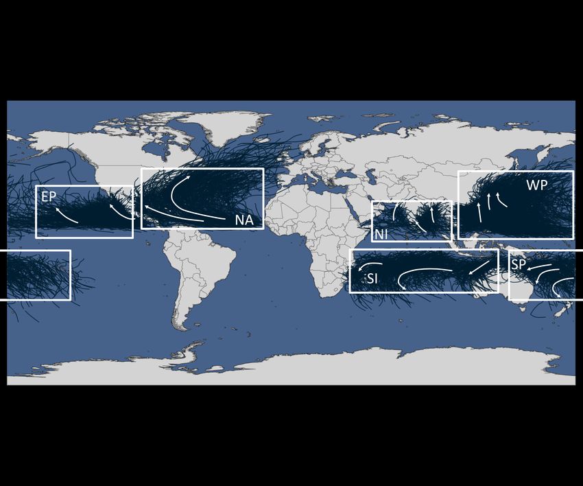
Abstract
Tropical cyclones (TC) are among the most devastating natural hazards causing losses and
damages in almost all tropical regions. However, an accurate risk analysis of TC in these
regions is not straightforward due to sparse data availability and short observational records.
High impact extreme events at the tail of the distribution are often underestimated and biased
towards the outcome of past events. The goal of counterfactual risk analysis is to improve risk
assessment of extreme events by incorporating data on near-miss events. Considering the
chaotic nature of atmospheric dynamics, the outcome of past TC can be viewed as only one of
many possible realizations. By incorporating alternative but physically plausible scenarios of
past events, so called counterfactuals, the sparse observational datasets of TC can be improved
significantly.
Within this thesis, TC forecasts of past events are used as a source to create counterfactual
scenarios of past yearly landfall rates. By identifying possible landfalls of observed events and
worst-case scenarios, downward counterfactuals are established and compared to observed
landfall rates using Bayesian inference.
The analysis of downward counterfactual scenarios leads to a higher estimation of expected
mean yearly landfall rates, probability of extreme events and outliers, and future annual landfall
rates, including its extremes. TC forecasts allow the detection of near-miss events and
expansion of the sparse observational data, especially for small island states where TC landfalls
are rare. The results highlight that counterfactual data is promising in improving the risk
assessment of TC at the tail of the distribution. The results also show that TC forecasts can be
a great source in building counterfactual scenarios.

                                                                                                2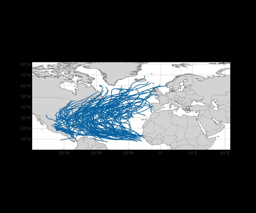
Abbreviations
BI ................................................................................................................... Bayesian inference
CF .......................................................................................................................... counterfactual
ECMWF ..............................................European Centre for Medium-Range Weather Forecasts
EP .............................................................................................................................. East Pacific
IBTrACS ......................................... International Best Track Archive for Climate Stewardship
KWBC ................... National Centres for Environmental Prediction (USA) and Meteorological
   Service of Canada
LF ..................................................................................................................................... landfall
NA ......................................................................................................................... North Atlantic
NI .................................................................................................................. North Indian Ocean
NOAA ........................................................ National Oceanic and Atmospheric Administration
PP .............................................................................................. posterior predictive distribution
SI .................................................................................................................. South Indian Ocean
SP ............................................................................................................................South Pacific
TC ...................................................................................................................... Tropical cyclone
THORPEX .............................. The Observing System Research and Predictability Experiment
TIGGE .............................................................. THORPEX Interactive Grand Global Ensemble
WP ............................................................................................................................ West Pacific

Variables
! .................................................................................................... observed yearly landfall rate
" ........................................................................................................... number of years observed
λ ..................................................................................................................... mean landfall rate
$(&) .................................................................................................................... prior probability
$(&|!) ......................................................................................................... posterior probability
$( &|!!"# ) .................................................................posterior belief for λ given observed y 2008-2019
$( &|!$%&'( ) .......................... posterior belief for λ given worst-case counterfactual y 2008-2019
$(!|&) ............................................................................................................... likelihood, model
$(!) ............................................................................................................ marginal distribution
$(!+|y) ........................................................................................ posterior predictive distribution
- [&] .............................................................................................................. expected value for λ
0, 2 ........................................................... shape and rate, hyperparameters gamma distribution
                                                                                                                  3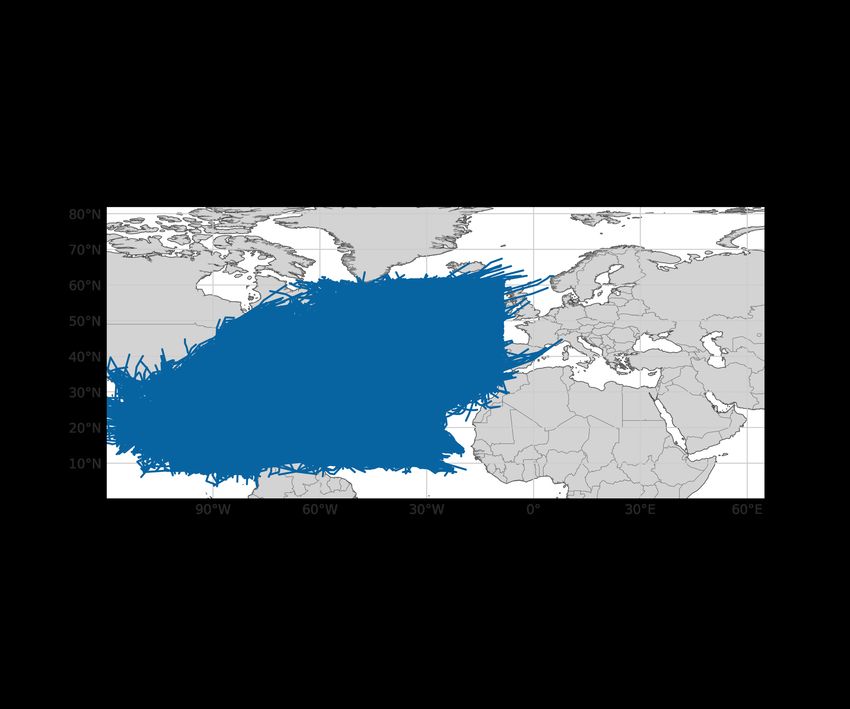
!345 ................................................................ highest observed yearly landfall rate up to 2007
6)*#+ ................................................................................ mean observed landfall rate up to 2007
6)*#+,- ........................................................................... mean observed landfall rate 1950-2007
6)*#+.-         ...................................................................... mean observed landfall rate 1980-2007
$(&,- ) ................................................ prior probability based on observation period 1950-2007
$(&.- ) ................................................ prior probability based on observation period 1980-2007
$(λ|!!"# ) .................................................................... posterior probability based on observed y
E[&|!!"# ] ................. expected value for λ / mean of posterior distribution based on observed y
$(&|!$%&'( ) ................................................................................. posterior probability based on
E[&|!/0123 ] .............. expected value for λ / mean of posterior distribution based on worst-case
∆E[&|!] ................................................................................................ -[&|!$%&'( ] − -[&|!!"# ]
!+ ..................................................................................................................... future landfall rates
$(!+|!!"# ) ................................................... posterior predictive probability based on observed y
$(!+|!$%&'( ) ........................................ posterior predictive probability based on counterfactual
      worst-case scenario for y
$(!+ ≥ !345|!!"# ) ..................................... probability future landfall rates are equal of higher
      than !345 for PP based on observed y
$(!+ ≥ !345|!$%&'( )................................. probability future landfall rates are equal of higher
      than !345 for PP based on counterfactual worst-case scenario for y
∆$(!+ ≥ !345) .................................................... $(!+ ≥ !345|!$%&'( ) − $(!+ ≥ !345|!!"# )
-[!+4,5 |!!"# ] ..................... expected landfall rate at 95th percentile of PP distribution, observed
        -[!+4,5 |!$%&'( ] .............................. expected landfall rate at 95th percentile of PP distribution,
        counterfactual worst-case scenario for y

                                                                                                                                            4
Contents
Abstract ......................................................................................................................................................... 2

Abbreviations ................................................................................................................................................. 3

1      Introduction ........................................................................................................................................... 6

2      Background ............................................................................................................................................ 9

    2.1        Tropical Cyclone Risk ............................................................................................................................. 9

    2.2        Tropical Cyclone Forecast Data as Counterfactuals ............................................................................ 11

3      Methods and Data ............................................................................................................................... 12

    3.1        Methods .............................................................................................................................................. 12

       3.1.1       Bayesian Inference of TC Landfall Rates ......................................................................................... 12

       3.1.2       Practical Calculations ...................................................................................................................... 14

    3.2        Data ..................................................................................................................................................... 16

       3.2.1       Observed Tropical Cyclone Data ..................................................................................................... 16

       3.2.2       Forecasting Data and Counterfactual Scenarios ............................................................................. 18

4      Results and Discussion ......................................................................................................................... 21

    4.1        Observed TC Landfall Rates ................................................................................................................. 21

    4.2        Counterfactual Scenarios..................................................................................................................... 24

    4.3        Counterfactual Posterior and Posterior Predictive Distribution .......................................................... 26

       4.3.1       Results for Individual Basins ........................................................................................................... 28

       4.3.2       Discussion across Basins ................................................................................................................. 34

5      Conclusions and Outlook...................................................................................................................... 36

References ................................................................................................................................................... 37

Appendix...................................................................................................................................................... 40

Declaration of Consent ................................................................................................................................. 56

                                                                                                                                                                         5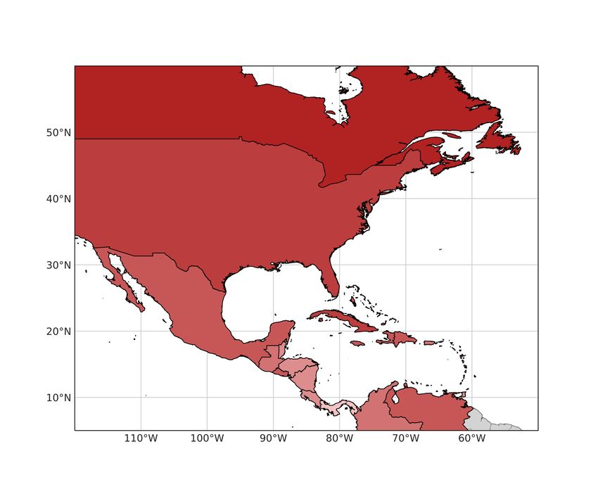
1 Introduction
Tropical cyclones (TC) are among the most devastating and deadliest natural hazards, causing
enormous damage and losses in almost all tropical regions. One of the most prominent examples
was Hurricane Katrina which made landfall (LF) on the US Gulf Coast close to New Orleans
in late August 2005. The accompanying rainfalls and storm surge caused by Katrina lead to the
flooding of 80 percent of the city of New Orleans. Overall, Katrina claimed 1800 lives and with
damages around $160 billion was the costliest natural disaster in US history (Britannica, 2021).
A new record in overall damages due to TCs was reached in 2017 when hurricanes Harvey,
Irma and Maria made landfall within a span of only four weeks leading to overall losses around
$220 billion (Munich RE, 2017). With their large impacts upon landfall, it is important to have
a good understanding of the disaster risk associated with tropical cyclones. This knowledge can
help decision makers to take necessary mitigation measures. Furthermore, (re)insurance
companies are interested in reliable probability distributions to build their portfolios correctly.

Tropical cyclones are relatively rare with globally around 90 storms in a year. With reliable
data only available for the last few decades the risk assessment of TCs is challenging
(Bloemendaal et al., 2020). Especially for extreme impact events with high return periods and
low probabilities the available data is sparse and therefore complicating reliable risk
assessment. When modelling disaster risk based solely on past events, extreme events can easily
be underestimated, due to their low frequency of occurrence. Information on such extreme
events is crucial, especially when assessing the vulnerabilities of communities and planning
necessary mitigation measures. Therein, lies the danger of catastrophes occurring that were not
within the modelled risk horizon (Woo, 2019). To better attribute for the described outcome
bias, Gordon Woo in 2016 first introduced the concept of using downward counterfactual (CF)
risk analysis to detect possible high impact events. By incorporating information on near miss
events the risk assessment at the tail of the distribution can be improved (Woo, 2016).
The term counterfactual is more commonly used in cognitive psychology, which defines a
downward counterfactual as a “thought about the past where the outcome was worse than what
actually happened” (Woo, 2019). Woo (2019) suggests that instead of treating history as fixed,
we can view it as one of many possible unfolding of past events. More common in risk analysis
are upward counterfactuals, meaning thoughts about past events imagining a better outcome.
This comes into play, for example, when analyzing how a past event could have been prevented
or how its damages and losses could have been minimized.
In order to detect possible high impact events by using counterfactual risk analysis, researchers
may consider how past events could have been worse if the circumstances were only slightly
different (Woo, 2019). As such, counterfactuals are defined as physically plausible unfolding
of past events illustrating a different but possible outcome. For tropical cyclones, this could
mean analyzing how a past hazard event could possibly have developed considering, for
example, higher wind speed on landfall, more precipitation, or stronger storm surges. Very
important for the risk analysis of tropical cyclones is also their trajectory. Only slight alterations
can determine whether a TC makes landfall or not or whether a community or city is hit by a
TC or not.

                                                                                                    6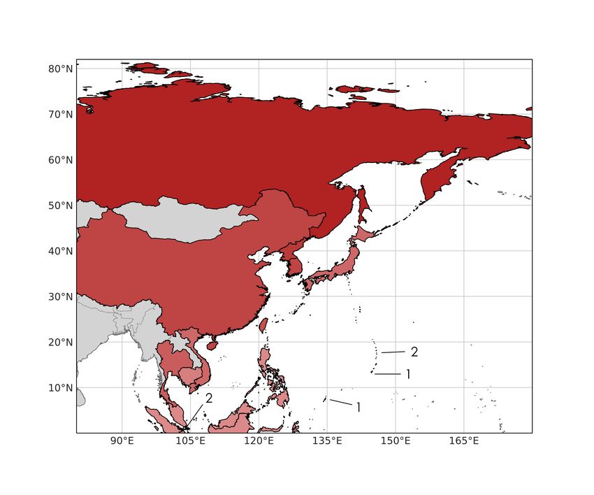
As an example, one can look at Hurricane Ivan, which headed towards New Orleans in 2004 as
a category 4 TC with wind speed of 225 km h-1 (Woo, Maynard and Seria, 2017). Luckily, the
hurricane turned east and did not directly hit New Orleans, making landfall instead east of
Mobile Bay, Alabama. Despite this given outcome previous forecast data of Hurricane Ivan
showed the storm possibly striking New Orleans. Considering this preceding forecast data, the
stochastic models indicated an entirely different loss distribution due to changes in the track
geometry, the hurricane intensity on landfall, the height of the storm surge, and the consequent
inland flood potential. The tail of this counterfactual loss distribution would have included the
loss realized one year later by Hurricane Katrina.
This example of Hurricane Ivan already illustrates the potential of forecasting data as a possible
source for counterfactual in risk analysis of TCs. Considering the chaotic nature of atmospheric
dynamics only slight perturbations can lead to a completely different path and evolution of the
storm. It is these small perturbations who decide which of the forecasted paths it follows closest
to. However, at some point in time each forecasted path can be viewed as a possible outcome
of the event. In this sense forecasting data of past events illustrate alternative, but physically
plausible outcomes. As such, forecasting data is a good source for counterfactual information
to expand the sparse observational data of TCs.

Building on the proposition of Woo (2016) there have been a few studies implementing
downward counterfactuals in their risk analysis (e.g., Aspinall and Woo, 2019; Oughton et al.,
2019). Up to date, no studies specifically used counterfactual data in the risk analysis of tropical
cyclones. Considering the challenges in TC risk analysis leading to an outcome bias towards
past events, and a possible underestimation at the tail of the hazard risk distribution, including
counterfactual data might be a powerful source in expanding the horizon of possible extreme
events. The aim of this thesis is therefore to explore forecast data as source for counterfactual
information of past TCs to expand the sparse observational data on which current risk analysis
is based. Thus, the data basis for risk analysis can be augmented significantly. This is illustrated
for the North Atlantic in Figure 1.1, where the density and amount of forecast tracks is much
higher than by merely considering observed tracks.
More specific, this thesis compares past yearly landfall rates, or landfall counts, of TCs to
counterfactual landfall rates based upon the combination of different forecast tracks of past TC
events. By specifically looking for downward counterfactuals the goal is to detect possible
extreme landfall rates. High or extreme landfall rates mark very stormy TC seasons in which
the cumulated damages and losses might be hazardous. This illustrated the year 2017 with three
landfalling TCs leading to the costliest year in TC damages. Thus, an exploration of how many
landfalls within a year could be expected when including downward counterfactuals in the risk
analysis can be of high importance for decision makers both regarding mitigation measures as
well as in the (re)insurance sector.

The dataset on forecast data used in this thesis contains global TC data from 2008 to 2019 with
several forecasts for each TC. Each forecast contains several forecast ensemble members,
representing an alternative path to the observed TC. Considering all TCs in this time period,
each combination of the individual forecast members corresponding to observed TCs can be

                                                                                                  7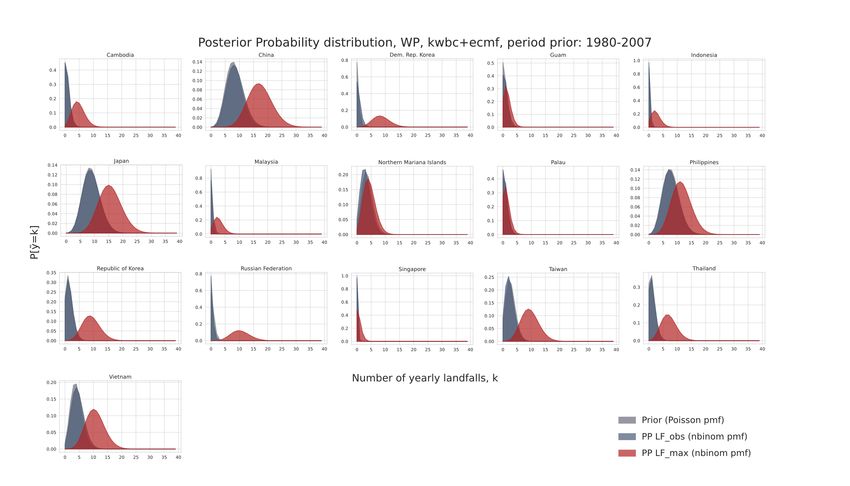
viewed as a counterfactual history or a counterfactual scenario. The resulting landfall rates of
said counterfactual scenario are then the basis to assess change in expected landfall rates.

Figure 1.1: All observed TC tracks in the North Atlantic for 2008-2019 (left) compared to all forecast tracks of the same
period (right).

Expected mean landfall rates, future landfall rates and extreme landfall rates based on
counterfactuals are analyzed using Bayesian inference (BI). The advantage of Bayesian
inference compared to the traditional frequentist statistical inference is that it incorporates the
notion of learning from new information. As such previous knowledge or data on TC landfall
rates can be included updated using observed or counterfactual landfall rates. Bayesian
inference then allows to make projections for future landfall rates. Also, Bayesian inference
returns probabilities that incorporate the uncertainty associated with the unknown variable of
interest (Gelman et al., 2020). As such, the probability of all possible values for mean or
extreme landfall rates can be explored and compared between counterfactual and observed
scenarios.
The previous knowledge of TC landfall rates incorporated in the analysis is based on observed
yearly landfall rates up to 2007. This represents the period before forecast data as
counterfactuals are available. The sensitivity of the BI towards this previous or prior
information is tested by comparing different periods of historic landfall. Thus, the period 1950
– 2007 is compared to the period 1980 – 2007. Further, the sensitivity of the BI is also tested
towards the used counterfactual information. The range of counterfactual scenarios is compared
across forecast data from two different providers and a combination of both.
The Bayesian inference analysis was conducted separately for six ocean basins North Atlantic
(NA), East Pacific (EP), West Pacific (WP), North Indian Ocean (NI), South Indian Ocean (SI),
and South Pacific (SP) (Figure 1.2). It was conducted for the ocean basins as well for the
individual countries within the respective basin.
When assuming a possible underestimation of extreme hazard events, it is of special interest to
analyze whether future projections of TC tracks based on counterfactuals are more extreme,
than historic data suggests. So, while several counterfactual scenarios are created and included
in the analysis the focus of the thesis are downward counterfactual scenarios and how they
change the risk assessment of yearly landfall rates of TCs. Overall, the following, interlinked,
research questions are answered:

    -     Can forecast tracks be used as a source for counterfactual information in risk analysis
          of tropical cyclones?

                                                                                                                            8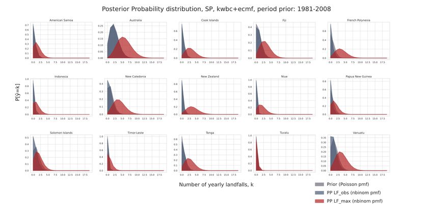
-    To what extent does accounting for downward counterfactual scenarios change the
         probability distribution of yearly landfall rates and future projections of yearly landfall?

    -    What are differences and similarities of findings across case studies for different
         … periods for prior information on landfall rates?
         … forecast dataset based on providing agency?
         … basins and countries?

Figure 1.2: Overview tropical cyclone basins and observed TC tracks 1980-2019. Arrows indicate general movement. NA:
North Atlantic, EP: East Pacific, WP: West Pacific, NI: North Indian Ocean, SI: South Indian Ocean, SP: South Pacific.

First in a background chapter risk of tropical cyclones and forecast data as source for
counterfactual risk analysis of tropical cyclones are explored more thoroughly. After, the
application of Bayesian inference within this thesis is presented, followed by a description of
the data. In Chapter 4 the results for the different case studies are presented, compared, and
discussed. Finally, in Chapter 5 follows the conclusion of the analysis and an outlook for
counterfactual risk analysis of tropical cyclones.

2 Background

2.1 Tropical Cyclone Risk
Tropical cyclones are symmetric low-pressure systems that develop in the tropics and can reach
sizes between 100 to 4000 km (Lohmann, Lüönd and Mahrt, 2016). They are characterized by
a mostly cloudless eye of a diameter between 8 and 200 km. The eye is surrounded with the
eyewall where convection and thunderstorm activity are strongest and underneath which the
highest near surface wind speeds can be found. This is the most dangerous and destructive part
of the TC. Spiraling outward from the eye there are often secondary cells arranged in bands.
They are called rainbands. The major basins of tropical cyclone formation are the North
Atlantic, East Pacific, West Pacific, North Indian Ocean, South Indian Ocean, and South Pacific
(Figure 1.2). The largest and the most TCs occur in the West Pacific. Depending on their region
of occurrence TCs are also called hurricanes, typhoons, severe tropical cyclones, tropical
cyclones, or severe cyclonic storms.
                                                                                              9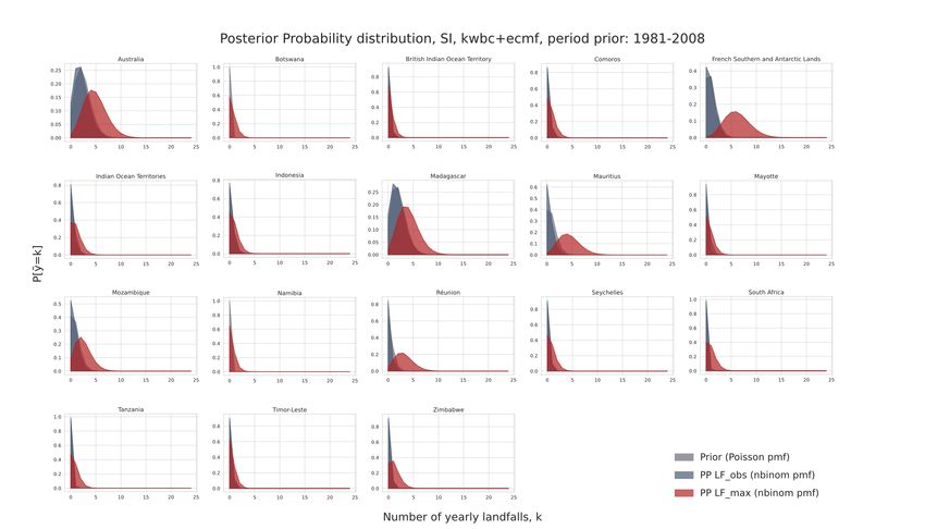
The main driver of TCs is latent heat release as air driven over warm waters humifies, rises and
the water condenses. When approaching land, they often intensify, due to the warm shallow
water, reaching maximum intensity at landfall. Cut off from their main energy source they will
weaken and dissipate over land also due to added friction at the surface.
The path a storm takes is referred to as the TC track. It marks the location of the center of the
storm, or the point of lowest pressure (central pressure) at different time steps. Landfall occurs
when all or parts of the eyewall passes across the coast. Accounting for the radius of the eyewall
within this thesis landfall is assumed when the track crosses the coastline or comes within 50
km of the coast.
TCs are categorized by their intensity measured as maximum sustained wind speed over 1
minute at 10 meters above ground. Most often used is the Saffir-Simpson scale (Table 2.1)
(Lohmann, Lüönd and Mahrt, 2016). The most severe category 5 refers to TCs with wind speeds
exceeding 250 km h-1. For extremely severe TCs maximum sustained winds above 300 km h-1
can be measured. When a storm develops the intensity of a tropical storm (sustained wind speed
higher than 33 kt) it is given a name to distinguish it easily from other cyclonic systems.
Table 2.1: Categorization of tropical cyclone. Based on Saffir-Simpson scale (adapted from NOAA, National Hurricane
Center and Central Pacific Hurricane Center, 2021; Wikipedia, 2021). Storm surge height and minimum pressure are for
reference only. Categorization is based on wind speed.

                                                                            Storm           Minimum
      Name           Category              Sustained winds
                                                                          surge (m)       pressure (hPa)
    Tropical
                          -1            ≤ 33 kt (≤ 62 km h-1)                  0
   Depression
 Tropical Storm           0           34-63 kt (63-118 km h-1)               0-0.9

     Tropical             1          64-82 kt (119-153 km h-1)              1.0-1.7           980-994

                                                                                                                       Named storms
     Cyclone              2          83-95 kt (154-177 km h-1)              1.8-2.6           965-979

                          3         96-112 kt (178-208 km h-1)              2.7-3.8           945-964
     (Major)
     Tropical             4         113-136 kt (209-251 km h-1)             3.9-5.6           920-944
     Cyclone
                          5           ≥ 137 kt (≥ 252 km h-1)                ≥ 5.7              ≤920

Damages due to tropical cyclones are caused by high wind speeds, storm surges, heavy rain and
spawning tornado activity (Zehnder, 2021). Strong sustained winds and wind gusts can cause
catastrophic damages to e.g., house, trees, and electricity infrastructure. Already a TC of
category 1 can cause damage to roofs, shingles, and gutters while a TC of category 5 will
destroy a high percentage of framed houses with total roof failure and wall collapse. However,
large amounts of the damage are often due to accompanying storm surges which are also
responsible for most of the deaths attributed to landfalling TCs.
The risk associated with natural hazards such as TCs can be understood as an interaction of
hazard, vulnerability and exposure (IPCC, 2014). The hazard itself is a combination of the
probability of the hazard occurring and its intensity. The analysis of TC landfall rates within
this thesis mostly concerns the probability component when assessing TC hazard risk.

                                                                                                                            10
The main challenge in correctly assessing the hazard component associated with TC risk is the
short historical data record which is not sufficient to calculate risk of extreme events with high
return periods. For example, to calculate the risk of a 200-year event a data record of at least
10,000 years would be necessary. Contemporary TC hazard risk analysis mostly relies on
catastrophe models that expand the short data records with a suite of thousands stochastic
events. Stochastic events are simulated, physically realistic storm tracks that are created by
statistically extrapolating historical records of past storms (Philip et al., 2019). While they
include some statistically added fluctuations, their characteristics and parameters are largely
similar to past observed events. This is due to the fact, that statistical models strongly rely on
distribution of past observations while the underlying parameters generating those observations
and the associated uncertainties are unknown (Woo, Maynard and Seria, 2017). This can lead
to a systematic underestimation of TC probabilities which is also illustrated by ever more
records being set within the last few years. Only recently a very active storm season in the North
Atlantic with 30 named storms developing in 2020 kept everyone uneasy (Bertogg, 2021).
2.2 Tropical Cyclone Forecast Data as Counterfactuals
Within the last few decades prediction of TC tracks has improved remarkably due to progress
in research and development of numerical weather prediction (Yamaguchi, Nakazawa and
Hoshino, 2012). Since around 1990, multilevel global and regional dynamical models have
become increasingly more accurate and replaced statistical or statistical dynamical models
(Rappaport et al., 2009). Keys in this advancement were better assimilation of satellite data,
improved model physics and higher model resolution. Another improvement in TC track
predictions is due to the implementation of the ensemble prediction system. Instead of making
a single forecast a set, or ensemble of forecast is produced to indicate the range of possible
future states of the atmosphere. Ensemble TC track predictions perform better on average and
are able to capture observed tracks that single deterministic predictions may miss.
For each TC several forecasts containing several ensemble tracks are produced. This is a ready
to use data base containing possible alternative track outcomes for past TCs. They are based
upon the dynamic situation at several points in the development of the TC and account for slight
differences in the atmospheric conditions. Compared to stochastically simulated TC tracks they
are less biased towards the outcome of past events. Their range and distribution concerning TC
variables are not guided by the same underlying assumptions about the distribution that is based
in a short historical record.
At each timestep the spread of the forecast members changes. Early storm forecasts will deviate
stronger from the observed track record while forecast from later stages, e.g., closer to landfall,
will more likely encompass the observed path of a storm. In this sense the probability of a
forecast member representing the actual outcome changes with lead time. This is important
when assessing the quality of forecasts. However, in counterfactual risk analysis the probability
of occurrence associated with individual ensemble members is of less importance. The focus is
rather how the observed TC could have turned out if the conditions were only slightly different.
In that sense one can argue that each forecast member, independent on lead time, is a plausible
alternative outcome of a past event, or a counterfactual.
113 Methods and Data
To investigate alternative outcomes of past tropical cyclones, existing forecast data is used as
source for counterfactual information. Bayesian statistical methods are applied to understand
how the landfall distribution based upon forecast data changes from a distribution using only
observed track data.
The analysis is conducted for all six major TC basins. For each basin probability distribution
of yearly landfall rates are analyzed aggregated across the basin as well as for each impacted
country of the region individually. As the EP mainly is of interest for the USA, in this case the
different US states are analyzed individually.
3.1 Methods
Statistical inference is concerned with learning something about a population based on data
sampled from the population (The CTHAEH, 2016). The main goals are estimation of unknown
parameters and data prediction. Bayesian inference is to model a set of data with a distribution
depending on unknown parameters. It relies on Bayes’ Theorem which relates the probability
of a parameter given the available data or observations to the model of the observations. The
understanding of probability in Bayesian inference is rooted in terms of physical tendencies and
degrees of beliefs rather than just the long-term frequencies on which frequentist inference is
based on. Thus, probability can be seen as a measure of belief of a certain event occurring. The
shape of the distribution expresses the belief as well as the attributed uncertainties for the belief
in possible parameter values.
3.1.1 Bayesian Inference of TC Landfall Rates
This thesis models yearly landfall rates of TCs on observed landfall rates or counterfactual
landfall rates based on forecast data. Yearly landfall rates can be represented as simple count
data and thus be modelled as a Poisson random variable (Elsner and Bossak, 2001). We assume
that observed yearly landfall (!) follows a Poisson mass distribution
y~??="(λ) (3.1)
The probability of an observation ! is
λ6 A 78
$(!|&) = , C=D ! = 0,1,2, … (3.2)
!!
λ is called a parameter, or rate, of the distribution controlling the distribution’s shape. It can be
any positive real number. ! on the other hand, must be a non-negative integer. A useful property
of the Poisson mass distribution is that its expected value is equal to its parameter, i.e.:
- [!|&] = & (3.3)
meaning λ represents the average number of yearly landfalls or mean landfall rates. With λ
being the single parameter governing the distribution of yearly landfalls the Bayesian inference
analysis is defined by modelling the belief in &. While the value of & is unknown, Bayesian
inference attributes a probability function to it based upon the knowledge and observations of
12yearly landfall rates. The goal is to arrive at a probability distribution representing the
probability of all possible values for the unknown parameter &. Put into Bayes’ formula it
follows
$(&)$(!|&)
$(&|!) = (3.4)
$(!)
which reads as the probability of the parameter & given the observations ! to the model $(!|&)
that we assume for the observations. $(&) is the prior distribution for & which represents the
initial guess or previous knowledge about the parameter. Bayesian inference is to update the
initial belief based on the available observations. The resulting probability distribution for & is
called the posterior distribution, $(&|!). The marginal distribution, $(!), is independent of the
parameter & which means it is a constant and can be omitted:
$(&|!) ∝ $(&)$(!|&) (3.5)
Prior
For a model using a Poisson distribution it can be shown analytically that the prior as well as
the posterior distribution of the parameter governing the process can be represented in a gamma
distribution (e.g. see Donovan and Mickey, 2019; Gelman et al., 2020). In Bayesian terms, the
gamma distribution is used as a conjugate prior for the Poisson distribution. The prior
distribution represents the belief in each possible value for & before introducing new
observations. Also, it expresses the model of the data to generate the posterior distribution,
$(&|!) (Donovan and Mickey, 2019). After deriving the likelihood $(!|λ), which is of the
form λ' A 7"8 , it follows, that the prior distribution must be in the form
$(λ) ∝ A 798 λ:7; = J4334(0, 2), (3.6)
which is a gamma density with hyperparameters 0 and 2 (Gelman et al., 2020). The gamma
distribution is a continuous probability distribution of the probability density function. The
hyperparameters are referred to as shape (0) and the rate (2). They are the guiding parameters
of the gamma distribution. As such they not only represent the previous knowledge about & but
they also express the uncertainties regarding the belief in $(λ) representing the true value of &.
They are related to & through the following formula:
0
&= (3.7)
2
Posterior
The gamma distribution is a conjugate distribution which can be updated with Poisson
distributed data. The resulting posterior distribution is also a gamma distribution with updated
hyperparameters. The effect of the new information or data used is then expressed in terms of
changes in parameter values (Donovan and Mickey, 2019). It follows the posterior distribution
$(&|!) ~ J4334(0 + "!L,< 2 + ") (3.8)
13where !* = (!; , … , != ) is a vector of independent and identically distributed observations. " is
the number of years observed. By modelling TC landfall rates in this manner, it is possible to
arrive at a posterior distribution mathematically.
Posterior Predictive (PP) Distribution
Based upon the posterior belief for λ, the next step is to predict future landfall rates, !+. While
observed landfall rates follow the distribution $(!|&), the true value for & is not known. To
account for the uncertainties, we average over all possible values of & to get a better idea of the
distribution of yearly landfall rates. The basic idea is to randomly sample possible values for &
from the gamma posterior distribution and then sample random values for yearly landfall rates
from a Poisson distribution based on the sampled value for &. Analytically it can be shown that
the resulting posterior predictive distribution follows a negative binomial distribution with the
following parameters (Gill, 2015):
1
!+~ MN O0 + "!P, Q (3.9)
"+2+1
3.1.2 Practical Calculations
Within this analysis the prior distribution is built by fitting a gamma distribution to observed
yearly landfall rates up to 2007. The observed mean landfall rates for this period, 6)*#+ , thus
represent the prior estimate for λ:
!>--?7= + !>--?7(=A;) , … + !>--?
6)*#+ = (3.10)
"
By choosing values for the hyperparameters shape (0) and the rate (2) it is expressed how high
the certainty is that 6)*#+ represents the true value of &. The hyperparameters are chosen in a
way that the relationship expressed in equation (3.7) is met:
:
- [&] = 6)*#+ = 9. (3.11)
Figure 3.1 illustrates how different values for the hyperparameters change the certainty for λ.
Narrow distributions imply a very high certainty for our belief in λ, while a broad distribution
implies high uncertainties for the mean landfall rates based solely on data up to 2007. Within
this analysis several values for scale and rate were tested but finally the parametrization of the
prior distribution was chosen as follows:
0 = 6)*#+ ∗ 2 and 2 = 4.
As the dark red curve in Figure 3.1 shows, these values express some confidence in previous
landfall rates while still expressing a rather high level of uncertainty acknowledging the fact
that the data used for the prior landfall rates is very short. Also, the data is influenced by
available data quality which differs among regions, time periods and providing agency. For the
analysis across basins, countries, and providers to be comparable the same values for 0 and 2
were used for all the analysis represented. It should be noted however, that is a strong
simplification, as one cannot assume that the uncertainty is the same for all regions, countries
14or time periods used for the calculation of 6)*#+ . However, this allows for a higher comparability
across case studies.
Figure 3.1: Gamma probability mass distribution depending on chosen hyperparameters. Illustrated based upon !!"#$ for the
NA using data from 1980 to 2007. For all analysis presented in this thesis the hyperparameters used are α=!!"#$ *β and β=4
(dark red line).
In a next step, the prior distribution is updated by incorporating new information of landfall
rates from 2008 to 2019. On one hand this is done using observed landfall rates as a reference
distribution. On the other hand, the posterior belief is updated with counterfactual landfall rates
based on forecast tracks. A scenario of counterfactual landfall rates represents one in many
possible combinations of all available forecast members. With the large number of forecast
tracks for each TC in the period 2008 to 2019 there can be as many posteriors built as there are
forecast track combinations.
The mean of the gamma posterior distribution represents the expected value for λ based upon
:A=6C! :A=6C
the added information, E[&|!] = 9A=
. The variance of the distribution is (9A=)!" . The posterior
distribution is denoted as $(λ|!!"# ) for the posterior belief based on observed landfall rates for
the period 2008-2019. The posterior belief based on the worst-case scenario with the highest
possible numbers of landfalls is denoted as $(&|!$%&'( ). The respective mean values of the
posterior distributions are E[&|!!"# ] and E[&|!$%&'( ].
The posterior predictive distribution based upon the observed or counterfactual landfall rates
portrays how future landfall rates, !+, would be expected given the respective scenario. Their
distributions for observed and worst-case scenarios are denoted as $(!+|!!"# ) and $(!+|!$%&'( )
respectively.
The negative binomial posterior predictive distribution has the same mean value as the posterior
:A =6C!
distribution, 9A=
. The variance however is greater for the posterior predictive distribution and
15:A =6C
defined as (9A=)"! (2 + " + 1). This is due to the additional uncertainty based on the fact, that
we are sampling new data values.
3.2 Data
For the Bayesian inference analysis of counterfactual information two datasets are necessary.
A dataset of observed TC tracks is necessary to build a prior knowledge or belief of past landfall
rates as well as the reference for the counterfactual scenarios. A dataset of TC forecast tracks
is used as a basis to build different counterfactual scenarios.
3.2.1 Observed Tropical Cyclone Data
The most complete set of tropical cyclone data available is the International Best Track Archive
for Climate Stewardship (IBTrACS) dataset from the National Oceanic and Atmospheric
Administration (NOAA) (Knapp et al., 2010). It contains a global collection of best-track data
combining data from different agencies worldwide. Best-track data of a tropical cyclone
contains the best estimate of storm position and intensity at intervals of 6 hours. If there is data
available from several agencies for one single event, the information is combined using
objective techniques that account for the differences between the international agencies (Knapp
et al., 2010).
As historic TC data this thesis uses data from the IBTrACS Project, Version 4 for the NA, EP,
WP, NI, SI and SP basin (Knapp et al., 2018). As the IBTrACS dataset is a collection of best-
track data rather than a reanalysis the data available is strongly influenced by methods used by
different agencies and time periods. For some regions the dataset contains TC data back to 1848
but global records spanning all basins only date back to 1945. TCs originally were mostly of
interest for shipping and only in the late 1950s and 1960s there was an increased interest in
their climatology and the risk they pose for coastal communities (Knapp, 2019). In the same
period routine aircraft observations were introduced, improving location estimates. Another big
improvement in TC reporting came with the incorporation of data provided by satellites. First
meteorological satellite observations in 1960s were merely able to identify systems from space.
However, with routine microwave imager satellites starting in the 1980s observations on rain
structure, expanse of winds, as well as the eye position improved considerably. Thus, TC data
from 1980 on is considered to be the modern era, as geostationary satellite coverage was nearly
global and global coverage from polar orbiting data was more widely available.
To account for this difference in data availability and quality and to gain more insight into the
sensitivity of the analysis on the prior information, two time periods are compared: 1950-2007
and 1980-2007. All BI analysis is carried out using prior information based upon the two
periods individually.
One problem when counting storms in IBTrACS is that the operational procedures when
including storms in TC reporting are dependent on the different agencies and may have changed
over time. For example, some agencies may include tropical depressions and sub-tropical
storms while others do not. To account for this fact, within this analysis only named tropical
cyclones are included. Not named storms are in general cyclones that never reach an intensity
higher than a tropical depression and therefore usually are not analyzed in much detail. Thus,
16by only including named storms some of the mentioned issues can be avoided. However, for
future analysis more detailed analysis of the included TCs might need to be considered (see e.g.
Schreck et al., 2014). Another, more practical reason for only including named storms is also
the problem of matching not named TCs across the different datasets of historic and forecast
data.
The IBTrACS dataset for the NA basin includes 1078 tracks within the period 1950 – 2019.
748 of those tracks are named tropical cyclones. For the other basins the numbers are similar
(see Table 3.1). An exception is the NI basin. For this basin named tracks only exist from 2005
onward. For this reason, the analysis of the NI basin includes all available tracks.
Table 3.1: Number of IBTrACS tracks and landfalls per basin and period.
NA EP WP NI* SI SP
all tracks 1078 1228 2040 608 1166 798
IBTrACS dataset named tracks 748 971 1728 55 845 514
1950-2019 landfalling tracks 462 334 1421 479 402 380
61.76% 34.40% 82.23% 78.78% 47.57% 73.93%
named tracks 571 749 1440 543 691 413
Prior period 1
landfalling tracks 360 245 1171 428 336 311
1950-2007
63.05% 32.71% 81.32% 78.82% 48.63% 75.30%
named tracks 318 484 701 137 549 366
Prior period 2
landfalling tracks 188 148 583 114 186 195
1980-2007
59.12% 30.58% 83.17% 83.21% 33.88% 53.28%
observation named tracks 177 222 288 65 154 101
period landfalling tracks 102 89 250 51 66 69
2008-2019 57.63% 40.09% 86.81% 78.46% 42.86% 68.32%
* As NI basin only has named tracks starting in 2005 all tracks are included for this basin.
For the analysis of the variable landfall only the positional information of latitude and longitude
is needed. Landfall occurs when the area of strongest wind i.e., the eyewall, crosses the
coastline or comes within 50 km of it. The variable used in the Bayesian Inference are yearly
landfall rates. Those are simple counts of tracks making landfall within each year and are
calculated for the entire basin as well for all relevant countries individually. Figure 3.2 gives an
overview over the yearly landfall rates of the entire dataset across the different basins.
As for the SI and SP the main TC season is in winter the landfall rates are not calculated yearly
but rather for the TC season. For both basins a TC season spans TC tracks from August of the
previous year until July of the indicated season year. Thus e.g., when mentioning the reference
period from 2008-2019 for the SI and SP basins this in fact refers to seasons 2009-2020
including data from August 2008 until July 2020.
17Figure 3.2: Bar chart of yearly number of named TCs (grey) and landfall rates (blue) for the individual basins. Red line
indicates the cut-off year or season for the data used to calculate the prior distribution (left of red line). Data on the right of
the red right are used to calculate the reference posterior distribution (observation period). *NI dataset also not named tracks
are included.
3.2.2 Forecasting Data and Counterfactual Scenarios
The forecast data used within this thesis is part of The Observing System Research and
Predictability Experiment (THORPEX) which is a big component of the World Weather
Research Programme under the World Meteorological Organization. The THORPEX
Interactive Grand Global Ensemble (TIGGE) was initiated in 2005 and contains among many
more forecasting data a dataset of tropical cyclone track data (Bougeault et al., 2010). This
dataset called TIGGE Model Tropical Cyclone Track Data (further simply referred to as TIGGE
dataset) holds model analysis and forecast data from several international meteorological
agencies. The dataset contains track data since 2008 and is updated daily (National Centers for
Environmental Prediction/National Weather Service/NOAA/U.S. Department of Commerce et
al., 2008).
For each TC event and provider there are several forecasts available, which in turn contain
several forecast members. Also, the number of available forecasts and members varies greatly
among TC events. The available forecast track variables depend upon the providing agency but
in general include name, time, position (latitude and longitude), minimum pressure, maximum
wind at 6-hourly intervals after the start of the forecast. Although there are TC forecast data
available from several agencies world-wide, only the data from two agencies span the entire
period from 2008-2019 without considerable data gaps. Thus, only data from the following
providers are used and compared in the data analysis:
- KWBC - National Centers for Environmental Prediction, National Weather Service,
NOAA, U.S. Department of Comerce and Meteorological Service of Canada,
Environment Canada
- ECMWF – European Centre for Medium-Range Weather Forecasts
18To be able to compare the different providers for each basin a set of counterfactual histories is
created based upon forecast members from the KWBC, the ECMWF or the combined dataset
using tracks from both providers. Table 3.2 gives an overview over the available number of
events and tracks within the TIGGE dataset. For example, the KWBC provides for the NA
basins 171,684 forecast tracks that span 432 storm events for the period between 2008 and
2019. To be able to create credible counterfactual landfall rates for the period 2008-2019, the
track data used must be comparable to the dataset of observed landfall rates in the same period.
Thus, only forecast tracks for named storms in the IBTrACS dataset were selected. Next to
named TC events the TIGGE dataset also contains forecasts for not named TCs as well for
invest tracks. Invest tracks are forecast for areas of disturbed weather, where possibly a TC
could develop and thus are monitored. After the selection according to named observed tracks
(IBTrACS), the number of NA tracks is reduced from 84,061 tracks (Table 3.2). To arrive at a
robust dataset several checks and corrections had to be implemented as described in the
following.
Table 3.2: TIGGE - Number of events and forecast tracks. The selected tracks show the sum of all forecast members across
the selected named TC events. The events are selected by name and cross-referenced with observed TC of the same period.
The difference of the selected and observed events indicates the number of missing events in the TIGGE dataset.
Number of Number Selected
Selected
Basin Provider TIGGE individual (observed)
tracks
events tracks events
ECMWF 314 110596 176 (177) 85337
NA
KWBC 432 171684 156 (177) 84061
ECMWF 417 126291 222 (222) 104472
EP
KWBC 516 185061 182 (222) 96258
ECMWF 333 169134 281 (288) 149901
WP
KWBC 681 237864 254 (288) 131631
ECMWF 64 17218 48 (65) 14162
NI
KWBC 104 23105 33 (65) 14899
ECMWF 374 128051* 153 (154) 62553
SI
KWBC 375 120251 144 (154) 68391
ECMWF 374 128051* 100 (101) 40657
SP
KWBC 229 75403 94 (101) 47506
* Within the data provided by the ECMWF tracks for the SI and SP basins are compiled in a single
dataset.
Treatment of TIGGE Data and Data Problems
The TIGGE database is a collection of forecast ensembles from different agencies. As such,
they make available data on TC forecast tracks as provided by the agencies and are not further
homogenized or otherwise quality controlled. This means that differences across basins, time
periods and providers are not accounted for. As within this thesis only the track or path is
relevant only the variables time and location are included. Systematic errors in track geometry
are difficult to detect and correct for. The biggest obstacle is, that a visual check of the track
information is unavoidable. However, looking at the sheer number of tracks which is overall
several hundred thousand tracks this cannot be done for each single track. Thus, there is no
thorough analysis or homogenization implemented in the presented analysis. However, some
19simple quality controls are conducted. Tracks meeting the following criteria are excluded from
the data analysis:
- duplicate tracks
- tracks with 2 or less timesteps
- tracks located out of bounds of basin
- tracks with unnatural changes in location between 2 timesteps (chance > 10°)
The tracks are grouped by event name and time to create individual events. For each named
event in the TIGGE dataset a visual check allows for correction of the following issues:
- reversed latitude
- wrong attribution of event name
Finally, the grouped dataset is cross referenced with the IBTrACS dataset to select all observed,
named, tracks within the period. The problem with this selection by name, is that possible
forecasts from an earlier stage of an event will not be included, as they are not yet named
correctly. For example, if an invest tracks later develops into a named storm not all forecasts
from earlier stages will be attributed with the later storm name. However, due to the large
number of events in the TIGGE dataset a correction of all not named or invest is not conducted.
Further, for most basins not for all observed events forecast tracks is available (see Table 3.2).
For some regions and periods there are gaps in the available data, especially in the earlier years
of the period. For example, for the years 2008 and 2009 there are several months of data missing
from the KWBC dataset. In the NA for example, out of the 177 IBTrACS events only for 156
events are forecast tracks available in the KWBC dataset. A much bigger gap exists for the NI
basin. As for this basin, also non-named tracks had to be included there are several events where
no forecasts are available.
To still be able to achieve a full set of events, the missing events in the TIGGE dataset were
replaced with the observed IBTrACS track. This means however, that for those events no
counterfactual tracks are available and only one outcome (landfall or no landfall) could be
considered.
Creating Counterfactual Scenarios
Landfall is calculated for the whole basins as well as for individual countries for each forecast
member. Counterfactual scenarios of landfall rates are created by sampling a forecast track for
each observed track in the period 2008 – 2019. The resulting yearly landfall rate represents one
possible counterfactual scenario of how the landfall could have been distributed within the
observed period. As with random sampling of the forecast tracks not the entire range of possible
counterfactual scenarios could be covered the counterfactual scenarios were created manually.
To this purpose, for each subset of individual provider and basin or country the probability of
an event making landfall is calculated based on the number of landfalling tracks compared to
the total number of forecast tracks:
20"V3WAD T4"UC4TT>"X C=DAY4?Z ZD4Y[?
$(T4"UC4TT) =
Z=Z4T C=DAY4?Z ZD4Y[?
With the thesis’ focus on downward counterfactuals the scenario of most interest is the worst-
case scenario. This scenario assumes landfall for an event if at least one of the forecast tracks
make landfall. Thus, all events with landfall probability higher than 0 were included. To then
build a range of possible counterfactual scenarios the events were sorted by their landfall
probability. For each new history the event with the lowest probability of landfall is assumed
to not make landfall. The final scenario represents the best-case scenario and assumes only
landfall for events where the probability of landfall is equal to 1, meaning all forecast tracks
make landfall.
This thesis focuses on exploring counterfactuals in terms of their range and focuses on what
extremes downward counterfactuals can reveal. Therefore, a further analysis of the probabilities
regarding a TC making landfall based on the percentage of landfalling forecast tracks is not
included in this thesis.
4 Results and Discussion
As described above, the Bayesian inference of yearly landfall rates are conducted for the
different …
… prior distributions based upon the period (1950-2007 vs 1980-2007),
… providing agencies of counterfactual data (forecast data from KWBC vs. ECMWF vs.
KWBC+ECMWF)
… basins and countries (NA, EP, WP, NI, SI, SP)
The focus of the results presented, is how the incorporation of counterfactual TC data change
our belief for yearly landfall rates in comparison to the same Bayesian Inference using observed
TC data.
For the individual basins and countries not all results across case studies are shown. For the
analysis across basins, an extended version, including results of each case study across prior
period and provider can be found in Appendix A.
4.1 Observed TC Landfall Rates
As seen in Figure 3.2, the data availability is not the same for all basins. For the NA and the
WP TC best-track data are available all the way back to 1950. For the SI, SP and EP however,
data is only reliably available since the 1960s. For the NI best-track data goes back to the 1950s,
but the dataset contains an abrupt shift in the number of TC events around 1980. This shift is
strongly informing the prior distribution, as the mean values for the two compared periods differ
by 3.3 landfalls a year (Table 4.1). However, for none of the other basins the differences in
mean values are bigger than 1. With such small differences the period used to form the prior
distribution does not have a great impact on the BI analysis. This is tested by updating the prior
probability by adding new observed landfall rates for the period 2008 to 2019. The right side
21You can also read