Improving crosshole ground-penetrating radar full-waveform inversion results by using progressively expanded bandwidths of the data
←
→
Page content transcription
If your browser does not render page correctly, please read the page content below
Near Surface Geophysics, 2021                                                                                        doi: 10.1002/nsg.12154

Improving crosshole ground-penetrating radar full-waveform inversion
results by using progressively expanded bandwidths of the data
Zhen Zhou1,2,3∗ , Anja Klotzsche1,2∗ and Harry Vereecken1,2
1 Agrosphere (IBG-3), Institute of Bio- and Geosciences, Forschungszentrum Jülich GmbH, Jülich, Germany, 2 Centre for High-Performance
Scientific Computing in Terrestrial Systems, HPSC TerrSys, Geoverbund ABC/J, Jülich, Germany, and 3 School of Information Engineering,
ZheJiang A&F University, Hangzhou, China

Received September 2020, revision accepted February 2021

                                                  ABSTRACT
                                                  In the last decade, time-domain crosshole ground-penetrating radar full-waveform in-
                                                  version has been applied to several different test sites and has improved the resolution
                                                  and reconstruction of subsurface properties. The full-waveform inversion requires
                                                  several diligent executed pre-processing steps to guarantee a successful inversion and
                                                  to minimize the risk of being trapped in a local minimum. Thereby, one important
                                                  aspect is the starting models of the full-waveform inversion. Generally, adequate start-
                                                  ing models need to fulfil the half-wavelength criterion, which means that the modelled
                                                  data based on the starting models need to be within half of the wavelength of the mea-
                                                  sured data in the entire investigation area. Ray-based approaches can provide such
                                                  starting models, but in the presence of high contrast layers, such results do not always
                                                  fulfil this criterion and need to be improved and updated. Therefore, precise and de-
                                                  tailed data processing and a good understanding of experimental ground-penetrating
                                                  radar data are necessary to avoid erroneous full-waveform inversion results. Here, we
                                                  introduce a new approach, which improves the starting model problem and is able to
                                                  enhance the reconstruction of the subsurface medium properties. The new approach
                                                  tames the non-linearity issue caused by high contrast complex media, by applying
                                                  bandpass filters with different passband ranges during the inversion to the modelled
                                                  and measured ground-penetrating radar data. Thereby, these bandpass filters are con-
                                                  sidered for a certain number of iterations and are progressively expanded to the se-
                                                  lected maximum frequency bandwidth. The resulting permittivity full-waveform in-
                                                  version model is applied to update the effective source wavelet and is used as an
                                                  updated starting model in the full-waveform inversion with the full bandwidth data.
                                                  This full-waveform inversion is able to enhance the reconstruction of the permittivity
                                                  and electrical conductivity results in contrast to the standard full-waveform inversion
                                                  results. The new approach has been applied and tested on two synthetic case studies
                                                  and an experimental data set. The field data were additionally compared with cone
                                                  penetration test data for validation.

                                                  Key words: 2D, Data processing, Ground-penetrating radar, Inversion.

∗ E-mails:   z.zhou@fz-juelich.de and a.klotzsche@fz-juelich.de

© 2021 The Authors. Near Surface Geophysics published by John Wiley & Sons Ltd on behalf of European Association of                        1
Geoscientists and Engineers.
This is an open access article under the terms of the CreativeCommonsAttribution License, which permits use, distribution and reproduction in
any medium, provided the original work is properly cited.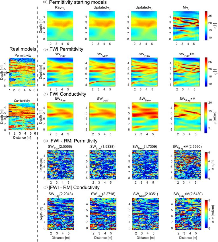
2 Z. Zhou, A. Klotzsche and H. Vereecken

I N T RO D U C T I O N                                               of soil water content (e.g., Looms et al., 2008; Kuroda et al.,
                                                                     2009). The good consistency illustrates crosshole GPR is able
Detailed and high-resolution characterization of variable sat-       to close the gap between small-scale investigations with high-
urated soil-aquifer systems is critical and full of challenges,      resolution (e.g., coring) and large-scale zones mapping (e.g.,
but highly important to improve the understandings of flow           flowmeter tests).
and transport processes of subsurface water. Small-scale soil              Traditionally, ray-based approaches based on the geomet-
heterogeneities can have a significant influence on the plant        rical ray theory are used for crosshole GPR data to derive
water uptake process, the transport process of pollutants or         tomographic images of the subsurface, which exploit first-
greenhouse gas emissions from peatland and permafrost soils          arrival travel times and maximum first-circle amplitudes of
(e.g., Simmer et al., 2015; Vereecken et al., 2016; Klotzsche        the GPR wave (e.g., Maurer et al., 2004; Dafflon et al., 2012).
et al., 2019a). In addition, the precision of large-scale atmo-      For such approaches, damping and smoothing constraints are
spheric models is influenced by recharging and transport of          necessary to stabilize the inversion (e.g., Holliger et al., 2001;
subsurface water (Becker, 2006). To enhance our understand-          Maurer and Musil, 2004). Thereby, most applications con-
ings of such processes, high-resolution images and accurately        sider only a limited angular coverage of the rays to avoid an
described subsurface properties, especially for small-scale het-     increasing apparent velocity for increasing ray path angles (Pe-
erogeneities of aquifers, are highly important (e.g., Klotzsche      terson, 2001). Ray-based approaches are often not able to re-
et al., 2019b). Thereby, some key parameters of geophysical          solve targets smaller than the dominant wavelength and rel-
and hydrological investigations, such as relative dielectric per-    atively smooth images are obtained, with a resolution that
mittivity, electrical conductivity, hydraulic conductivity and       scales approximately with the diameter of the first Fresnel
porosity, play an important role (e.g., Binley et al., 2015).        zone. In comparison to ray-based approaches, full-waveform
Traditional approaches to characterize aquifer properties ei-        inversion (FWI) exploits the entire information of the data (or
ther capture a small spatial sampling with a high vertical but       significant parts of it), and is therefore able to provide higher
poor lateral resolution, such as drillings and core sampling         resolution images within the sub-wavelength scale. Inspired
(Tillmann et al., 2008), or, have an average response over a         by the FWI approach that was first developed and applied in
large volume with a lack of detailed characterization at smaller     the seismic community (e.g., Tarantola, 1984; Shin and Cha,
scale, such as pumping test and remote sensing methods (Lan-         2008; Virieux and Operto, 2009), a 2D time-domain FWI for
don et al., 2001). In the last decades, geophysical methods          crosshole GPR data was implemented by Ernst et al. (2007a,
have been developed and applied to obtain images of the near         b) and Kuroda et al. (2007), based on solving Maxwell’s equa-
subsurface and to improve the characterization of hydrogeo-          tions. Meles et al. (2010) improved the method of Ernst et al.
logical properties (Binley et al., 2015), such as seismics (e.g.,    (2007a) by including the vector characteristics of the EM
Doetsch et al., 2010), electrical resistivity tomography (ERT;       fields, and introduced a simultaneous update of the permit-
e.g., Coscia et al., 2011) and ground-penetrating radar (GPR;        tivity and electrical conductivity parameters. Klotzsche et al.
e.g., Klotzsche et al., 2018). Especially, crosshole GPR has         (2019b) provides an overview of the current developments,
shown a great potential to characterize aquifers and has ma-         applications and corresponding challenges for the 2D cross-
tured because of the opportunity to derive the highest possi-        hole time-domain GPR FWI. Several applications of the FWI
ble resolution by using high-frequency electromagnetic (EM)          to crosshole data sets from different environments, ranging
pulses (e.g., Paz et al., 2017), and the opportunity to simul-       from various aquifers to karst environments, demonstrated
taneously derive electromagnetic wave velocities and ampli-          that the FWI was able to provide higher resolution images
tudes. The estimated EM velocities and attenuations can be           than the ray-based approaches, and provided images within
transformed into relative dielectric permittivity εr and elec-       decimetre scale.
trical conductivity σ (e.g., Ernst et al., 2007b; Dafflon et al.,          Generally, FWI approaches can be implemented in the
2011), which are related for example to water and clay con-          time and frequency domains. Both methods have pros and
tent, respectively (e.g., Kowalsky et al., 2005; Cassidy, 2007;      cons. While frequency approaches can highly minimize the
Klotzsche et al., 2014). For crosshole applications, the EM          calculation costs and improve the cycle skipping problem, the
pulses are emitted from a dipole-type antenna in a borehole          time-domain approaches provide the most flexible framework
and received by an antenna in another borehole. Within the           to apply time windowing of arbitrary geometries (Virieux
scope of hydrogeological site characterization, several stud-        and Operto, 2009). Similar to seismics, frequency-domain
ies have shown the potential of crosshole GPR by compar-             FWI approaches for GPR data have also been implemented.
ing GPR permittivity results with independent measurements           Such approaches allow, for example, to use only a few

                  © 2021 The Authors. Near Surface Geophysics published by John Wiley & Sons Ltd on behalf of European Association of
                                                                           Geoscientists and Engineers., Near Surface Geophysics, 1–23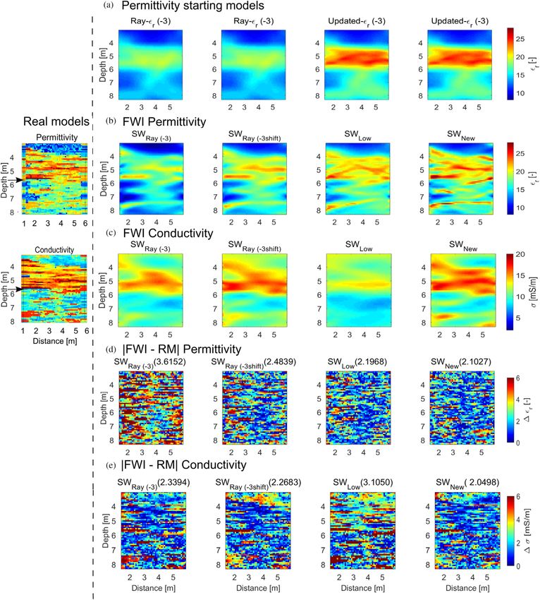
Improving crosshole ground-penetrating radar full-waveform inversion results 3

discrete frequencies of the data and allow the possibility to        mic inversion. For example, the frequency hopping method
implement a wider range of misfit functions, which are benefi-       was used in frequency domain for microwave applications
cial for frequency-dependent medium properties (e.g., Lavoué         (Chew and Lin, 1995; Dubois et al., 2009) and for seismic
et al., 2014). Ellefsen et al. (2011) inverted measured crosshole    data (Pratt et al., 1998; Maurer et al., 2009). Thereby, the
GPR data from a laboratory tank by using a 2.5D frequency-           inversion is first performed with a low-frequency bandwidth.
domain FWI approach. Furthermore, a 2D frequency-domain              The results of this low-frequency inversion are then used as
quasi-Newton approach for multioffset GPR data was imple-            the next starting models for the FWI, with a progressively
mented and tested on a synthetic model (Lavoué et al., 2014),        increased frequency bandwidth. These steps are repeated until
and on GPR data acquired at carbonate rocks (Pinard et al.,          the maximum boundary of the frequency bandwidth reaches
2016). Although frequency-domain FWI seems to have certain           the centre frequency of the data. One problem of this approach
benefits compared with time-domain FWI, for most experi-             is that, for many field experimental data sets, not enough low-
mental GPR data, low-frequency data are missing or show a            frequency data are present or that the low-frequency data are
low signal-to-noise ratio. Until now, almost all successful ap-      highly contaminated with noise. Therefore, several researchers
plications to experimental data have been performed using the        tried to generate artificial low-frequency information for seis-
time-domain FWI approach for GPR data (Klotzsche et al.,             mic data, for example, by using mathematical transformations
2019b).                                                              based on the angle difference identity for cosine (e.g., Wang,
      The 2D time-domain crosshole GPR FWI uses a                    et al., 2019) or using the modulation signal approach intro-
conjugate-gradient algorithm (Polak et al., 1969) to minimize        duced by Wu et al. (2014). To tame the non-linearity issue
the misfit function between the measured and modelled data.          of GPR inversion, also for the time-domain FWI, Meles et al.
This minimization can be achieved by updating the model              (2012) presented an inversion scheme that incorporated a
parameters εr and σ by calculating updating directions and           frequency-dependent effective source wavelet. Thereby, the
corresponding step lengths for both parameters according to          modelled data are progressively bandwidth expanded (PBED)
the conjugate-gradient algorithm. It is well known that the          in an iterative process based on a stepwise increased frequency
non-linearity problem of the forward modelling is associated         bandwidth of the source wavelet, while the observed data
mainly with multiple scattering of propagating waves (Mora,          kept the full bandwidth. This approach worked very well for
1987; Meles et al., 2012). As with most of the inversion ap-         synthetic data, but for experimental data, the choice of the
proaches, the FWI with conjugate-gradient method is also ill         frequency bandwidths and the inversion parameters such as
posed, which means that we can have data residuals of mul-           the perturbation factors hindered a successful application so
tiple models which fit the data equally well (e.g., Backus and       far.
Gilbert, 1968; Brittan et al., 2013). In addition, the FWI re-             In this paper, we introduce a novel approach that contin-
sults can be trapped in local minima if certain criteria are not     ues the work of Meles et al. (2012), by improving the permit-
fulfilled. One of the most important criteria is that the for-       tivity starting model and the effective source wavelet, based
ward modelled data of the starting model are within half of          on progressively expanded bandwidths of the modelled and
a wavelength of the measured data in the entire inversion do-        observed data (PEBDD). In contrast to the approach of Meles
main. Normally, ray-based starting models fulfil this criterion      et al. (2012), we applied tapered bandpass filters to the ef-
(Virieux and Operto, 2009). However, in the presence of spe-         fective source wavelet (used for the modelled data) and the
cific subsurface structures such as high contrast layers related     observed data. The new FWI scheme can be divided into two
to, for example, the presence of the water table or small-scale      steps: (1) construction of the new permittivity starting model
heterogeneities, the ray-based starting models can be inaccu-        by using PEBDD and (2) performing the FWI with the new
rate and adaptations are required (e.g., Klotzsche et al., 2012      starting model and an updated effective source wavelet us-
and 2013). An experienced user and other tools, such as the          ing the full bandwidth data. To evaluate our new inversion
amplitude analysis approach, are needed to ensure that the           scheme, we performed two synthetic case studies. One study
measured data are fully understood before starting the FWI           is conducted using standard ray-based starting models and
and in the entire domain of interest the starting models ful-        the second considers an enforced smaller starting εr model,
fil the half-wavelength criterion (Klotzsche et al., 2014; Zhou      which provides modelled data more than half a wavelength
et al., 2020).                                                       away from the measured data. After the validation of this
      To solve the problem of being trapped in a local minimum       new approach, we used the crosshole GPR FWI with PEBDD
in the FWI, and to avoid a detailed pre-processing of the data,      scheme to characterize the Krauthausen test site, using four
some solutions were proposed in microwave imaging and seis-          inline crosshole GPR sections.

© 2021 The Authors. Near Surface Geophysics published by John Wiley & Sons Ltd on behalf of European Association of
Geoscientists and Engineers., Near Surface Geophysics, 1–23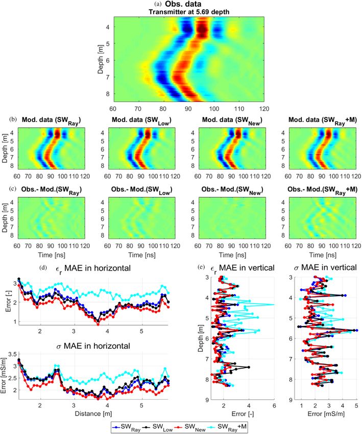
4 Z. Zhou, A. Klotzsche and H. Vereecken

METHODS                                                                          data Eobs and model-predicted data Esyn (ε, σ ):

Ground-penetrating radar full-waveform inversion                                             1     syn                         T
                                                                                C(ε, σ ) =                      E (ε, σ ) − Eobs
                                                                                             2 s r τ                                r,τ
Standard full-waveform inversion scheme

In this section, we only discuss the most important data pro-                                δ (x − xr , t − τ ) Esyn (ε, σ ) − Eobs ,            (3)
                                                                                                                                   r,τ
cessing and inversion steps of the standard full-waveform in-
                                                                                 where s, r and τ are transmitters, receivers and the observation
version (FWI) approach. For more detail, we refer the reader
                                                                                 time, respectively. T denotes the transpose operator. Each of
to Klotzsche et al. (2019b). One critical aspect to guarantee
                                                                                 the fields is locally defined at any point of space x and time
reliable and stable crosshole ground-penetrating radar (GPR)
                                                                                 t. The multiplication with the Dirac delta δ function selects
FWI results is to define adequate starting models. These start-
                                                                                 from the entire wavefield the used receiver locations and ob-
ing models should return modelled data that are within half a
                                                                                 servation times. Additionally, the gradients of the misfit func-
wavelength (λ/2) of the measured traces in the entire inversion
                                                                                 tion with respect to permittivity ∇Cε and conductivity ∇Cσ
domain to avoid cycle clipping and trapping of the inversion
                                                                                 are calculated by a zero-lag cross-correlation of the synthetic
in a local minimum of the misfit function (Meles et al., 2012).
                                                                                 wavefield with the back-propagated residual wavefield:
In addition, an effective source wavelet needs to be estimated,
because the source wavelet emitted into the earth system is                       ∇Cε (x )
unknown for experimental GPR data and accounts addition-
                                                                                            =   (δ(x − x )∂t Esyn )T GT RS
                                                                                  ∇Cσ (x )    s
ally for coupling effects. Such an effective source wavelet is
estimated with two steps. First, an initial source wavelet is                                           (δ(x − x )Esyn )T GT RS                  (4)
estimated using only horizontally travelling rays. The initial
                                                                                 with
wavelet only considers the shape of the wavelet and the am-

plitude is normalized to one. This initial wavelet is in a second                RS =            δ (x − xr, t − τ ) Esyn (ε, σ ) − Eobs
                                                                                                                                            r,τ
step updated using the deconvolution approach (e.g., Ernst                              r    τ

et al., 2007b; Klotzsche et al., 2010) in the frequency domain,                     =              [Esyn ]r,τ .                                   (5)
which can be described by:                                                              r    τ

                                     −1                                    where RS can be interpreted as the back-propagated residual
Ĝ       f       = Êsyn ( f ) ŝk f + ηD     ,                          (1)
                                                                                 wavefield in the same medium as the incident wavefield Esyn .
                                                                                 The spatial delta function δ (x − x ) in equation (4) corre-
         and                                                                     sponds to the spatial components of the gradients and reduces
                                −1                                       the inner product to a zero-lag cross-correlation in time (Meles
ŝk+1            f       = Ĝ f + ηI     Êobs f ,                       (2)     et al., 2010). Note that two different step-lengths are consid-
                                                                                 ered in the process of estimating how far the permittivity and
where sk represents the initial source wavelet. Esyn is the for-                 conductivity models need to be updated in the gradient di-
ward modelled data based on the ray-based starting models                        rection. The medium parameters are updated to reduce the
and sk . G is Green’s function and Eobs is the observed GPR                      misfit function equation (3) by updating all gradient values
data. ηD and ηI are prewhitening factors that are applied to                     in equations (4) and (5). In this paper, we employed the gra-
stabilize the solution and avoid dividing by zero. ˆ indicates                   dient normalization approach as proposed by van der Kruk
frequency domain. sk+1 describes the updated effective source                    et al. (2015) to minimize inversion artefacts close to the trans-
wavelet with an optimized phase and amplitude. If needed,                        mitter and receiver positions in the vicinity of the boreholes.
this wavelet can be updated after a certain number of FWI it-                    As stopping criterion for the inversion, we consider that the
erations. Note that for most experimental data applications,                     root-mean-squared (RMS) error between observed and mod-
the effective source wavelet is based on the ray-based models.                   elled data changes less than 0.5% between two subsequent
      The forward modelling is based on a 2D finite-difference                   iterations. Besides the stopping criterion, reliable FWI results
time-domain (FDTD) solution that solves Maxwell’s equa-                          also include the absence of a remaining gradient for the final
tions in the Cartesian coordinates (Ernst et al., 2007a; Meles                   models and a match between the measured and modelled data
et al., 2010). In the process of the inversion, the misfit function              with a correlation coefficient greater than 0.8 (e.g., Klotzsche
C (ε, σ ) is defined by the differences between the observed                     et al., 2019b). For synthetic case studies, the mean absolute

                              © 2021 The Authors. Near Surface Geophysics published by John Wiley & Sons Ltd on behalf of European Association of
                                                                                       Geoscientists and Engineers., Near Surface Geophysics, 1–23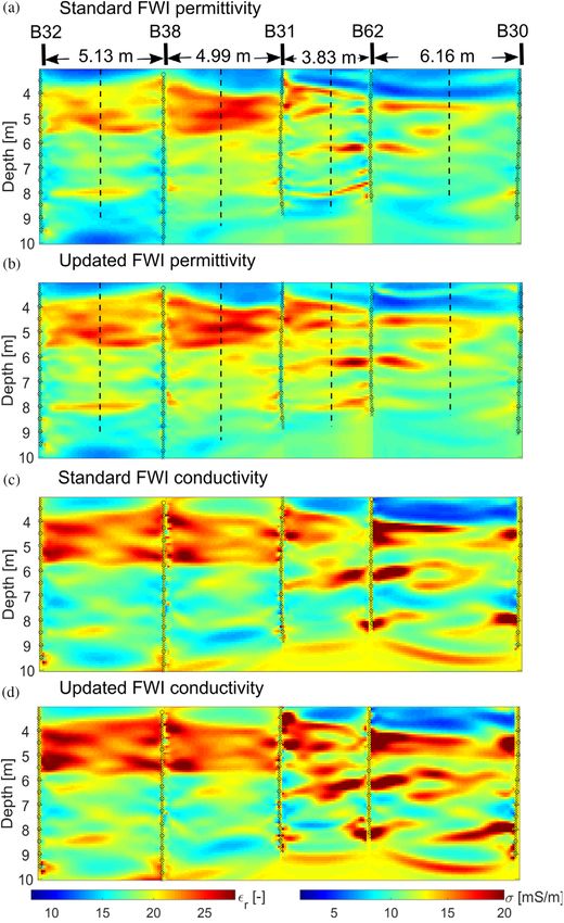
Improving crosshole ground-penetrating radar full-waveform inversion results 5

error (MAE) in the 2D domain can be described as (Zhou                 ing models for the FWI are based on the ray-based results
et al., 2021):                                                          ModelRay (‘Ray ( εr ) and Homo (σ )’ in Fig. 1b, green box).
                                                                       Traditionally, for the conductivity a homogeneous starting

         k
           m
MAE =              (|RMi, j − FWIi, j |)/(k × m),               (6)    model is used based on the results of the first cycle ampli-
         i=1 j=1                                                       tude inversion of the data (Klotzsche et al., 2019b). Using the
                                                                       starting models with the sub-source wavelet and sub-observed
where RMi, j and FWIi, j represent the input and the FWI model         data with the same smallest bandwidth, we perform a certain
value located at the cell of i, j. k and m show the number of          number of iterations of the FWI. Note that we chose for our
cells in the 2D domain along horizontal and vertical direc-            studies five iterations for each bandwidth expansion n (Fig. 1b,
tions, respectively.                                                   green box loop 1). Several synthetic tests indicated that this
                                                                       choice is the best compromise between computational effi-
                                                                       ciency and stability of the inversion. The perturbation fac-
Novel progressively expanded bandwidths of the modelled
                                                                       tors for the inversion, which are necessary to define the step-
and observed data full-waveform inversion scheme
                                                                       lengths for the gradient approach, are kept the same as for the
Different from the approach of Meles et al. (2012) that is us-         standard FWI. The εr and σ FWI results after this fifth iter-
ing the expanded bandwidths for the effective source wavelet           ation are considered as the next new starting models for the
only, we introduce a new scheme that applies the progres-              next sub-data with progressively expanded bandwidth, while
sive increase bandwidths on both measured data and effec-              the maximum cut frequency is increased by 4 MHz in our case
tive source wavelet. Our new updated approach proposes to              (Fig. 1b, green box loop 2). These steps are repeated until the
tame the non-linearity issue of the time-domain FWI, which             selected maximum cut frequency is reached (Fig. 1b green box
can be considered as an extension of the standard FWI pro-             loop 1: n = nmax ). Until this point all data (including source
cedure to improve the characterization of small-scale subsur-          wavelet and observed data) used for the inversion are progres-
face structures. Therefore, we apply the idea of a frequency-          sive bandwidth expanded.
domain approach that uses longer wavelengths with lower                     Third, the FWI with the full bandwidth data (FBD) is
frequencies in the beginning of the inversion to avoid the cy-         calculated (Fig. 1b, red box). From these results, only the
cle skipping problem and that defines the bandpass filters ac-         PEBDD permittivity FWI results with the maximum cut fre-
cording to the centre frequency of an effective source wavelet.        quency are considered as new permittivity starting model in
First, we construct a series of bandpass filters with different        the next step (see, ‘low-freq FWI ( εr )’ in Fig. 1b). Together
high cut frequencies, while keeping the low cut frequency con-         with the conductivity starting model, which is the same as
stant. Figure 1(a) shows an example for an effective source            for the traditional FWI (Fig. 1b, ‘Homo (σ )’), we construct
wavelet with a centre frequency of 65 MHz and a bandwidth              the new starting models ModelNew . Note that tests indicated
of 12–140 MHz. For such a wavelet, we would select a low               that using the conductivity results with the maximum cut fre-
cut frequency of 12 MHz, while the maximum cut frequency               quency as starting models does not improve the final results.
is considered larger than the centre frequency of the effective        The new starting models ModelNew and the traditional effec-
source wavelet, which in our case is 68 MHz. To smooth the             tive source wavelet SWRay are used in the next step to gener-
bandpass, we assigned two tapers with lengths of 12 MHz                ate an updated effective source wavelet SWLow with the full
and 10 MHz for the starting and ending frequency points,               bandwidth data using the deconvolution approach (equation
respectively (Fig. 1a). These tapered bandpass filters are ap-         (2), Fig. 1b, red box). After obtaining the updated source
plied in the next step to the observed GPR data and the ef-            wavelet SWLow , an updated FWI is performed with the new
fective source wavelet, which results after applying the FDTD          starting models ModelNew and the wavelet SWLow . Generally,
in sub-modelled data with a similar frequency spectrum as the          a second-updated source wavelet SWNew is necessary to fur-
sub-observed data (Fig. 1b, green box). The comparison of the          ther improve the FWI results. Thereby, the effective source
effective source wavelets with the expanded bandwidths with            wavelet SWLow is updated to SWNew using the deconvolution
the different bandpass filters shows a clear effect on the phase       method with the wavelet SWLow and the permittivity model
and amplitude of the wavelets (Fig. 2).                                from the updated FWI results with SWLow . The final updated
     Second, the FWI with the progressively expanded band-             FWI results with FBD are solved based on the second-updated
widths of the modelled data and observed data (PEBDD) is               source wavelet SWNew and the new starting models ModelNew
performed (Fig. 1b, green box loops 1 and 2). The first start-         (details can be found in Fig. 1b).

© 2021 The Authors. Near Surface Geophysics published by John Wiley & Sons Ltd on behalf of European Association of
Geoscientists and Engineers., Near Surface Geophysics, 1–23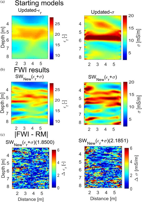
6 Z. Zhou, A. Klotzsche and H. Vereecken
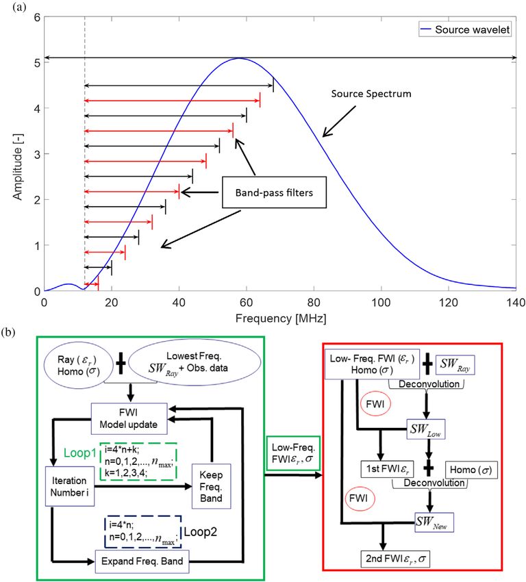
Figure 1 (a) Example for an effective source wavelet amplitude spectrum and corresponding stepwise increased bandpass filters (shown schemat-
ically by the black and red horizontal bars). These filters are progressively expanded after the centre frequency is reached and applied to the
observed data and the effective source wavelet. The bandpass filters start at the lowest frequency of 12 MHz (taper length 12 MHz) indicated
by a vertical dashed line. The high cut frequency is stepwise expanded every five iterations of the FWI and has a taper of 10 MHz. After the
highest corner frequency of 68 MHz is reached (centre frequency of 65 MHz), all subsequent iterations use the full bandwidth of an updated
source wavelet and the observed data. (b) Flow chart of the new proposed approach (adapted from Meles et al., 2012). In the first part (green
box) the progressively expanded effective source wavelet and the observed data are used, in which i, n and k represent all iterations using all
sub-data, the numbers of bandwidth expansions, and individual iterations of each group sub-data, respectively. nmax is depending on the centre
frequency of the effective source wavelet. In this case, we select nmax = 13. In the second part (red box), the full bandwidth data (FBD) FWI is
performed, where two effective source wavelet corrections are performed and used during FWI. The final result is indicated by the second FWI
with the SWNew as an effective source wavelet.
R E S U LT S A N D D I S C U S S I O N (GPR) FWI results, we construct realistic synthetic models of
relative dielectric permittivity and electrical conductivity using
Synthetic case studies
a stochastic simulation (sequential Gaussian simulation). For
Synthetic study I: Stochastic input models and ray-based start- the simulation, existing data set of the Krauthausen aquifer
ing models test site in Germany is used to generate a facies model with cer-
tain hydrological and geophysical parameters (based on Till-
To verify the aforementioned new full-waveform inversion
mann et al 2008, and more details can be found in Zhou et
(FWI) scheme for improving the ground-penetrating radar
al 2021). The construed aquifer consisted of a three-layered
© 2021 The Authors. Near Surface Geophysics published by John Wiley & Sons Ltd on behalf of European Association of
Geoscientists and Engineers., Near Surface Geophysics, 1–23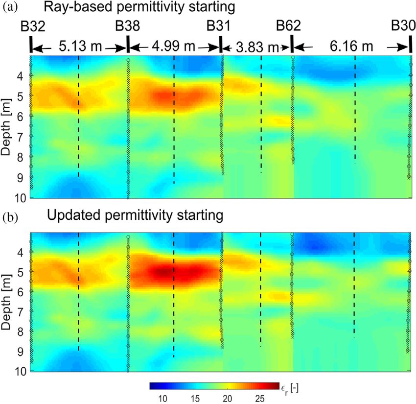
Improving crosshole ground-penetrating radar full-waveform inversion results 7

Figure 2 Comparisons of the selected sub-source wavelets with the different bandpass filters of the new PBEDD approach used for synthetic
case study I in time domain. (a) Shows the source wavelets with the absolute amplitudes and (b) the corresponding wavelets normalized to the
corresponding minimum (or maximum) for a better comparison of the phase.

Figure 3 Comparisons of the (a) effective source wavelets and the (b) corresponding frequency spectra of the different steps of the new PBEDD
approach used for synthetic case study I. The legend values in (b) indicate centre frequencies for different source wavelets. The source wavelet
used to generate the ‘observed data’ is indicated with a dashed black line. Note that SWNew ( εr + σ ) is the effective source wavelet based on the
results shown in the Appendix.

structure similar to the Krauthausen aquifer: sandy layer be-               neous models and used the results of the first cycle amplitude
tween 1.0 m and 4.0 m, sandy gravel between 4.0 m and 5.5                   inversion of the experimental data.
m and below coarse gravel (left side in Fig. 4 and Fig. 8). For                  To keep it as realistic as for experimental data applica-
the unsaturated zone above water table at 2.0 m, we chose                   tions, we used the ray-based starting models to estimate an ef-
a homogeneous layer with a relative permittivity of εr = 4.4                fective source wavelet (SWRay ; blue curves in Fig. 3a and b) and
(not shown, same for all following inversions). To generate the             performed the standard FWI (first column of Fig. 4b and c). As
realistic synthetic GPR data (called observed data), we used a              expected, the FWI results show higher resolution images as the
source wavelet (SWReal ; dashed curves in Fig. 3a and b) based              ray-based results within decimetre-scale resolution. Because of
on available experimental data from the cross-section B38-31                the known input models, we can calculate the mean absolute
of the Krauthausen test site (Gueting et al., 2015). Similar to             error (MAE) according to equation (6) between the resolved
the acquisition of experimental data, a semi-reciprocal acqui-              FWI models and the true input models based on the stochastic
sition set-up was used with transmitter and receiver spacing                simulation (shown in the first column titles of Fig. 4d and e).
of 0.5 m and 0.1 m, respectively. The realistic synthetic cross-            The final results were obtained after 28 iterations, and the in-
hole GPR data are modelled with the same time-domain 2D                     verted results fulfilled the criteria for a reliable inversion. The
FDTD approach as used for the FWI. Similar to experimental                  corresponding RMS curve that is calculated between the ob-
data applications, we defined the εr starting model for the                 served and modelled radar data is indicated by the blue curve
FWI by picking the first-arrival times of the synthetic data                in Fig. 5 with the final RMS of 6.9945 × 10⁻⁷ . Generally,
and performed a ray-based inversion (first column of Fig. 4a;               most of the distinct features of the stochastic input models are
e.g., Maurer and Musil, 2004). Similar to previous studies, we              resolved, and a good fit between the observed and the mod-
choose for a homogeneous σ starting model of 13 mS/m (not                   elled data is obtained (see, Fig. 6a and b). By comparing the
shown) that was defined by testing various different homoge-                differences between observed data and modelled data for one

© 2021 The Authors. Near Surface Geophysics published by John Wiley & Sons Ltd on behalf of European Association of
Geoscientists and Engineers., Near Surface Geophysics, 1–23
8 Z. Zhou, A. Klotzsche and H. Vereecken

Figure 4 Overview of the FWI results using the different approaches and starting models. Left, the real input models based on the stochastic
simulation (Zhou et al., 2021). (a) Permittivity starting models and corresponding FWI results for (b) εr and (c) σ for the different FWI approaches.
The applied effective source wavelets are named in the legends. Image plots of the absolute error between the real input models and final FWI
results are shown for (d) εr and (e) σ for the different approaches. The mean absolute errors of the entire 2D domain are shown in parentheses.

                    © 2021 The Authors. Near Surface Geophysics published by John Wiley & Sons Ltd on behalf of European Association of
                                                                             Geoscientists and Engineers., Near Surface Geophysics, 1–23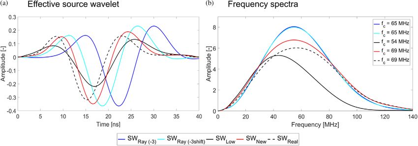
Improving crosshole ground-penetrating radar full-waveform inversion results 9

Figure 5 RMS misfit curves of the different FWI approaches of the synthetic case study I. Blue graph represents the RMS of the standard FWI
using the ray-based starting models (iteration numbers are shown at the top with a red label). The cyan graph represents the RMS behaviour
for the PBED inversion scheme based on Meles et al. (2012). Black and red graphs represent the new PEBDD inversion scheme using the first
updated and second updated source wavelets, respectively. The green graph shows the new FWI RMS according to the updated starting models
including εr and σ (Appendix) by using PEBDD inversion scheme. Note that on the left side of the dashed lines, the progressive expansion of
the bandwidths of effective source wavelets and observed data was used, while on the right side the FWI was performed considering the full
bandwidth of all data. New PEBDD inversion RMS values are increased before 70 iterations (red and black lines), because of the larger amplitude
values of the source wavelet and the observed data.

exemplary data set (Fig. 6c), we find most of the regions in              ing models ModelNew for the following FWI results and the
the tomograms a small misfit is visible, but for some domains             updated source wavelet. Following the flowchart (Fig. 1b, red
a increased difference can still be noticed. Considering that the         box), the effective source wavelet SWLow is updated using the
real effective source wavelet has a centre frequency of 69 MHz            new starting models ModelNew and the wavelet SWRay . The ef-
and the stochastic model has an approximate average permit-               fective source wavelet SWLow together with the starting mod-
tivity value of 18, the corresponding wavelength of the GPR               els ModelNew is used to calculate the FWI as shown in Fig. 4
signal is 1.03 m. Comparing the model cell size of 0.09 m with            (a and b) (second column) using the full data set. By compar-
the wavelength 1.03 m, it is hard to match all the features of            ing the RMS curve behaviour of this inversion (black graph
the stochastic model especially when the contrast is relatively           in Fig. 5; black graph is covered by red graph before 71 itera-
high.                                                                     tions), we can notice that first the RMS is stepwise increased
      Following our new introduced approach of the progres-               until the full data are used and the RMS curve with the full
sively expanded bandwidths of the modelled and observed                   data are decreased after 23 iterations to a final value of 6.9749
data (PEBDD), we applied the different bandpass filters as                × 10−7 . The misfits between the input and resolved tomo-
shown in Fig. 1(a) to the standard effective source wavelet               grams (Fig. 4d and e) and the data misfit (Fig. 6c) are slightly
SWRay (different effective source wavelets shown in Fig. 2)               better than using the standard FWI approach.
and the observed data. For this study, we choose the op-                        These updated FWI results are in the last step considered
timal five iterations for the sub-data FWI by comparing                   to update the effective source wavelet a last time (SWNew in
with other iterations values. The first sub-data FWI started              Fig. 3a and b, red source wavelet) by using the new FWI
from the filtered sub-source wavelet and filtered sub-observed            εr results with SWLow in the deconvolution approach. The cor-
data with bandwidth 12–16 MHz and the ray-based start-                    responding final FWI results (Fig. 4, third column) are derived
ing models ModelRay . Every five iterations the bandpass is in-           with the SWNew and ModelNew as the starting models. Note
creased by 4 MHz until the final cut-off frequency of 68 MHz              that we also tested the new approach with the both permit-
is reached. The final permittivity FWI results using the max-             tivity and conductivity starting models based on the maxi-
imum bandwidth sub-data are shown in Fig. 4a (title is ‘Up-               mum bandwidth sub-data (Fig. A.1a). The obtained FWI re-
dated – εr ’). Combining the conductivity starting model with             sults (Fig. A.1b) indicate the results with SWNew ( εr + σ ) did
a homogeneous value of 13 mS/m, we construct the new start-               not improve significantly than the FWI results with the SWNew

© 2021 The Authors. Near Surface Geophysics published by John Wiley & Sons Ltd on behalf of European Association of
Geoscientists and Engineers., Near Surface Geophysics, 1–23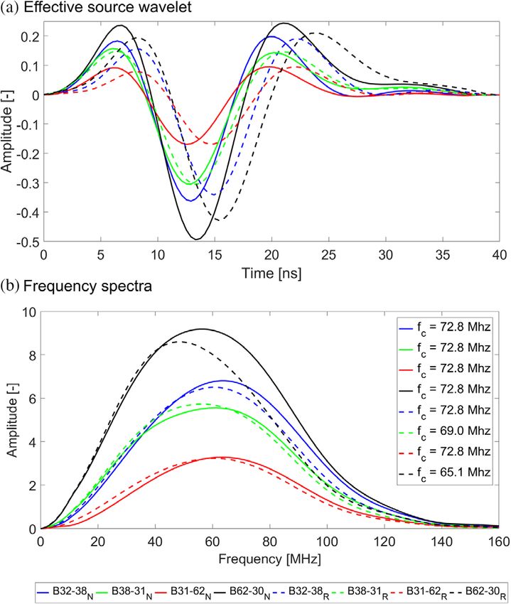
10 Z. Zhou, A. Klotzsche and H. Vereecken

Figure 6 (a) Observed data, (b) modelled data based on the FWI results and (c) differences between the observed and modelled data for one
exemplary data set of transmitter location at 5.69 m depth (see input models and black arrow for the transmitter location in Fig. 4). Note the
amplitudes in (a–c) are normalized to the maxima amplitude of the real observed data (shown range from −7 × 10⁻¹ to 7 × 10⁻¹ ). The mean
absolute errors of the permittivity and conductivity between the real input and the different FWI results are shown along (d) the horizontal
cross-section and (e) vertical direction.

                   © 2021 The Authors. Near Surface Geophysics published by John Wiley & Sons Ltd on behalf of European Association of
                                                                            Geoscientists and Engineers., Near Surface Geophysics, 1–23
Improving crosshole ground-penetrating radar full-waveform inversion results 11
and ModelNew as the starting models; therefore, we consider Table 1 Comparison of the different FWI approaches for synthetic
in further applications only the permittivity updated start- case study I using the mean absolute error between the real input
models and the different FWI results for the entire 2D domain, and
ing model. For comparisons, we performed the approach of
the root-mean-squared RMS error between observed and modelled
Meles et al. (2012) that only uses the sub-source wavelets in radar traces represents residual values. Percentages in parentheses in-
the FWI, which means using the progressively bandwidth ex- dicate the ratio of the single FWI RMS to the standard FWI RMS
panded modelled data (PBED), while the observed data in- with SWRay , while a decreased value means the higher improvement
clude the full bandwidth (Fig. 4, fourth column). Note that efficiency
the generated FWI results (including εr and σ ) with the maxi- Real models MAE (εr ) MAE (σ ) RMS (10−7 )
mum bandwidth sub-source wavelet are the new starting mod-
els (only show the εr starting model with the title M − εr in FWI (SWRay ) 2.0056 2.2043 6.9945 (100%)
Fig. 4a) for the following FWI with full bandwidth data. FWI (SWLow ) 1.9338 2.2718 6.9749 (99.7%)
FWI (SWNew ) 1.7309 2.0351 2.8996 (41.5%)
The FWI results using the SWNew show the smallest mis-
FWI (SWRay + M) 2.5560 2.5430 8.6499 (123.7%)
fit of the resolved tomograms and the smallest final RMS,
FWI (SWNew ( εr + σ )) 1.8500 2.1851 3.8620 (55.2%)
indicating that this approach is able to resolve the input to-
mograms best. Note that we are able to improve the FWI re-
sults for the permittivity and the conductivity by 13.7% and (2012) are unrealistic. By computing the absolute errors be-
7.7% in comparison to the standard FWI models using SWRay tween these different FWI results and the real input models
by comparing the MAE values of the two approaches, re- in 2D domain (Fig. 4d and e), we can find that the second-
spectively (Table 1). Especially, the small-scale structures close updated FWI results with SWNew are close to the input mod-
to the boreholes are clearer and more accurately resolved as els indicated by the smallest MAE values (Table 1). By inves-
by the standard method. By comparing the final RMS curves tigating the fit between the observed and the FWI modelled
(only show the max iterations until 101 or 31; the same for GPR data, generally a good fit can be observed for all the FWI
Fig. 9) of the five different FWI results (green graph based on results (one example shown for transmitter depth 5.69 m in
results shown in the Appendix), the second-updated FWI re- Fig. 6a and b), but analysing the differences (Fig. 6c) in more
sults with the wavelet SWNew indicate the best convergence detail, we notice that the FWI using SWNew shows the smallest
behaviour resulting in the smallest residual value of 2.8996 misfit.
× 10−7 after 50 iterations (red curve in Fig. 5). Comparisons In order to describe the regional differences of differ-
of four different FWI εr and σ results in 2D domain (Fig. 4b ent FWI models, we computed the MAE between the in-
and c) show the FWI results with the approach of Meles et al. put stochastic models and the FWI model results along the
Figure 7 (a) Comparisons of the different effective source wavelets used for synthetic case study II. The source wavelet used to generate the
‘observed data’ is indicated with a dashed black graph. (b) Frequency spectra comparisons from 0 to 140 MHz for the five different effective
source wavelets. The legend values in (b) indicate these effective centre frequencies for different steps.
© 2021 The Authors. Near Surface Geophysics published by John Wiley & Sons Ltd on behalf of European Association of
Geoscientists and Engineers., Near Surface Geophysics, 1–2312 Z. Zhou, A. Klotzsche and H. Vereecken
Figure 8 Overview of the FWI results using different approaches. Left, real input models based on the stochastic models. (a) Permittivity starting
models and corresponding FWI results for (b) εr and (c) σ for the different FWI approaches. The applied effective source wavelets are named
in titles of the Fig. 8. Image plots of the absolute error between the input models and final FWI results for (d) εr and (e) σ for the different
approaches. The mean absolute errors of the entire 2D domain are shown in parentheses.
© 2021 The Authors. Near Surface Geophysics published by John Wiley & Sons Ltd on behalf of European Association of
Geoscientists and Engineers., Near Surface Geophysics, 1–23Improving crosshole ground-penetrating radar full-waveform inversion results 13
Figure 9 RMS misfit curves of the different FWIs for synthetic case study II. The blue and cyan graphs represent the FWI RMS convergence
behaviours using the source wavelets SWRay (−3) and SWRay (−3 shift) based on enforcing a smaller εr starting model (iterations are from 1 to 31 at
red label on the top), respectively. Black and red graphs represent the new PEBDD inversion scheme using the first updated and second updated
effective source wavelets, respectively. Note that before the dashed lines, the progressively expanded of the bandwidths of source wavelets and
observed data are used, while on the right side the FWI with the full bandwidth of all data are performed.
Table 2 Comparison of the different FWI approaches of the mean results with a smaller MAE in the vertical direction between
absolute error between the real input models and the different FWI 4.0 m and 5.5 m depth in comparison to other depths, where
models for the entire 2D domain for synthetic case study II. RMS rep-
the small-scale structures are located. A small increase of the
resents residual values between observed and modelled radar traces.
Percentages in parentheses indicate the ratio of the other FWI RMS
MAE at 5.5 m depth can be noticed at the lower boundary of
to the standard FWI RMS with SWRay (−3) , the lower value means the the small-scale high permittivity zone. For both horizontal and
higher improvement efficiency vertical directions, the FWI results based on the SWNew show
the lowest MAE, in contrast to the other FWI results. Com-
Real models MAE (εr ) MAE (σ ) RMS (10−7 )
paring the FWI results and the related MAE, we can conclude
FWI (SWRay (−3) ) 3.6152 2.3394 9.1843 (100%) that our newly updated PEBDD scheme is effective to enhance
FWI (SWRay (−3shift) ) 2.4839 2.2683 8.3326 (90.7%) the complicated synthetic models’ FWI results for permittivity
FWI (SWLow ) 2.1968 3.1050 18.366 (200.0%) and conductivity, in contrast to the standard FWI approach.
FWI (SWNew ) 2.1027 2.0498 3.6288 (39.5%)
Synthetic case study II: Permittivity starting model beyond the
horizontal direction (Fig. 6d) and the vertical direction
half-wavelength criteria
(Fig. 6e) for εr and σ , respectively. The smallest MAE of the
horizontal direction can be observed in the central part of the In the presence of high contrast layers, ray-based results are
tomograms between 3.0 m and 5.0 m (Fig. 6d). For all re- often erroneous and need to be updated to fulfill the half-
sults, the MAE of the horizontal direction increases towards wavelength starting model criteria for the standard FWI. Here,
the boundaries of the inversions domain, meaning the bore- we want to demonstrate the potential of the PEBDD scheme,
holes of the cross-section (Fig. 6d). The MAE in the horizon- which also allows starting models that are beyond the half-
tal direction and an increase in MAE towards the boreholes wavelength criteria. Therefore, we perform a second synthetic
are related to the acquisition geometry and the related dis- case study with the same stochastic input models as before
tribution of the ray coverage between the boreholes. Ober- and enforce the permittivity starting model to provide mod-
röhrmann et al. (2013) showed already that the resolution is elled data more than half a wavelength away from the mea-
highly affected by the acquisition geometry and depends on sured data by using a smaller εr model. The changed εr start-
the ray coverage. The MAE along the vertical direction shows ing model was obtained by subtracting three from the nor-
more fluctuations around 2, while the results in horizontal di- mal ray-based εr model in the entire domain (Fig. 8a, title is
rection are smoother. Interestingly, all the FWI results (except ‘Ray –εr (−3)’). The conductivity starting model is unchanged
the approach based on Meles et al., 2012) show improved with a homogeneous value of 13 mS/m. We follow the same
© 2021 The Authors. Near Surface Geophysics published by John Wiley & Sons Ltd on behalf of European Association of
Geoscientists and Engineers., Near Surface Geophysics, 1–2314 Z. Zhou, A. Klotzsche and H. Vereecken
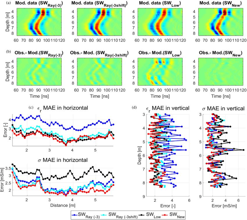
Figure 10 (a) Modelled data based on the FWI results and (b) differences between the observed and modelled data for the transmitter at 5.69 m
depth (see input models and black arrow for the transmitter location in Fig. 8). Note the amplitudes in (a) and (b) are normalized to the maxima
amplitude of the real observed data (shown range from −7 × 10⁻¹ to 7 × 10⁻¹ ). The mean absolute errors of the permittivity and conductivity
between the input models and the different FWI results are shown along (c) horizontal cross-section and (d) vertical direction.
approach as in the synthetic study case I and obtained the dif- sating for this by starting later in time (blue curves in Fig. 7a
ferent updated effective source wavelets (Fig. 7) and FWI re- and b). Note that a good effective source wavelet needs to
sults (Fig. 8). start at 0 ns (Klotzsche et al., 2019b). The FWI results (first
First, we estimate the effective source wavelet SWRay (−3) column in Fig. 8b and c) based on these starting models and
based on the erroneous starting models ModelRay−3 . We can the effective source wavelet SWRay (−3) fulfil the stopping crite-
clearly notice that the SWRay (−3) based on the erroneous start- ria after 24 iterations and no remaining gradients are present.
ing models is shifted in time to the right (Fig. 7a). This is indi- The FWI RMS curve by using the source wavelet SWRay (−3)
cating that the permittivity starting model is currently too far is shown with the blue curve in Fig. 9. Generally, the re-
away from the input models and that the wavelet is compen- sulting FWI results show a lower εr than the input model,
© 2021 The Authors. Near Surface Geophysics published by John Wiley & Sons Ltd on behalf of European Association of
Geoscientists and Engineers., Near Surface Geophysics, 1–23Improving crosshole ground-penetrating radar full-waveform inversion results 15
Figure 11 (a) Ray-based εr results and (b) FWI εr results using the
selected maximum frequency bandwidth sub-data. Note that results
shown in (b) are used as starting models for the full bandwidth in-
version of the experimental Krauthausen data. And a homogeneous Figure 12 (a) Comparisons of the effective source wavelets estimated
conductivity starting model of 13 mS/m was used for all inversions. based on ray-based models (dashed graphs) and the updated source
wavelets of the PEBBD scheme (solid graphs) for the four cross-
sections in time domain for the experimental data of the Krauthausen
demonstrating that the εr result gets trapped in a local min- test site. (b) Corresponding frequency spectra of standard and updated
imum of the inversion process (Fig. 8b, first column). This is effective source wavelets. The legend values in (b) indicate these effec-
tive centre frequencies for different cross-sections.
also indicated by the differences between the input model and
FWI results in Fig. 8(d), where many regions are present that
show differences with more than three in permittivity. Note approach. For the first sub-data FWI, the first starting
that this inversion still fulfils most of the criteria for a good models ModelRay−3 are used. The final FWI εr results using
inversion process. The only indicators that the inversion is too the maximum bandwidth sub-data (Fig. 8a, updated – εr (−3))
far away from the input model are provided by the effective and the homogeneous σ model with 13 mS/m are used as the
source wavelet that is shifted in time and the high MAE (not new updated starting models ModelNew−3 . It can be noticed
available for experimental data applications). To fulfil the cri- that the updated permittivity starting model shows generally
teria that the effective source wavelet needs to start at 0 ns, higher values in the entire domain and the model is much
we shifted in the next step the source wavelet by −4 ns in the closer to the ray-based model used in the synthetic study I,
time domain SWRay (−3shift) (cyan curves in Fig. 7a and b) to indicating that the PEBDD approach is able to enhance the
ensure that it starts at 0 ns. The corresponding FWI results erroneous starting model (compare Figs 4a and 8a). The up-
(Fig. 8b and c, second column) show a better reconstruction dated starting models are considered to derive SWLow before
of the permittivity results than the previous inversion, and the performing the FWI.
final RMS value after 30 iterations is 8.3326 × 10⁻⁷ (cyan The updated FWI results using SWLow show improved
curve in Fig. 9). Meanwhile the FWI σ results are better than permittivity results and more continuous structures, although
the FWI σ results with SWRay (−3) (Fig. 8c, columns first and the conductivity performs less good indicated by the image
second). differences (Fig. 8b and c, third column) and the higher RMS
Similar to the previous synthetic case І, we apply the value for the final iteration (Fig. 9, black graph). The final per-
same bandpass filters for the same number of iterations mittivity results of this inversion and SWLow are used to update
to the shifted effective source wavelet SWRay (−3shift) to en- the effective wavelet a last time to SWNew (Fig. 7a and b, red
hance the reconstruction of the FWI results with the PEBDD source wavelet). The corresponding FWI results (Fig. 8b and c,
© 2021 The Authors. Near Surface Geophysics published by John Wiley & Sons Ltd on behalf of European Association of
Geoscientists and Engineers., Near Surface Geophysics, 1–2316 Z. Zhou, A. Klotzsche and H. Vereecken
Figure 13 Standard FWI results of (a) εr and (c)
σ of the four cross-sections. Updated FWI results
of (b) εr and (d) σ based on the new εr starting
models (Fig. 11b) and corresponding updated new
effective source wavelets (solid graphs in Fig. 12).
Dashed lines mark the CPT data locations between
the boreholes.
fourth column) after 50 iterations are derived with the SWNew The MAE values (shown in titles of Fig. 8d and e) and
and ModelNew−3 as the starting models. These results show an behaviour of the RMS curves (Fig. 9) are best for the second-
improved reconstruction of the permittivity and the conduc- updated FWI results with the wavelet SWNew and indicate the
tivity results in comparison to the previous FWI results. Fur- best FWI results (more details in Table 2). Analysing the mis-
thermore, comparisons of the absolute error tomograms for fit between the observed and FWI modelled data shows that
different FWI εr and σ results in 2D domain (Fig. 8d and e) the second-updated FWI results provide the best fit and in-
show that the second-updated FWI results with the wavelet dicates that this inversion obtained a model that describe the
SWNew are the most accurate reconstruction of the input data well and best, while for the other three FWI results a
models. significant misfit can be observed (Fig. 10a and b, exemplary
© 2021 The Authors. Near Surface Geophysics published by John Wiley & Sons Ltd on behalf of European Association of
Geoscientists and Engineers., Near Surface Geophysics, 1–23Improving crosshole ground-penetrating radar full-waveform inversion results 17
Table 3 Comparison of the different FWI approaches for the experimental data set of the Krauthausen test site. RMS represents residual values
between observed and modelled radar traces. Percentages in parentheses indicate the ratio of the new FWI RMS to the standard FWI RMS
with SWRay , the lower value means the higher improvement efficiency. Correlation coefficient R and RMS between 1D εr FWI and the CPT
data (CPT porosity has been converted into εr ) represent the reliability of the FWI results, the larger R and the lower RMS values mean the FWI
results are closer to the real values
Borehole No. (distance between boreholes) 32–38 (5.13 m) 38–31 (4.99 m) 31–62 (3.83 m) 62–30 (6.16 m)
Standard FWI RMS (10−7 ) (SWRay ) 8.5055 9.4156 9.1763 7.0538
New FWI RMS (10−7 ) (SWNew ) 6.8210 7.1789 7.8503 5.4136
(80.2%) (76.2%) (85.5%) (76.7%)
R (Sta-FWI:CPT) 0.8105 0.9032 0.8301 0.8830
R (New FWI:CPT) 0.8409 0.8973 0.8408 0.8723
RMS (Sta-FWI:CPT) 2.6807 1.9307 2.5131 2.1026
RMS (New FWI:CPT) 1.9054 2.1503 1.5224 1.7333
Figure 14 Permittivity comparisons derived from cone penetration test (CPT) data (black), standard FWI εr results (blue) and the updated new
FWI εr results (red) along CPT profiles between boreholes (see Fig. 13 for locations).
for transmitter at 5.69 m depth). To describe the regional els for experimental GPR data can be reduced and the appli-
differences of different FWI models, we compute the MAE cation to field data could be much easier.
between the stochastic input models and the FWI model re-
sults along the horizontal direction (Fig. 10c) and the verti-
Experimental ground-penetrating radar data studies
cal direction (Fig. 10d) for εr and σ , respectively. Thereby, we
can notice that the FWI εr results with SWRay (−3) display the As a final test, we applied the new PEBDD approach to
largest MAE values for both directions. The FWI σ results an experimental data set from the Krauthausen test site in
with SWLow (black curves) have a large MAE, which implies Germany. The Krauthausen study site is located approxi-
that they cannot be resolved by only using the first-updated mately 10 km northwest of the city Düren in Germany and
effective source wavelet in time when the starting models are a detailed description of the site can be found in Vereecken
too far away from the real models. Finally, we can conclude et al. (2000). In the last decades, many hydrological and geo-
that the progressively expanded bandwidth scheme can not physical field techniques have been applied on this site to
only improve the FWI results, but also that it is able to re- study the aquifer spatial distribution and flow characteris-
trieve accurate FWI results for starting models more than a tics, including flowmeter tests (Li et al., 2008), tracer experi-
half-wavelength away from the measured data. Therefore, a ments (Vereecken et al., 2000; Vanderborght and Vereecken,
lot of previous detailed work to construct good starting mod- 2001), cone penetration tests (Tillmann et al., 2008) and GPR
© 2021 The Authors. Near Surface Geophysics published by John Wiley & Sons Ltd on behalf of European Association of
Geoscientists and Engineers., Near Surface Geophysics, 1–23You can also read