RA3 is a reference-guided approach for epigenetic characterization of single cells
←
→
Page content transcription
If your browser does not render page correctly, please read the page content below
ARTICLE
                  https://doi.org/10.1038/s41467-021-22495-4                 OPEN

                  RA3 is a reference-guided approach for epigenetic
                  characterization of single cells
                  Shengquan Chen             1,2,4,   Guanao Yan3,4, Wenyu Zhang2, Jinzhao Li2, Rui Jiang1 ✉ & Zhixiang Lin                              2✉

                  The recent advancements in single-cell technologies, including single-cell chromatin acces-
                  sibility sequencing (scCAS), have enabled profiling the epigenetic landscapes for thousands
1234567890():,;

                  of individual cells. However, the characteristics of scCAS data, including high dimensionality,
                  high degree of sparsity and high technical variation, make the computational analysis chal-
                  lenging. Reference-guided approaches, which utilize the information in existing datasets, may
                  facilitate the analysis of scCAS data. Here, we present RA3 (Reference-guided Approach for
                  the Analysis of single-cell chromatin Accessibility data), which utilizes the information in
                  massive existing bulk chromatin accessibility and annotated scCAS data. RA3 simultaneously
                  models (1) the shared biological variation among scCAS data and the reference data, and (2)
                  the unique biological variation in scCAS data that identifies distinct subpopulations. We show
                  that RA3 achieves superior performance when used on several scCAS datasets, and on
                  references constructed using various approaches. Altogether, these analyses demonstrate
                  the wide applicability of RA3 in analyzing scCAS data.

                  1 Ministryof Education Key Laboratory of Bioinformatics, Bioinformatics Division at the Beijing National Research Center for Information Science and
                  Technology, Center for Synthetic and Systems Biology, Department of Automation, Tsinghua University, Beijing, China. 2 Department of Statistics, The
                  Chinese University of Hong Kong, Hong Kong SAR, China. 3 School of Mathematical Sciences, Zhejiang University, Hangzhou, China. 4These authors
                  contributed equally: Shengquan Chen, Guanao Yan. ✉email: ruijiang@tsinghua.edu.cn; zhixianglin@cuhk.edu.hk

                  NATURE COMMUNICATIONS | (2021)12:2177 | https://doi.org/10.1038/s41467-021-22495-4 | www.nature.com/naturecommunications                               1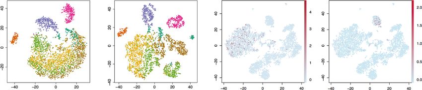
ARTICLE                                                                 NATURE COMMUNICATIONS | https://doi.org/10.1038/s41467-021-22495-4

C
        hromatin accessibility is a measure of the physical access           data, RA3 effectively extracts biological variation in single-cell
        of nuclear macromolecules to DNA and is essential for                data for downstream analyses, such as data visualization and
        understanding the regulatory mechanism1,2. For rapid and             clustering. RA3 not only captures the shared biological variation
sensitive probing of chromatin accessibility, assay for                      between single-cell chromatin accessibility data and reference
transposase-accessible chromatin using sequencing (ATAC-seq)                 data, but also captures the unique biological variation in single-
directly inserts sequencing adaptors into accessible chromatin               cell data that is not represented in the reference data. RA3 can
regions using hyperactive Tn5 transposase in vitro3. With the                model known covariates, such as donor labels. Through com-
recent advancements in technology, single-cell chromatin acces-              prehensive experiments, we show that RA3 consistently outper-
sibility sequencing (scCAS) further enables the investigation of             forms existing methods on datasets generated from different
epigenomic landscape in individual cells4,5. However, the analysis           platforms, and of diverse sample sizes and dimensions. In addi-
of scCAS data is challenging because of its high dimensionality              tion, RA3 facilitates trajectory inference and motif enrichment
and high degree of sparsity, as the low copy number (two of a                analysis for more biological insight on the cell subpopulations.
diploid-genome) of DNA leads to only 1–10% capture rate for the
hundreds of thousands of possible accessible peaks6. The
                                                                             Results
proposed approaches for the analysis of single-cell RNA-seq
                                                                             The RA3 model. RA3 is a generative model based on the fra-
(scRNA-Seq) data thus present limitations due to the novelty and
                                                                             mework of probabilistic PCA33, and it decomposes the total
assay-specific challenges of extreme sparsity and tens of times
                                                                             variation in scCAS data into three components: the component
higher dimensions6.
                                                                             that captures the shared biological variation with reference data,
   Several computational algorithms have been proposed to
                                                                             the component that captures the unique biological variation in
analyze scCAS data. chromVAR assesses the variation of chro-
                                                                             single cells, and the component that captures other variations
matin accessibility using groups of peaks that share the same
                                                                             (Fig. 1a). More specifically, the first component utilizes the prior
functional annotations7. scABC calculates weights of cells based
                                                                             information of the projection vectors learned from reference data,
on the number of distinct reads within the peak background and
                                                                             and it captures the variation in single-cell data that is shared with
then uses weighted k-medoids to cluster the cells8. cisTopic
                                                                             the reference data. Choice of the reference data is flexible: it can
applies latent Dirichlet allocation model to explore cis-regulatory
                                                                             be the chromatin accessibility profiles of bulk samples or pseudo-
regions and characterizes cell heterogeneity from the generated
                                                                             bulk samples by aggregating single cells. In practice, the reference
regions-by-topics and topics-by-cells probability matrices9.
                                                                             data can be incomplete: novel cell types or novel directions of
Cusanovich et al. proposed a method that performs the term
                                                                             biological variation that are not captured in the reference data can
frequency-inverse document frequency transformation (TF-IDF)
                                                                             be present in the single-cell data. The second component captures
and singular value decomposition iteratively to get the final fea-
                                                                             the unique biological variation in single-cell data that is not
ture matrix5,10. Scasat uses Jaccard distance to evaluate the dis-
                                                                             present in the reference data: it incorporates the spike-and-slab
similarity of cells and performs multidimensional scaling to
                                                                             prior to capture the direction of variation that separates a small
generate the final feature matrix11. SnapATAC segments the
                                                                             subset of cells from the other cells, since there may be rare cell
genome into fixed-size bins to build a bins-by-cells binary count
                                                                             types that are not captured in the reference data. The spike-and-
matrix and uses principal component analysis (PCA) based on
                                                                             slab prior also facilitates RA3 to distinguish biological variation
the Jaccard index similarity matrix to obtain the final feature
                                                                             from technical variation, assuming that the direction of variation
matrix12. SCALE combines a variational autoencoder and a
                                                                             that separates a small subset of cells more likely represents bio-
Gaussian mixture model to learn latent features of scCAS data13.
                                                                             logical variation. The third component captures the other varia-
Destin is based on weighted PCA, where the peaks have different
                                                                             tions in single-cell data, and it likely represents the technical
weights based on the distances to transcription start sites and the
                                                                             variation. Other than the three components, RA3 includes
relative frequency of the peaks in ENCODE data14–16.
                                                                             another term to model known covariates. The first and second
   Incorporating reference data in analyzing single-cell genomic
                                                                             components are used for downstream analyses, and we present
data can better tackle the high level of noise and technical var-
                                                                             results on data visualization, cell clustering, trajectory inference
iation in single-cell genomic data. Most reference-guided meth-
                                                                             and motif enrichment analysis.
ods are designed for single-cell transcriptome data, and they focus
primarily on cell type annotation using reference data and marker
genes, which limits their application to other downstream ana-               RA3 decomposes variation in single-cell data. We first use a
lyses, such as data visualization and trajectory inference17–27. For         simple example as a proof of concept to demonstrate RA3. We
the analysis of single-cell chromatin accessibility data, SCATE28            collected human hematopoietic cells with donor label BM0828
was recently proposed to reconstruct and recover the “true”                  from a bone marrow scATAC-seq dataset29 (referred as the
chromatin accessibility level for each region in scCAS data uti-             human bone marrow dataset). To reduce the noise level, we first
lizing the information in bulk chromatin accessibility data, which           adopted a feature selection strategy similar to scABC and SCALE
is similar to the goal of imputation methods developed for                   (Methods). We performed the TF-IDF transformation to nor-
scRNA-Seq data. Massive amounts of bulk chromatin accessibility              malize the scATAC-seq data matrix, implemented PCA, and then
data have been generated from diverse tissues and cell lines15,16.           performed t-distributed stochastic neighbor embedding (t-SNE)34
The amount of scCAS data is rapidly increasing4,5,10,29,30.                  to reduce the dimension to two for visualization. This approach
Meanwhile, computational tools that collect chromatin accessi-               (TF-IDF + PCA) is similar to that in Cusanovich20185,10, which
bility data and efficiently compute chromatin accessibility over              is among the top three methods suggested in a recent benchmark
the genomic regions facilitate the construction of reference                 study6. More discussions on TF-IDF transformation are provided
data31,32.                                                                   in the Methods section. It is hard to separate the majority of the
   To utilize the information in existing chromatin accessibility            cell types using TF-IDF + PCA, and only CLP and MEP cells are
datasets for the analysis of scCAS data, we propose a probabilistic          moderately separated from the other cells (Fig. 1b). We then
generative model, RA3, in short for Reference-guided Approach                collected a reference data: bulk ATAC-seq samples from four
for the Analysis of single-cell chromatin Acessibility data.                 parent nodes in the hematopoietic differentiation tree29, includ-
Incorporating reference data built from bulk ATAC-seq data,                  ing samples that correspond to HSC, MPP, LMPP, and CMP cells
bulk DNase-seq data, and pseudo-bulk data by aggregating scCAS               after fluorescent activated cell sorting. The genomic regions in the

2                NATURE COMMUNICATIONS | (2021)12:2177 | https://doi.org/10.1038/s41467-021-22495-4 | www.nature.com/naturecommunications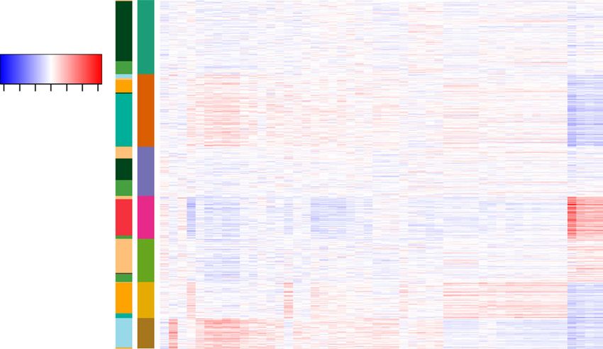
NATURE COMMUNICATIONS | https://doi.org/10.1038/s41467-021-22495-4                                                                         ARTICLE

Fig. 1 The reference-guided approach for the analysis of scCAS data. a A graphical illustration of the RA3 model. RA3 decomposes the variation in scCAS
data into three components: the component that captures the shared biological variation with reference data, the component that captures the unique
biological variation in single-cell data, and the component that captures other variations. b t-SNE visualization of the cells from donor BM0828 using latent
features obtained from TF-IDF + PCA. c t-SNE visualization of the cells from donor BM0828 using latent features obtained from bulk projection. d We
calculated the residuals after the bulk projection. PCA was performed on the residuals, followed by t-SNE visualization. e The learned second component
with the spike-and-slab prior in RA3. f t-SNE visualization using the first two components learned by RA3. TF-IDF term frequency-inverse document
frequency transformation, PCA principal component analysis.

reference data are matched with that in the single-cell data. We                method was not as good as our simple approach (Supplementary
first considered a simple approach, referred as the bulk projection              Fig. 1a).
approach, to utilize the information in the reference data: (1) we                 The bulk projection approach implicitly assumes that all the
applied PCA on bulk ATAC-seq data; (2) we used the projection                   biological variation is shared in single-cell and the reference data,
vectors learned from bulk data to project single-cell data after TF-            as it only uses the projection vectors learned from the reference
IDF normalization; (3) for visualization, we applied t-SNE on the               data and do not use single-cell data to learn the projection
projected data to further reduce the dimension to two. This                     vectors. In this example, using the projection vectors from
simple approach significantly improves the separation of the cell                reference data alone cannot distinguish CLP from the other cells,
types (Fig. 1c). A method similar to the above approach was                     since the variation of CLP cells is not captured in the reference
proposed in Buenrostro et al.29, but the performance of the                     data. We took residual after the bulk projection, and implemented

NATURE COMMUNICATIONS | (2021)12:2177 | https://doi.org/10.1038/s41467-021-22495-4 | www.nature.com/naturecommunications                                   3
ARTICLE                                                                 NATURE COMMUNICATIONS | https://doi.org/10.1038/s41467-021-22495-4

PCA + t-SNE on the residual matrix: most cells other than MEP                diverse biological context collected from ENCODE, which can be
and CLP cells are mixed together, which indicates the presence of            used as the reference data. Note that this approach requires the
strong technical variation in the residual matrix (Fig. 1d). This            BAM files for the reference samples to calculate accessibility, an
observation suggests that including the direction of variation               alternative approach that does not require BAM files will be
learned from single-cell data may help to separate CLP cells, but            discussed later. With the peak information in the human bone
the direction needs to be carefully chosen because of the strong             marrow dataset29, we used OPENANNO to construct the refer-
technical variation. A schematic plot for the desired direction of           ence data with samples of diverse biological context. The refer-
variation to learn from single-cell data is shown in Fig. 1d: it             ence data constructed in this way achieved similar performance as
separates a small subset of cells from the other cells, and the              the manually curated reference data using only the relevant cell
technical variation is weaker along that direction.                          types (Supplementary Fig. 1b).
   Our proposed RA3 models the data after TF-IDF transforma-                    We next applied RA3 to three other single-cell datasets: (1) a
tion. To overcome the limitation of the bulk projection approach,            mixture of human GM12878 and HEK293T cells (referred as the
RA3 not only incorporates prior information from the projection              GM/HEK dataset)5; (2) a mixture of human GM12878 and HL-60
vectors learned from the reference data as the first component in             cells (referred as the GM/HL dataset)5; (3) an in silico mixture of
the decomposition of variation, but also incorporates a second               H1, K562, GM12878, TF-1, HL-60 and BJ cells (referred as the
component to model the unique biological variation in single-cell            InSilico mixture dataset)4. We first manually constructed the
data. The key for the second component in RA3 is a spike-and-                reference using BAM files of bulk DNase-seq samples from
slab prior35,36, which facilitates the model to detect directions that       the relevant cell lines (Methods). The performance significantly
lead to good separation of a small number of cells from the other            improved over the approach not using reference data (Fig. 2a,b
cells, and not necessarily directions with the largest variation.            and Supplementary Fig. 1d, e), which indicates that the abundant
Using the direction of the largest variation can be problematic              BAM files of bulk chromatin accessibility profiles in the literature
given that the technical variation can be strong. Applying RA3 to            can be fully used to help the analysis of scCAS data. When we
the example, the second component with the spike-and-slab prior              constructed the reference data with OPENANNO using all the
successfully distinguishes CLP cells (Fig. 1e). We note that the             871 bulk samples (Methods), the performance of RA3 is
labels for CLP cells are not used in RA3 to detect the direction             comparable with the implementation using only the relevant cell
that separates CLP cells. In this example, RA3 effectively utilizes          lines for reference (Fig. 2c and Supplementary Fig. 1d, e).
the prior information in reference data to separate CMP, GMP,                   We also considered an alternative approach to construct the
HSC/MPP, LMPP, and MEP cells, and it also captured the unique                reference using only the peak files (BED files) of the reference
variation in single-cell data, which separates CLP cells from GMP            samples, to address the situation when BAM files are not
and LMPP cells (Fig. 1f). The loadings of the second component               available. The reference data can be constructed by counting the
in RA3 provide functional insight on the cell subpopulations.                number of peaks in reference sample that overlap with every peak
Using the top 1000 peaks with largest magnitude in the loadings              in single-cell data (Methods). This approach to construct the
of the second component (we focus on peaks with negative                     reference data also led to satisfactory performance (Fig. 2d and
loadings as the sign of H2 for the identified cell subpopulation is           Supplementary Fig. 1c–e), which suggests that we can build useful
mostly negative), we performed Genomic Region Enrichment of                  reference with the peak files of bulk data when BAM files are not
Annotation Tool (GREAT)37 analysis to identify significant                    available. Therefore, databases that collect more comprehensive
pathways associated with the identified cell subpopulation in                 biological samples but only provide the peak information for each
the second component (Methods). The top five pathways with                    bulk sample, such as Cistrome DB32, may further facilitate the
smallest p values from the binomial test are regulation of                   usage of RA3.
lymphocyte activation, Fc receptor signaling pathway, immune
response-regulating cell surface receptor signaling pathway,
immune response-activating cell surface receptor signaling path-             RA3 incorporates pseudo-bulk data as reference. It can be
way, and positive regulation of lymphocyte activation (see                   difficult to obtain the bulk samples for certain cell populations,
Supplementary Table 1 for the complete enrichment results).                  especially for the cells in frozen or fixed tissues, where cell sorting
These enriched pathways are consistent with the function of CLP              is challenging to implement. The recent efforts of cell atlas con-
cells: CLP cells serve as the earliest lymphoid progenitor cells and         sortiums have generated massive amounts of single-cell tran-
give rise to T-lineage cells, B-lineage cells, and natural killer (NK)       scriptome data for whole organisms38–47, and single-cell
cells. To summarize, the second component in RA3 not only                    chromatin accessibility data are rapidly increasing4,5,10,29,30. We
identifies the rare cell subpopulation, but also provides functional          can construct pseudo-bulk reference data by aggregrating single
insight of the identified cell subpopulation.                                 cells of the same type/cluster to alleviate the high degree of
                                                                             sparsity in scCAS data. As a proof of concept, we first look at a
                                                                             single-nucleus ATAC-seq dataset generated from mouse fore-
RA3 builds effective reference from massive bulk data. The                   brain (referred as the mouse forebrain dataset)30, where the cell
previous example of hematopoietic cells utilizes reference data              type labels were provided, including astrocyte (AC), three sub-
constructed from manually curated bulk samples that have rele-               types of excitatory neuron (EX1, EX2, and EX3), two subtypes of
vant biological context with the single-cell data. The cellular              inhibitory neuron (IN1 and IN2), microglia (MG), and oligo-
composition in single-cell data is generally unknown. It can be              dendrocyte (OC). We randomly split the cells in this dataset into
desirable to utilize bulk reference data generated from diverse              half: half of the cells were aggregated by the cell types to build the
biological contexts and cell types, such as all the bulk chromatin           pseudo-bulk reference, and the other half of the cells were used as
accessibility data generated in the ENCODE project15,16. The                 the single-cell data. It is hard to separate the subtypes of excita-
implementation of RA3 requires matched regions/features in the               tory neurons using TF-IDF + PCA (Supplementary Fig. 2a). RA3
target single-cell data and the reference data. The web-based tool           using the pseudo-bulk reference successfully identified all the cell
OPENANNO31 provides a convenient way to construct the                        types, with moderate separation in the three subtypes of excita-
reference data: the input for OPENANNO is the peak informa-                  tory neurons, EX1, EX2, and EX3 (Fig. 2e). To investigate the
tion in single-cell data, and OPENANNO will calculate the                    influence of incomplete reference data, we left out MG and OC
accessibility of these peaks in 871 bulk DNase-seq samples of                cells in constructing the pseudo-bulk reference data. As expected,

4                NATURE COMMUNICATIONS | (2021)12:2177 | https://doi.org/10.1038/s41467-021-22495-4 | www.nature.com/naturecommunications
NATURE COMMUNICATIONS | https://doi.org/10.1038/s41467-021-22495-4 ARTICLE Fig. 2 RA3 incorporates reference data constructed from different sources. t-SNE visualizations of the cells in the GM/HEK dataset using latent features obtained from a TF-IDF + PCA, and from RA3 using reference data constructed from different samples, including b BAM files of bulk GM12878 and HEK293T DNase-seq samples, c BAM files of all the bulk samples in OPENANNO, and d BED files of all the bulk samples in OPENANNO. e We split the cells in the mouse forebrain dataset into half: half of the cells were used to construct pseudo-bulk reference, and the other half were treated as single-cell data. t-SNE visualization using the latent features learned by RA3 with the complete reference is shown. f We also constructed an incomplete pseudo-bulk reference by leaving out MG and OC cells. t-SNE visualization using the latent features obtained by bulk projection with incomplete reference is shown. We implemented RA3 with the incomplete reference: g the learned second component with spike-and-slab prior and h t-SNE visualization of the learned latent features are shown. i t-SNE visualizations of cells in the mouse prefrontal cortex dataset, using the latent features obtained from TF-IDF + PCA and j the latent features obtained from RA3 with pseudo-bulk reference constructed from the mouse forebrain dataset. k t-SNE visualizations of cells in the 10X PBMC dataset using the latent features obtained from RA3 with pseudo-bulk reference constructed from another PBMC dataset. Chromatin accessibility of S100A12 (a marker gene of monocytes) and MS4A1 (a marker gene of B cells) is projected onto the visualizations, respectively. TF-IDF term frequency- inverse document frequency transformation, PCA principal component analysis. the bulk projection approach cannot distinguish MG and OC we collected single cells from a sciATAC-seq dataset of the adult cells (Fig. 2f). The spike-and-slab prior in RA3 successfully mouse brain (referred as the MCA mouse brain dataset)10. We detected the directions that lead to good separation of MG and used the provided cell type labels to evaluate different methods10. OC cells (Fig. 2g and Supplementary Fig. 2b), and RA3 led to We first look at cells from the mouse prefrontal cortex. It has improved separation of all the cell types (Fig. 2h). We also per- been suggested that there is heterogeneity within excitatory formed an experiment where the overlap between scCAS data and neurons in mouse prefrontal cortex10. TF-IDF + PCA can hardly the reference data gradually decreases. We gradually and ran- distinguish the subtypes of excitatory neurons and inhibitory domly downsampled the cells of the shared cell types (AC, EX1, neurons (Fig. 2i). We used the complete mouse forebrain EX2, EX3, IN1, and IN2) in scCAS data, and the cell types (MG dataset30 to construct a pseudo-bulk reference for RA3 and OC) unique to scCAS data remain unchanged. Before (Methods). RA3 achieved much better separation for the subtypes downsampling, MG and OC constitute 18.1% of the total cells in of excitatory neurons (Fig. 2j). RA3 also achieved better scCAS data. At the end point of downsampling, only 10.0% cells performance on three other brain tissues in the MCA mouse of the shared cell types are retained, and MG and OC constitute brain dataset, including cerebellum and two replicates of the 68.7% of the total cells in scCAS data. We used the default whole brain (Supplementary Fig. 2d–f). parameters in RA3. As shown in Supplementary Fig. 3, Next, we collected peripheral blood mononuclear cells RA3 successfully separated MG and OC cells even when they (PBMCs) from 10X Genomics (referred as the 10X PBMC become the majority cell types in scCAS data. dataset). The labels of cell type are not provided in this dataset, To further demonstrate the advantage of RA3 for the analysis and eight cell populations inferred by cell markers are suggested of single-cell epigenetic profiles utilizing existing single-cell data, in recent studies6,9,48, including CD34+ cells, NK cells, dendritic NATURE COMMUNICATIONS | (2021)12:2177 | https://doi.org/10.1038/s41467-021-22495-4 | www.nature.com/naturecommunications 5
ARTICLE                                                                 NATURE COMMUNICATIONS | https://doi.org/10.1038/s41467-021-22495-4

cells, monocytes, lymphocyte B cells, lymphocyte T cells, and                Comparison with other methods. RA3 was benchmarked against
terminally differentiated CD4 and CD8 cells. For the implemen-               six baseline methods, including scABC8, Cusanovich20185,10,
tation of RA3, we used a previously published PBMC dataset49 to              Scasat11, cisTopic9, SCALE13, and SnapATAC12 (Methods). We
construct the pseudo-bulk reference (Methods). We first                       evaluated the methods by dimension reduction and clustering
performed dimension reduction with RA3 and then performed                    with the provided cell labels (except for the 10X PBMC dataset,
clustering on the low-dimensional representation. To evaluate the            where the cell labels are not provided): We implemented t-SNE
performance, we adopted the Residual Average Gini Index                      and uniform manifold approximation and projection (UMAP)50
(RAGI) score6, which calculates the difference between (a) the               to further reduce the low-dimensional representation provided by
variability of marker gene accessibility across clusters and (b) the         each method to two for visualization. To evaluate the clustering
variability of housekeeping gene accessibility across clusters, and          performance, we implemented Louvain clustering on the low-
a larger RAGI score indicates a better separation of the clusters            dimensional representation provided by each method as sug-
(Methods). RA3 achieved a RAGI score of 0.152, while TF-IDF +                gested by Chen et al.6, and we assessed the clustering performance
PCA achieved a RAGI score of 0.110. Aside from RAGI score,                   by adjusted mutual information (AMI), adjusted Rand index
RA3 also led to more compact patterns for marker gene activity               (ARI), homogeneity score (homogeneity), and normalized mutual
(Fig. 2k and Supplementary Fig. 2c), compared with TF-IDF +                  information (NMI). For the 10X PBMC dataset, we used RAGI
PCA (Supplementary Fig. 2g). In the previous implementations of              score to evaluate the clustering performance since the cell labels
RA3, we used the peaks in the target single-cell data to calculate           are not available. We only evaluated the clustering performance
accessibility for the reference data. When we use the peaks in the           for scABC because it does not perform dimension reduction.
reference data to calculate accessibility for the target single-cell            We first evaluated the performance on the human bone
data, the RAGI score for RA3 is 0.150. This implementation                   marrow dataset29. We used all the bulk chromatin accessibility
demonstrates that RA3 can be implemented when only the count                 data provided by Buenrostro et al.29 as the reference data in RA3.
matrix of the reference data is available.                                   To evaluate different methods, we used both the subset of cells
   It may be challenging to reliably detect the peaks for the rare           and all the cells in this dataset.
cell subpopulations in the target scCAS data. We present two                    (1) CLP, LMPP and MPP cells. These cells come from two
approaches to tackle this issue. (1) The first is to use peaks                donors, BM0828 and BM1077. Scasat and Cusanovich2018
identified in the reference data. In the 10X PBMC scCAS                       cannot distinguish MPP and LMPP (Fig. 3a). Although SCALE,
dataset, we have shown that the clustering performance is                    cisTopic, and SnapATAC can separate the three cell types, the
similar when we use the peaks in the target scCAS data or the                effect of the two donors is obvious (Fig. 3a and Supplementary
peaks in the reference data: RAGI scores are 0.152 (scCAS                    Fig. 5), which leads to poor clustering performance for the three
peaks) vs 0.150 (reference peaks). The cell atlas consortiums                cell types (Fig. 4a and Supplementary Fig. 6). When the variation
will generate large amounts of data that can be used as                      of different donors is not of interest, it is necessary to incorporate
reference. We expect that the peak annotations in reference                  donor labels as covariates51, while all the baseline methods do not
data that RA3 can take advantage of will become increasingly                 include such a component. RA3 benefited from using reference
comprehensive in the future. So the first approach will become                data and from including donor labels as the covariates, and
appealing to tackle the issue of peak calling for rare                       outperformed the baseline methods in both visualization (Fig. 3a)
subpopulations when reference data become more abundant.                     and clustering (Fig. 4a and Supplementary Fig. 6).
(2) Our second approach is to iterate between peak calling and                  (2) Cells from donor BM0828. Scasat and Cusanovich2018
clustering with RA3. The peaks may not be reliably detected at               cannot separate most cell types except CLP and MEP (Fig. 3b).
the first place. After implementing RA3 and clustering, there                 We encountered an error message with output “Nan” when
will be moderate separation of the cell types. Then we redo peak             implementing SCALE with the default parameters in this dataset.
calling within each obtained cell cluster, and reimplement RA3               So we did not include SCALE in this comparison. cisTopic and
on these peaks. We expect that iterations between peak calling               SnapATAC performed reasonably well except for separating
and clustering with RA3 will improve peak detection and                      CMP cells (Fig. 3b). RA3 performed the best in both visualization
identification of the rare cell subpopulations. As a proof of                 (Fig. 3b) and clustering (Fig. 4a and Supplementary Fig. 6).
concept, we implemented this procedure on the mouse                             (3) The full dataset with all the cells and donors. Although
forebrain dataset. We first identified cell type-specific peaks                 cisTopic, Cusanovich2018, and SnapATAC achieved reasonable
by the hypothesis testing procedure in scABC, and held out the               separation of the cells, their performance was influenced by the
top 500 peaks with minimum p values for the MG and OC cell                   effect of donors, especially for HSC, MPP, and LMPP cells
types, respectively. Note that MG and OC cells are not present               (Fig. 3c). RA3 achieved the best clustering performance (Fig. 4a
in the reference data. We used the default parameters in RA3.                and Supplementary Fig. 6).
RA3 cannot distinguish MG and OC cells without the MG- and                      For the three datasets with mixture of cell lines4,5, we
OC-specific peaks (Supplementary Fig. 4a). We then performed                  constructed the reference in RA3 using bulk DNase-seq samples
cell clustering with RA3 + Louvain clustering, performed peak                with relevant biological context for the target single-cell data.
calling within each obtained cell cluster (we followed the                   Compared to the baseline methods, RA3 also achieved satisfac-
pipeline of peak calling provided by the original study of the               tory performance on the GM/HEK, GM/HL, and InSilico mixture
mouse forebrain data30), and merged these peaks to obtain new                datasets (Supplementary Fig. 7).
features. Using these new features, RA3 successfully identified                  We then assessed the performance on the mouse forebrain
MG and OC cells (Supplementary Fig. 4b), which demonstrates                  dataset30. We randomly split the cells in this dataset into half: half
the effectiveness of the iterative peak calling strategy. We note            of the cells were aggregated by the provided cell type labels to
that the first approach and the second approach can be                        build the pseudo-bulk reference, and the other cells were used as
combined, i.e., using both reference peaks and de novo peaks in              the single-cell data. All the baseline methods can hardly
scCAS data.                                                                  distinguish the three subtypes of excitatory neuron (EX1, EX2,
   To summarize, the examples implementing RA3 with pseudo-                  and EX3), while RA3 can separate EX1 and it achieved moderate
bulk reference data demonstrate the potential that RA3 can utilize           separation of EX2 and EX3 (Figs. 3d and 4a and Supplementary
existing scCAS data to facilitate the analysis of newly generated            Fig. 6). To mimic platforms that generate sparser scCAS data, we
scCAS data.                                                                  downsampled the reads in single-cell data (Methods). RA3

6                NATURE COMMUNICATIONS | (2021)12:2177 | https://doi.org/10.1038/s41467-021-22495-4 | www.nature.com/naturecommunications
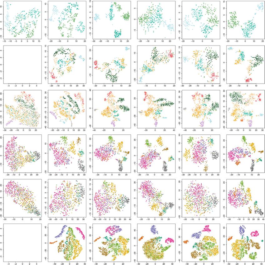
NATURE COMMUNICATIONS | https://doi.org/10.1038/s41467-021-22495-4                                                                        ARTICLE

Fig. 3 Evaluation of the visualization of scCAS data. a The dataset of CLP/LMPP/MPP cells. b The dataset of donor BM0828. c The human bone marrow
dataset. d The mouse forebrain dataset (half). e The mouse forebrain dataset (half) with 25% dropout rate. f The dataset of mouse prefrontal cortex. For all
the datasets, we obtained the latent features from SCALE, Scasat, cisTopic, Cusanovich2018, SnapATAC, and RA3, and then implemented t-SNE for
visualization.

consistently outperformed other methods when the dropout rate                   separation of ACs and OCs (Fig. 3f), and the best overall
varies from 5 to 50% (Fig. 4b and Supplementary Fig. 8).                        clustering performance (Fig. 4a). RA3 also outperformed the
Compared with the baseline methods, RA3 was less affected when                  baseline methods on three other datasets, including mouse
the dropout rate increases, and RA3 still achieved reasonable                   cerebellum and two samples of the mouse whole brain
separation of the cells when dropout rate = 25% (Fig. 3e). This                 (Supplementary Fig. 7).
observation suggests the increased benefit of utilizing reference                   We finally tested the performance on the 10X PBMC dataset.
data when the single-cell dataset has higher degree of sparsity.                We used the previously published dataset of PBMC cells49 to
  We also evaluated the performance on the MCA mouse brain                      construct a pseudo-bulk reference based on the provided cell type
dataset10. We used the complete mouse forebrain dataset30 to                    labels. RA3 consistently outperforms the baseline methods
construct a pseudo-bulk reference. We first look at cells from the               according to the RAGI score (Fig. 4c). In addition, RA3 led to
mouse prefrontal cortex. Cusanovich2018 cannot distinguish                      more compact patterns for marker gene activity (Supplementary
excitatory neurons as previously reported10 (Fig. 3f). We                       Fig. 9).
encountered an error when implementing SCALE on this dataset.                      In all the examples, the results of UMAP visualization are
Scasat achieved a slight improvement over Cusanovich2018 in                     similar to that of t-SNE visualization (Supplementary Fig. 5). We
separating excitatory neurons. cisTopic, SnapATAC, and RA3 all                  further evaluated the stability of clustering performance by
provided better separation of the inhibitory neurons and the                    implementing bootstrap on the datasets in Fig. 4a. To be more
subtypes of excitatory neurons (Fig. 3f). RA3 achieved better                   specific, we generated ten bootstrap samples by random sampling

NATURE COMMUNICATIONS | (2021)12:2177 | https://doi.org/10.1038/s41467-021-22495-4 | www.nature.com/naturecommunications                                  7
ARTICLE                                                                  NATURE COMMUNICATIONS | https://doi.org/10.1038/s41467-021-22495-4

Fig. 4 Assessment of the clustering results. We implemented Louvain clustering on the low-dimensional representation provided by each method to get
the cluster assignments. The cluster assignments for scABC were obtained directly from the model output. a The clustering performance using different
methods evaluated by adjusted mutual information (AMI). The measure of center for the error bars denotes the AMI for different methods. The error bar
denotes the estimated standard error in ten bootstrap samples. b The clustering performance using different methods on the mouse forebrain dataset
(half) at different dropout rates evaluated by AMI. c The clustering performance using different methods on the 10X PBMC dataset evaluated by Residual
Average Gini Index (RAGI) score.

with replacement for each of the dataset. We then performed cell              IDF transformed data as the input; for peak-level analysis (dif-
clustering on the bootstrap samples using different methods. The              ferential peak analysis), we used the raw read counts as part of the
error bars in Fig. 4a represent the standard errors estimated by              input. We selected the top 1000 peaks with the smallest p values
bootstrap. In addition to the indexes of clustering performance,              for each cluster, and then applied chromVAR7 to infer the
we present the clustering tables (Supplementary Fig. 10). RA3                 enriched transcription factor (TF) binding motifs within these
achieved a cleaner separation of the cell types, as the clustering            peaks (Methods). Visualization of the top 50 most variable TF
counts are more concentrated on the diagonals of the clustering               binding motifs is shown (Fig. 5b). Thirty-nine of the top 50 most
tables. To assess the computational efficiency and scalability of              variable TF binding motifs have been implicated in hematopoietic
RA3, we benchmarked the running time usage on datasets of                     development (Supplementary Table 2). Among them, some TF
different sizes. As shown in Supplementary Fig. 11a, RA3 can                  binding motifs are specific to one or two clusters (Fig. 5b), and
scale well with the size of scCAS dataset, especially for large               previous literature further corroborates the role of these TFs/
datasets. The computational time of RA3 on datasets with ~5K,                 motifs in the same cell types that the clusters represent: EBF1,
10K, 20K, and 50K cells are 1.7, 7.5, 16.5, and 17.5 min,                     TCF3, and TCF4 are specific to cluster 7, which corresponds to
respectively. The size of the target scCAS dataset is dominant in             CLP cells29,54,55; JDP2, CEBPB, and CEBPE are specific to cluster
determining the computational time of RA3, and the number of                  6, which corresponds to GMP cells29,56,57; and GATA1::TAL1,
components learned from the reference data has a relatively                   GATA2, and GATA3 are specific to cluster 4, which corresponds
minor effect on the computational time (Supplementary Fig. 11b).              to MEP cells58,59.

RA3 facilitates trajectory inference and motif analysis. Other                Discussion
than data visualization and cell clustering, the output of RA3 can            In this work, we have developed RA3 for the analysis of high-
also be implemented in downstream analyses including trajectory               dimensional and sparse single-cell epigenetic data using a
inference and motif enrichment analysis. We use the cells from                reference-guided approach. RA3 simultaneously models the
donor BM0828 for illustration. We implemented Slingshot52 for                 shared biological variation with reference data and the unique
the trajectory inference, which is suggested in a benchmark                   variation in single-cell data that identifies distinct cell sub-
study53. The inputs for Slingshot include the low-dimensional                 populations by incorporating the spike-and-slab prior. We have
representation provided by RA3 and the cluster labels obtained                shown that the reference data in RA3 can be constructed from
from RA3 + Louvain clustering, and the output for Slingshot is                various sources, including bulk ATAC-seq, bulk DNase-seq, and
the smooth curves representing the estimated cell lineages                    pseudo-bulk chromatin accessibility data, which will facilitate the
(Methods). RA3 with Slingshot revealed the differentiation line-              usage of RA3. We demonstrated that RA3 outperforms baseline
age and the inferred trajectory greatly mimics the hematopoietic              methods in effectively extracting latent features of single cells for
differentiation tree29 (Fig. 5a). We then performed motif                     downstream analyses, including data visualization and cell clus-
enrichment analysis for the clusters identified by RA3 + Louvain               tering. RA3 also facilitates trajectory inference and motif
clustering. Cluster-specific peaks are needed for motif analysis               enrichment analysis for scCAS data. In addition, RA3 is robust
and we identified them by the hypothesis testing procedure in                  and scalable to datasets generated with different profiling tech-
scABC using the raw read counts and the cluster labels provided               nologies, and of diverse sample sizes and dimensions.
by RA3 + Louvain clustering8. Note that for cell-level analysis                  Finally, our modeling framework is flexible and can be exten-
(visualization, clustering, and trajectory inference), we used TF-            ded easily. We can incorporate other types of single-cell profiles

8                 NATURE COMMUNICATIONS | (2021)12:2177 | https://doi.org/10.1038/s41467-021-22495-4 | www.nature.com/naturecommunications
NATURE COMMUNICATIONS | https://doi.org/10.1038/s41467-021-22495-4                                                                                                                         ARTICLE

Fig. 5 Trajectory inference and motif enrichment analysis. a t-SNE visualization of the cells from donor BM0828 and the inferred trajectory with Slingshot
using the output of RA3 and Louvain clustering. The hematopoietic differentiation tree29 is shown on the bottomleft. b The top 50 most variable TF binding
motifs within the cluster-specific peaks for the cells of donor BM0828. The deviations calculated by chromVAR are shown. FACS fluorescent activated cell
sorting.

as reference data to avoid the situation that the cell types in                             Let γj ¼ ½γ1j ; ¼ ; γKj T 2 RK ´ 1 denote a K-dimensional binary latent vector for
scCAS data have not been adequately studied from the epigenetic                         cell j. We assume the following priors for γj and hj:
landscape. Besides, we can also extend our approach to non-linear                          (
projection of scCAS data by incorporating deep neural networks                                 γkj ¼ 1; hkj jγkj  γkj N ð0; 1Þ;                                            k ¼ 1; ¼ ; K 1 ; K 1 þ K 2 þ 1; ¼ ; K

to capture higher level features.                                                              γkj  Bernoulli ðθÞ; hkj jγkj  ð1  γkj ÞN ð0; τ 20 Þ þ γkj N ð0; τ 21 Þ;   k ¼ K 1 þ 1; ¼ ; K 1 þ K 2

                                                                                                                                                                                                                    ð5Þ
Methods                                                                                 Note that for the entries in hj1 and hj3 , the prior specification is the same as that
The model of RA3. We first apply TF-IDF transformation to the read count matrix
                                                                                        in Bayesian PCA, while for the entries in hj2 , we assume the spike-and-slab35,36
in scCAS data. TF-IDF transformation achieves two goals in analyzing scCAS data:
(1) it normalizes for sequencing depth; (2) it upweights peaks/regions that do not      prior with pre-specified parameters τ0 < 1 and τ1 > 1. The spike-and-slab prior is
occur very frequently and downweights prevalent peaks/regions. The peaks/regions        the key that encourages the model to find directions in W2 that separate rare and
that are less frequent in scCAS data tend to represent features that distinguish the    distinct cell types from the other cells, and it will help us to distinguish biological
cell types, and giving these features higher weights improves separation of the cell    variation from technical variation. Therefore, the second component W2 hj2
types (Supplementary Fig. 12). RA3 decomposes the variation in the scCAS data           captures the variation unique in scCAS data that separates distinct and rare cell
after TF-IDF transformation into three components: the shared biological variation      types from the other cells. We note that the sparsity specification on hj is
with the reference data, the unique biological variation in scCAS data, and other       different from that in sparse PCA61, where W is assumed to be sparse for
variations. Aside from the three components, RA3 also includes a term for known         variable selection. The third component W3 hj3 models other variations such as
covariates.                                                                             technical variation. We believe that hj1 and hj2 more likely represent the
    Consider the random vector yj 2 Rp ´ 1 , which represents the observed p            biological variation, and thus we use the learned hj1 and hj2 as the low-
features/regions for the jth cell among n cells in total. Borrowing the general         dimensional representation for cell j. The parameter θ is pre-specified to
framework of probabilistic PCA33, RA3 models yj as the following:                       determine the size of the rare cell types. In practice, we set the parameters τ0 =
                                                                                        0.9, τ1 = 5, and θ = 0.1. We set both K2 and K3 equal to 5, and set K1 equal to the
                               yj jλj  N p ðλj ; σ 2 Ip Þ;                       ð1Þ   number of reference bulk/pseudo-bulk samples, as we used all the principal
                                                                                        components (PCs) in the reference data. When more than 30 bulk samples are
                                                                                        used to construct the reference, we retained the loading matrix of the first 30 PCs
                           λj ¼ βxj þ Whj ; λj 2 Rp ´ 1 ;                         ð2Þ   learned from the reference data when implementing RA3. The performance of
                                                                                        RA3 is robust to the choice of τ0, τ1, θ, K2, and K3 (Supplementary Figs. 13 and
where xj 2 Rq ´ 1 represents q known covariates, including the intercept and other      14) and the number of PCs learned from the reference data (Supplementary
                                                                                        Fig. 15). In practice, we found that as long as K1 passes certain value, RA3
variables, such as the labels of donors or batches, and β 2 Rp ´ q represents the
                                                                                        performs well and stable when it further increases. The reason is that the prior
unknown coefficients for xj. The variables W 2 Rp ´ K and hj 2 RK ´ 1 are latent         on h⋅1 has a shrinkage effect, the variations of h⋅1 for the irrelevant projection
variables: the columns in W have similar interpretation as the projection vectors in    vectors are small and will be further shrunk toward 0. We set the default value of
PCA, and hj can be interpreted as the low-dimensional representation of yj. We          K1 to be capped at 30. The value of K1 has a minor effect on the computational
further decomposes the term Whj into three components:                                  time of RA3, compared to the scale of the target scCAS dataset (Supplementary
                                                                                        Fig. 11b).
                         Whj ¼ W1 hj1 þ W2 hj2 þ W3 hj3 ;                         ð3Þ
                                                                                        Model fitting and parameter estimation. Given the observed scCAS matrix Y 2
where the dimensions are W1 2 Rp ´ K 1 , W2 2 Rp ´ K 2 , W3 2 Rp ´ K 3 , hj1 2          Rp ´ n after TF-IDF transformation and                                         X 2 Rq ´ n , we
                                                                                                                                         the matrix
                                                                                                                                                  ofKcovariates
                                                                                                                                                             ´n
RK 1 ´ 1 , hj2 2 RK 2 ´ 1 , hj3 2 RK 3 ´ 1 . So we have W = [W1 W2 W3] and hj ¼         treat the latent variable matrix H ¼ h1 ; ¼ ; hn 2 R                    as missing data, and use
                 T
                       h           iT            h        iT                            the expectation-maximization (EM) algorithm to estimate the model parameters
½hTj1 hTj2 hTj3  ¼ hTj1 hT     j    with hj ≜ hTj2 hTj3 .                            Θ = (Γ, A, W*, β, σ), where Γ ¼ ½γ1 ; ¼ ; γn  2 RK ´ n , A ¼ diagðαK 1 þ1 ; ¼ ; αK Þ 2

    We set W1 to be equal to the K1 projection vectors learned from PCA on the          RðK 2 þK 3 Þ ´ ðK 2 þK 3 Þ and W ¼ W2 W3 ¼ ½wK 1 þ1 ; ¼ ; wK  2 Rp ´ ðK 2 þK 3 Þ . For
reference data, so the first component W1 hj1 utilizes prior information from the                                                                                                     T
                                                                                        simplicity of the derivation that will follow, we also write H ¼ HT1 HT2 HT3 ,
reference data and captures the shared biological variation among scCAS data and                              K1 ´ n          K2 ´ n              K3 ´ n
the reference data.                                                                     where H1 2 R                 , H2 2 R        , and H3 2 R        , corresponding to the
                                                                                                                                                                            T
    For the columns in W2 and W3, the prior specification is similar to that in          decomposition of variation introduced previously, and hj ¼ ½hTj2 hTj3  ,
Bayesian PCA60:                                                                         H ¼ ½HT2 HT3  .
                                                                                                                  T

                                                                                            In the expectation step (E-step), given the parameters estimated in the previous
                   wk  N p ð0; α1
                                 k Ip Þ; for k ¼ K 1 þ 1; ¼ ; K;                  ð4Þ   iteration Θt−1, the posterior distribution of hj is
where hyper-parameters α ¼ fαK 1 þ1 ; ¼ ; αK g are precision parameters that
                                                                                                                                   hj jy j ; xj ; Θt1  N K ð^    ^ j Þ;
                                                                                                                                                              μj ; Σ                                                ð6Þ
controls the inverse variance of the corresponding wk, for k = K1 + 1, …, K.

NATURE COMMUNICATIONS | (2021)12:2177 | https://doi.org/10.1038/s41467-021-22495-4 | www.nature.com/naturecommunications                                                                                             9
ARTICLE NATURE COMMUNICATIONS | https://doi.org/10.1038/s41467-021-22495-4
1 To initialize σ, we first obtain the residual by subtracting from Y the projection
^ j ¼ ðσ 2 WT W þ D1
where Σ ^ j , and
^j ¼ σ 2 ðyj βxj ÞT WΣ
j Þ , μ
onto the column space of W1 and VR, and we then initialize σ as the standard
... ..
Dj ¼ I K 1 0ð1 γðK 1 þ1Þj Þτ 20 þ γðK 1 þ1Þj τ 21 0.... . .....0 ð1 γðK 1 þK 2 Þj Þτ 20 þ γðK 1 þK 2 Þj τ 21 0 IK 3 2 RKdeviation
´K
: of the residual. We initialize A with the identity matrix, and β with zeros.
We initialize γkj with 0 for k = K1 + 1, …, K1 + K2 and 1 for other k. W3 is initi-
ð7Þ alized by a random matrix with elements distributed as standard Gaussian
Based on the posterior distribution, we compute the following expectations: distribution.
(
^Tj ;
Eðhj Þ ¼ μ Datasets and data processing
ð8Þ
^j:
Eðhj hTj Þ ¼ Eðhj ÞEðhj ÞT þ Σ Datasets. The human bone marrow dataset contains single-cell chromatin acces-
sibility profiles across ten populations of immunophenotypically defined human
In the maximization step (M-step), we maximize the expected value of the hematopoietic cell types from seven donors29. The GM/HEK and GM/HL datasets
complete log-likelihood with respect to Θ. The corresponding objective function is are mixtures of the cell lines GM12878/HEK293T and GM12878/HL-60,
Q ¼ EHjY;θ ðlog PðYjW; H; X; A; βÞ þ log PðWjAÞ þ log PðHjΓÞ þ log PðΓÞÞ correspondingly5. The InSilico mixture dataset was constructed by computationally
np 1 h i combining scCAS datasets from H1, K562, GM12878, TF-1, HL-60, and BJ cell
¼ log σ 2 EHjY;θ trace σ 2 ðY βXÞT ðY βXÞ 2σ 2 ðY βXÞT WH þ σ 2 ðWHÞT WH
2 2 lines4. The mouse forebrain dataset was generated from the forebrain tissue from
K 1 1 an 8-week-old adult mouse (postnatal day 56) by single-nucleus ATAC-seq30. The
þ ∑ log jα1 k I p j αk w k w k
T
k¼K 1 þ1 2 2 MCA mouse brain dataset was generated from the prefrontal cortex, cerebellum,
1 n K 2 and two samples from the whole brain of 8-week-old mice using sciATAC-seq,
∑ ∑ E hj hTj φ γkj log φ γkj
2 j¼1 k¼1 kk which is a combinatorial indexing assay10. The 10X PBMC dataset produced by
n h i 10X Chromium Single Cell ATAC-seq was generated from PBMC from a
þ∑ ∑ γkj log θ þ ð1 γkj Þlog ð1 θÞ ;
j¼1 k¼K 1 þ1; ¼ ;K 1 þK 2 healthy donor.
ð9Þ
Data preprocessing. To reduce the noise level, we selected peaks/regions that have at
ð1 γkj Þτ 2 2
0 þ γkj τ 1 ; k ¼ K 1 þ 1; ¼ ; K 1 þ K 2
where φðγkj Þ ¼ , least one read count in at least 3% of the cells in the scCAS count matrix. Similar to
1; k ¼ 1; ¼ ; K 1 ; K 1 þ K 2 þ 1; ¼ ; K Cusanovich et al.10, we performed TF-IDF transformation to normalize the scCAS
and Eðhj hj Þkk is the kth diagonal element of matrix Eðhj hj Þ.
T T
count matrix before implementing our model: we first weighted all the regions in
The optimization problem can be solved by the iterative conditional mode individual cells by the term frequency, which is the total number of accessible
algorithm: in each step, we search for the mode of one group of variables, fixing the regions in that cell, and then multiplied these weighted matrix by the logarithm of
other variables. To update A, W, β and σ, we use the following formulas derived by inverse document frequency, which is the inverse frequency of each region to be
setting the gradients to zero: accessible across all cells.
p
αk ¼ T ; for k ¼ K 1 þ 1; ¼ ; K ð10Þ Downsampling procedure. We randomly dropped out the non-zero entries in the
wk wk
data matrix to zero with probability equal to the dropout rate.
n 1
W ¼ ðY βX W1 H1 ÞEðH ÞT ∑ E hj hT
j þ σ2A ; ð11Þ Construction of reference
j¼1
Manually curated bulk reference. For the human bone marrow dataset, we used
1 bulk ATAC-seq data of HSC, MPP, LMPP, CMP, GMP, MEP, Mono, CD4, CD8,
β ¼ ðY WHÞXT ðXXT Þ ; ð12Þ NK, NKT, B, CLP, Ery, UNK, pDC, and Mega cells provided by Buenrostro et al.29
h i as the reference data in RA3. To construct the reference for the GM/HEK, GM/HL,
∑nj¼1 ðy j βxj ÞT ðyj βxj Þ 2ðyj βxj ÞT WEðhj Þ þ traceðEðhj hTj ÞWT WÞ and InSilico mixture datasets, we first downloaded BAM files of bulk DNase-seq
σ ¼
2
: samples with relevant biological context from ENCODE15,16: GM12878 and
pn HEK293T cell lines for the GM/HEK dataset, GM12878 and HL-60 cell lines for
ð13Þ the GM/HL dataset, and H1, K562, GM12878, HL-60, and BJ cell lines for the
The variable Γ is updated element-wise by choosing γkj ∈ {0, 1} that maximizes InSilico mixture dataset. We then counted the reads that fall into the regions of
scCAS data for the bulk samples to form a count matrix that has same features/
1 2 1 regions as the target single-cell data. We finally obtained the reference data through
f γkj ðγkj Þ ¼ Eðhj hTj Þkk φðγkj Þ þ logφðγkj Þ þ γkj logθ þ ð1 γkj Þlogð1 θÞ;
2 2 scaling the count matrix by total mapped reads of each bulk sample.
ð14Þ
where φ(γkj) is defined as OPENANNO. The webserver OPENANNO31 provides a convenient and straight-
( forward approach to construct the reference. OPENANNO can annotate chro-
φðγkj Þ ¼ 1; k ¼ 1; ¼ ; K 1 ; K 1 þ K 2 þ 1; ¼ ; K matin accessibility of arbitrary genomic regions by the normalized number of reads
ð15Þ that fall into the regions using BAM files, or the normalized number of peaks that
φðγkj Þ ¼ ð1 γkj Þτ 2 2
0 þ γkj τ 1 ; k ¼ K 1 þ 1; ¼ ; K 1 þ K 2 :
overlap with the regions using BED files. After submitting the peak file in scCAS
We iteratively repeat the above E-step and M-step until convergence. E(H1) and data to the webserver, OPENANNO computes the accessibility of the single-cell
E(H2) obtained from the last iteration of the EM algorithm are used for peaks across 199 cell lines, 48 tissues, and 11 systems based on 871 DNase-seq
downstream analyses, including data visualization, cell clustering, trajectory samples from ENCODE. When more than 30 bulk samples are used to construct
inference, and motif analysis. We implement an optional post-processing step for E the reference, we retained the loading matrix of the first 30 PCs learned from the
(H2). We first perform the one-sample t-test for each row of the estimate of E(H2) reference data when implementing RA3.
obtained from the final iteration in EM algorithm, and test if its distribution has a
zero mean. Here we do not include the multiple testing correction procedure, as the Pseudo-bulk reference by aggregrating single cells. Given that it can be difficult to
number of rows for testing (K2) is usually small. The rows that cannot reject the obtain the bulk samples for certain cell populations, we can alternatively construct
null hypothesis under the 0.05 significant level would be discarded for following pseudo-bulk reference data by aggregrating single cells of the same type/cluster. To
analysis. We then truncate the values in each remaining row of E(H2) by the 5th address the bias of the difference in cell type abundance in constructing the
and 95th percentile. The purpose of the post-processing step is to alleviate the effect reference, we took average (instead of taking sum) for each peak over single cells of
of noisy cells with low sequencing depth. In practice, some components in H2 may the same type/cluster. When the peaks do not match between the target single-cell
capture very few cells (NATURE COMMUNICATIONS | https://doi.org/10.1038/s41467-021-22495-4 ARTICLE
the identified cell subpopulation. We then submitted these peaks to the GREAT37 for the expected agreement by chance, and it is calculated as follows:
server with a whole genome background and the default parameter settings to
nij xi y N
identify significant pathways associated with the peaks and thus obtain functional ∑ij ∑i ∑j j =
insight on the identified cell subpopulation. We note that our analysis with GREAT 2 2 2 2
ARI ¼ :
does not require knowing the cell labels. xi yj xi yj N
2 ∑i þ ∑j ∑i ∑j =
1
2 2 2 2 2
Trajectory inference. We adopted Slingshot52 for trajectory inference, which is the Both NMI and AMI are based on mutual information (MI), which assesses the
best method of single-cell trajectory inference for tree-shaped trajectories as sug- similarity between the obtained clusters and the cell type labels. NMI scales MI to
gested in a benchmark study53. With the default parameter settings, we used the be between 0 and 1, and it is calculated as follows:
getLineages function to learn cluster relationships using the low-dimensional
representation provided by RA3 and the cluster labels obtained from RA3 + MI ðP; TÞ
NMI ¼ pffiffiffiffiffiffiffiffiffiffiffiffiffiffiffiffiffiffiffiffiffi ;
Louvain clustering, and then constructed smooth curves representing the estimated HðPÞHðTÞ
cell lineages using the getCurves function. We then used the embedCurves function
to map the curves to the two-dimensional t-SNE space for visualization. where H(⋅) is the entropy function.
AMI adjusts MI by considering the expected value under random clustering,
and it is calculated as follows:
Motif enrichment analysis. With the cluster labels obtained from RA3 + Louvain
clustering, we identified the cluster-specific peaks by implementing the hypothesis MI ðP; TÞ E½ MI ðP; TÞ
AMI ¼ ;
testing procedure in scABC8 on the raw read counts. We selected the top 1000 avg½HðPÞ; HðTÞ E½ MI ðP; TÞ
peaks with smallest p values for each cluster, and then performed TF binding motif
where E(⋅) denotes the expectation function.
enrichment within these peaks using chromVAR7.
The homogeneity score assesses whether the obtained clusters contain only
cells of the same cell type, and it is equal to 1 if all the cells within the same
cluster correspond to the same cell type. The homogeneity score is computed as
Discussion on the Gaussian assumption. TF-IDF transformation is necessary for follows:
better separation of the cells. After TF-IDF transformation, the data matrix is no HðTjPÞ
longer discrete and becomes continuous. Gaussian distribution is commonly used Homogeneity ¼ 1 ;
HðTÞ
to model continuous data and it has high computational efficiency given its con-
jugacy in our model. Computation is an important concern given the scale of the where H(T∣P) indicates the uncertainty of true labels based on the knowledge of
datasets. We used the Kolmogorov–Smirnov (KS) test to test the normality of predicted assignments.
individual peaks within each cell type after TF-IDF transformation. It is a one- A comparison of ARI, NMI, and AMI was presented in65. ARI is preferred
dimensional KS test as testing high-dimensional normality is not feasible. It when there are large equal-sized clusters65. AMI is theoretically preferred to NMI,
showed that up to 90% of the one-dimensional tests have been rejected, which even though NMI is also very commonly used. AMI is preferred when the sizes of
suggests that TF-IDF transformed data are not normally distributed. However, clusters are unbalanced and when there are small clusters65.
given the good performance in all our examples, we think that the Gaussian We adopted the RAGI score6 to evaluate the clustering performance for the
assumption is robust for cell-level analysis, including visualization, clustering, and 10X PBMC dataset, since no cell type labels are provided in this dataset. The
lineage reconstruction. For feature-level analysis, including differential peak ana- RAGI score calculates the difference between (a) the variability of marker gene
lysis, the raw read counts should be used. We implemented scABC to detect accessibility across clusters and (b) the variability of housekeeping gene
differential peaks, using the raw read counts and the cluster labels obtained by RA3 accessibility across clusters. More specifically, we first used the Gene Scoring
+ Louvain clustering. method66 to summarize the accessibility for each gene in each cell. We then
computed the mean gene score among cells within each cluster, and computed
the Gini index67 for each marker gene48 based on these mean gene scores. We
use a set of annotated housekeeping genes reported in https://m.tau.ac.il/elieis/
Baseline methods. We compared the performance of RA3 with six baseline HKG/HK_genes.txt. The Gini index for each housekeeping gene is calculated
methods (using their default parameters), including scABC8, SCALE13, Scasat11, similarly as that for the marker gene. We take average of the Gini indexes within
cisTopic9, Cusanovich20185,10, and SnapATAC12. Source code for implementing the set of marker genes and the set of housekeeping genes, respectively. Last we
the baseline methods was obtained from a benchmark study6. We set uniform obtain the RAGI score by calculating the difference in the average Gini indexes
random seeds in all experiments to ensure the reproducibility of results. Similar to in these two sets of genes. Intuitively, a good clustering result should contain
SCALE, we applied all the baseline methods to reduce the scATAC-seq data to ten clusters that are enriched for accessibility of the marker genes, and each marker
dimensions for downstream visualization and clustering. To ensure data con- gene should be highly accessible in only one or a few clusters. A larger RAGI
sistency, we disabled the parameters for filtering peaks and cells in SCALE, and we score indicates a better separation of the clusters.
used the peaks in single-cell data instead of binning the genome into fixed-size
windows when implementing SnapATAC.
Reporting summary. Further information on research design is available in the Nature
Research Reporting Summary linked to this article.
Visualization and clustering
Visualization. We first obtained the low-dimensional representation provided by Data availability
each method. To further reduce the dimension to two, we then implemented t-SNE The human bone marrow dataset and the corresponding reference ATAC-seq data were
using the R package Rtsne34, and UMAP using the R package UMAP50. retrieved from NCBI Gene Expression Omnibus (GEO) with the accession number
GSE96772. Single-cell data of the GM/HEK and GM/HL datasets are available at GEO
GSE68103. The InSilico mixture dataset was collected from GEO with the accession
Clustering. We first obtained the low-dimensional representation provided by each
method except for scABC, and then implemented Louvain clustering62–64 by number GSE65360. BAM files of the reference data for GM/HEK, GM/HL, and InSilico
scanpy64, which is a community detection-based clustering method. The cluster mixture datasets were obtained from ENCODE with the following accession number:
assignments for scABC were directly obtained from the model output. We ENCFF774HUB, ENCFF775ZJX, and ENCFF783ZLL for the GM/HEK dataset;
implemented binary search to tune the resolution parameter in Louvain clustering ENCFF783ZLL, ENCFF775ZJX, ENCFF746RUG, and ENCFF328JJT for the GM/HL
to make the number of clusters and the number of cell types as close as possible6. dataset; and ENCFF328JJT, ENCFF826DJP, ENCFF923SKV, ENCFF775ZJX, and
We used eight as the number of expected cell populations for the 10X PBMC ENCFF949CIK for the InSilico mixture dataset. The mouse forebrain dataset can be
dataset. accessed in GEO with the accession number GSE100033. The MCA mouse brain dataset
is available at http://atlas.gs.washington.edu/mouse-atac. The 10X PBMC dataset is
available at https://support.10xgenomics.com/single-cell-atac/datasets. The reference
data of fresh PBMCs were downloaded from GEO with the accession number
Metrics for evaluation of clustering results. We evaluated the clustering GSE129785. A reporting summary for this article is available as a Supplementary
methods based on ARI, NMI, AMI, and homogeneity scores. Information file.
Let T denote the known ground-truth labels of cells, P denote the predicted
clustering assignments, N denote the total number of single cells, xi denote the
number of cells assigned to the ith cluster of P, yj denote the number of cells that Code availability
belong to the jth unique label of T, and nij denote the number of overlapping cells The RA3 R package with a detailed tutorial is freely available at https://github.com/
between the ith cluster and the jth unique label. Rand index (RI) represents the cuhklinlab/RA3 (https://doi.org/10.5281/zenodo.4581063)68. The source code for
probability that the obtained clusters and the provided cell type labels will agree on reproduction is available at https://github.com/cuhklinlab/RA3_source (https://doi.org/
a randomly chosen pair of cells. ARI is an adjusted version of RI, where it adjusts 10.5281/zenodo.4581077).
NATURE COMMUNICATIONS | (2021)12:2177 | https://doi.org/10.1038/s41467-021-22495-4 | www.nature.com/naturecommunications 11You can also read