Credal decision tree based novel ensemble models for spatial assessment of gully erosion and sustainable management
←
→
Page content transcription
If your browser does not render page correctly, please read the page content below
www.nature.com/scientificreports
OPEN Credal decision tree based novel
ensemble models for spatial
assessment of gully erosion
and sustainable management
Alireza Arabameri1*, Nitheshnirmal Sadhasivam2,3, Hamza Turabieh4, Majdi Mafarja5,
Fatemeh Rezaie6,7, Subodh Chandra Pal8 & M. Santosh9,10
We introduce novel hybrid ensemble models in gully erosion susceptibility mapping (GESM) through
a case study in the Bastam sedimentary plain of Northern Iran. Four new ensemble models including
credal decision tree-bagging (CDT-BA), credal decision tree-dagging (CDT-DA), credal decision tree-
rotation forest (CDT-RF), and credal decision tree-alternative decision tree (CDT-ADTree) are employed
for mapping the gully erosion susceptibility (GES) with the help of 14 predictor factors and 293 gully
locations. The relative significance of GECFs in modelling GES is assessed by random forest algorithm.
Two cut-off-independent (area under success rate curve and area under predictor rate curve) and six
cut-off-dependent metrics (accuracy, sensitivity, specificity, F-score, odd ratio and Cohen Kappa)
were utilized based on both calibration as well as testing dataset. Drainage density, distance to road,
rainfall and NDVI were found to be the most influencing predictor variables for GESM. The CDT-RF
(AUSRC = 0.942, AUPRC = 0.945, accuracy = 0.869, specificity = 0.875, sensitivity = 0.864, RMSE = 0.488,
F-score = 0.869 and Cohen’s Kappa = 0.305) was found to be the most robust model which showcased
outstanding predictive accuracy in mapping GES. Our study shows that the GESM can be utilized for
conserving soil resources and for controlling future gully erosion.
The agrarian economy is faced with the challenge of maintaining food security despite the increasing global
population, and in tackling serious threats, including a decline in food productivity, climate change and lack of
freshwater resources1. Better conservation of soil resources, which necessitates control on soil erosion, is one of
the most significant aspects in improving land productivity2. Soil is a finite resource and plays a major role in
human existence as the source of more than 99% of our nourishment3. Among several triggering agents for soil
erosion, water plays a major r ole2. It has been assessed that soil erosion causes a yearly global GDP loss of almost
$8 billion2. Iran is among the many countries that is worst affected by soil erosion, with an annual soil loss of
about 32 tons per hectare from farmlands3. The most adverse type of water-triggered soil erosion that largely
deteriorates the agricultural lands of Iran is gully erosion (GE)2.
Gullies can be temporary (ephemeral) or permanent (classical) where the latter is larger than the former9.
In places where intense flow intersects earth bank, bank gullies can also occur. In general, gullies represent
incised deep linear geomorphological features, varying in depth between 0.5 and 30 m 4. Development of gullies
5
mostly occur in loess s oil . There are two phases in gully development, one is initiation of gully which occurs
in smaller timespan and the other is the stable sediment transportation p hase2. GE is created by running water,
6
mass-wasting and subterranean process that erodes soil particles , and results in numerous onsite and offsite
1
Department of Geomorphology, Tarbiat Modares University, Jalal Ale Ahmad Highway, 9821 Tehran,
Iran. 2Faculty of Geo‑Information Science and Earth Observation (ITC), University of Twente, Enschede, The
Netherlands. 3Department of Geography, Bharathidasan University, Tiruchirappalli, Tamil Nadu 620024,
India. 4Department of Information Technology, College of Computers and Information Technology, Taif
University, P.O. Box11099, Taif 21944, Saudi Arabia. 5Department of Computer Science, Birzeit University, Birzeit,
Palestine. 6Geoscience Platform Research Division, Korea Institute of Geoscience and Mineral Resources (KIGAM),
124, Gwahak‑ro Yuseong‑gu, Daejeon 34132, Republic of Korea. 7Korea University of Science and Technology,
217 Gajeong‑roYuseong‑gu, Daejeon 34113, Republic of Korea. 8Department of Geography, The University of
Burdwan, Bardhaman, West Bengal 713104, India. 9School of Earth Sciences and Resources, China University of
Geosciences Beijing, Beijing, China. 10Department of Earth Sciences, University of Adelaide, Adelaide, South
Australia, Australia. *email: Alireza.ameri91@yahoo.com
Scientific Reports | (2021) 11:3147 | https://doi.org/10.1038/s41598-021-82527-3 1
Vol.:(0123456789)
www.nature.com/scientificreports/
effects including land degradation, soil fertility loss, and accumulation of sediments, landslide, flooding and
decline of water q uality5–7. GE not only causes environmental deterioration but also immensely impacts the
socio-economic aspects8. Previous studies have shown the main role of GE in transporting sediments from
upper region of the c atchments9. Thus, a precise evaluation of gully erosion susceptibility (GSE) is an essential
requirement for planners and decision-makers in controlling the subsequent problems of GE and for a sustain-
able management of soil resources3.
Various factors including topographic, geologic, hydrologic, environmental, climatic and anthropogenic
E10–12. Rahmati et al.10 reported that drainage density, distance to stream and
activities, instigate the process of G
land use also play a vital role in triggering GE. Zhao et al.12 noted that GE is mostly initiated by natural processes
rather than anthropogenic activities and that the density of gullies is reliant on the intensity of vegetation cover
and topographic features.
Most of the physically based models reported in earlier studies of gully erosion were not aimed at predicting
the gully hotspots, but focused on quantifying the erosion rates11. For predicting the evolution of gullies, dynamic
and static models have been utilized previously based on the development phase of the g ully2. However, both
these models require different erosion factors which are hard to quantify for a large area. Thus, for the gully ero-
sion susceptibility mapping (GESM), researchers utilized various models such as knowledge based, statistical and
machine learning algorithms (MLAs) coupled with geographical information system (GIS) and remote sensing
(RS)13. The knowledge-based models include multi-criteria decision-making models (MCDM) that involve the
decision made by experts to prepare the GESM. Even though there are more than nearly 20 MCDM models
available, the derived factor weights based on these models are still subjective14. Several bivariate and multivari-
ate statistical models such as frequency ratio15, logistic regression16, weights of evidence17, and certainty factor18
also used for generating GESM. The benefit of employing statistical models is that various types of predictor
variable can be easily accommodated in the e valuation13. The disadvantages of using simple bivariate models are
that these could be ad-hoc processes owing to the poor probability distribution that the bivariate models depend
on15. In the case of parametric multivariate models, the resultant spatial maps become smoother than in MLAs,
and provide more elaborate maps of GES19.
Various MLAs including random forest20, logistic model tree (LMT)13, support vector machine(SVM)21,
naive Bayes tree (NBT)13, multivariate adaptive regression spline (MARS)22, generalized linear model (GLM)23,
artificial neural network (ANN)24, boosted regression tree (BRT)22, mixture discriminant analysis (MDA)18,
classification and regression trees (CART)25, and functional data analysis14 are commonly utilized for the crea-
tion of GESM. The MLAs exhibit a superior predictive accuracy than statistical models in GESM owing to
their advantage in handling huge datasets and potential ability in assessing the intricate relationship between
dependent and predictor variables26. Performance of individual models can be enhanced using hybrid ensemble
methods27,28. Hybrid ensemble methods outperform the forecast preciseness of individual MLA29. Arabameri
et al.30 showed that meta-classifiers increase the classification accuracy of the base classifiers in gully erosion
susceptibility modelling. It is essential to test a novel base classifier using different meta-classifiers11. Chowdhuri
et al.31 reported high predictive accuracy of hybrid ensemble BRT-bagging (BA) algorithm in comparison with
the individual BRT and bagging algorithms. Similar results were displayed by Roy and S aha32 in their study in
which the authors reported Multilayer perceptron neural network-dagging (DA) ensemble.
In this study, we propose novel hybrid ensemble models for mapping GES based on a case study on the Bastam
sedimentary plain of Northern Iran. Apart from individual credal decision trees (CDT) model, we integrated four
meta-classifiers including bagging, dagging, rotation forest (RF) and alternating decision tree (ADTree) with a
base-classifier, i.e., the CDT for GESM. To our knowledge, no previous study has employed the CDT both as a
base classifier in a hybrid ensemble model and as an individual model for predicting the GES. The four hybrid
ensemble models, namely CDT-BA, CDT-DA, CDT-RF and CDT-ADTree along with CDT were compared, and
the best model is identified. The significance of the gully erosion conditioning factors (GECFs) for mapping GES
is evaluated using the random forest model. The predictor variables used in this work for forecasting GES include
clay content, bulk density, elevation, distance to road, distance to stream, drainage density, lithology, land use/
land cover (LU/LC), normalized difference vegetation index (NDVI), rainfall, terrain rugged index (TRI), slit
content, slope degree, and topography wetness index (TWI).
Results
Outcome of multi‑collinearity test. The values of VIF and tol used for testing the multi-collinearity
among GECFs are given in Table 2. The NDVI shows minimum VIF value of 1.099 and TRI has maximum
VIF value of 4.184 and, since the tol is the reciprocal of VIF, the NDVI and TRI acquired the maximum (0.910)
and minimum tol value (0.239). The VIF and tol values of GECFs from Table 1 indicate that there is no linear
dependency among the GECFs and confirms that all the selected fourteen GECFs can be utilized for the genera-
tion of GESMs (Table 2).
Relative significance of GECFs. This study employed the random forest algorithm for assessing the sig-
nificance of GECFs in mapping GES. The confusion matrix created by random forest with gully presence (1) and
gully absence (0) information is provided in Table 3. The algorithm generated an OOB error of 6.54%, which
infers that the precision of the predicted values is equivalent to 93.46%. From Table 2, it can be observed that
among 201 non-gully locations, 190 were identified as non-gully locations and 11 were determined to be gully
locations. On the other hand, among 212 gully locations, 196 were predicted as gully locations while 16 were
identified as non-gully locations. The outcome of the relative significance of GECFs assessed using the mean
decrease in accuracy and mean decrease Gini of the random forest algorithm is provided in Table 3. The GECFs
including drainage density (29.10), distance to road (24.72), rainfall (12.86) and NDVI (12.74) exhibited high
Scientific Reports | (2021) 11:3147 | https://doi.org/10.1038/s41598-021-82527-3 2
Vol:.(1234567890)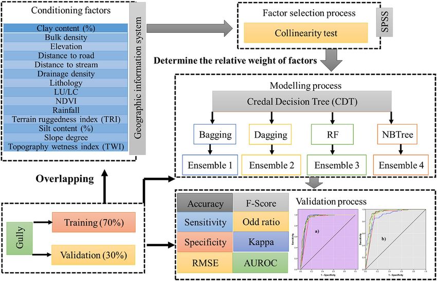
www.nature.com/scientificreports/

                                                                   Collinearity
                                                                   Statistics
                                   Conditioning factors            Tolerance      VIF
                                   Landuse                         0.544          1.838
                                   Lithology                       0.885          1.130
                                   Elevation                       0.304          3.290
                                   TWI                             0.817          1.224
                                   Rainfall (mm)                   0.260          3.847
                                   Content of silt (%)             0.366          2.736
                                   Slope degree                    0.272          3.676
                                   TRI                             0.239          4.184
                                   Bulk density                    0.455          2.196
                                   Content of clay (%)             0.713          1.403
                                   Distance to road (m)            0.459          2.177
                                   Distance to stream (m)          0.717          1.394
                                   Drainage density (km/km2)       0.659          1.518
                                   NDVI                            0.910          1.099

                                  Table 1.  Multi-Collinearity analysis of the gully conditioning factors.

                                            0      1
                                   0        190    16
                                   1        11     196

                                  Table 2.  Confusion matrix from the RF model (0 = no gully, 1 = gully).

                                   Factor                 Relative weight   Factor               Relative weight
                                   Drainage density       29.10             Lithology            2.63
                                   Distance to road       24.72             TWI                  5.79
                                   Rainfall               12.86             Bulk density         6.27
                                   NDVI                   12.74             Slope degree         9.48
                                   Silt content (%)        6.57             Clay content (%)     2.59
                                   Elevation               9.05             LU/LC                0.94
                                   TRI                     5.55             Distance to stream   2.51

                                  Table 3.  Relative influence of effective conditioning factors in the random forest model.

                                  significance in influencing GE while slope degree (9.48), elevation (9.05), silt content (6.57), bulk density (6.27),
                                  TWI (5.79), TRI (5.55) displayed moderate control over the process, but factors such as lithology, clay content,
                                  distance to stream and LU/LC showed the least significance in the initiation of GE.

                                  Gully erosion susceptibility mapping (GESM). Observations on the presence or absence of gully com-
                                  prising the values of GECFs were provided as inputs for MLAs in R 3.6.0 to generate the GESMs. The GES index
                                  output generated by the CDT, CDT-DA, CDT-ADTree, CDT-BA and CDT-RF models (Fig. 1a–e, respectively)
                                  were exported to ArcGIS 10.5 and categorized into very low, low, moderate, high and very high susceptibility
                                  classes with the help of natural breaks technique.

                                  Credal decision tree (CDT).          The GESM produced by CDT shows that 51.16% and 1.67% of pixels come
                                  under very high and high GES zone, whereas moderate, low and very low GES zone covers 4.52%, 10.95% and
                                  31.70% of pixels in Bastam sedimentary plain, respectively (Fig. 1a). The total number of pixels present in each
                                  GES classes of CDT is provided in Table 4. The number of gully pixels in the very high, high, moderate, low and
                                  very low GES zones are279, 4, 3, 2, and 5 whereas the percentage of gully pixels in the same order of susceptibility
                                  classes was 95.22%, 1.37%, 1.02%, 0.68% and 1.71%, respectively.

                                  CDT‑dagging (DA). The GESM from CDT-DA model shows about 32.55%, 17.06%, 9.10%, 22.10% and
                                  19.19% of pixels in the study area that falls under very high, high, moderate, low and very low GES class, respec-

Scientific Reports |   (2021) 11:3147 |                      https://doi.org/10.1038/s41598-021-82527-3                                              3

                                                                                                                                                Vol.:(0123456789)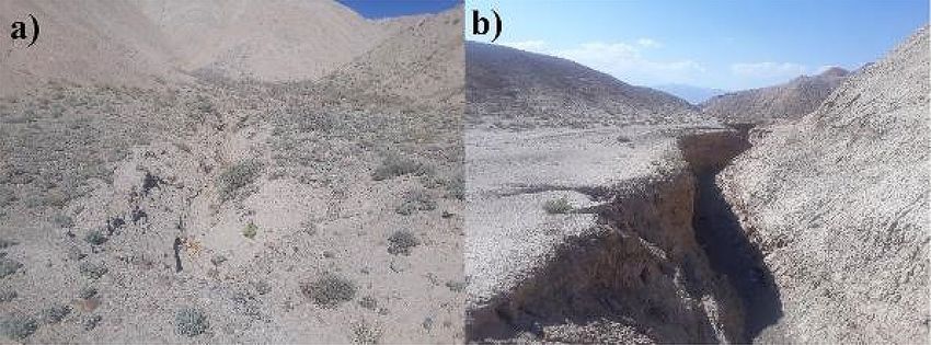
www.nature.com/scientificreports/
Figure 1. Gully erosion susceptibility mapping using (a) credal decision tree (CDT), (b) CDT-Dagging, (c)
CDT-ADTree, (d) CDT-Bagging, (e) CDT-rotational forest (RF). ArcGIS 10.5 software was used for preparing
this map (https://desktop.arcgis.com/en/).
Scientific Reports | (2021) 11:3147 | https://doi.org/10.1038/s41598-021-82527-3 4
Vol:.(1234567890)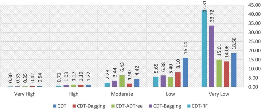
www.nature.com/scientificreports/

                                   Model          Class        Number of gully pixels   Percentage of class pixels (%)   Percentage of gully pixels (%)
                                                  Very low     4                        19.19                             1.37
                                                  Low          8                        22.10                             2.73
                                   CDT-Dagging    Moderate     14                        9.10                             4.78
                                                  High         42                       17.06                            14.33
                                                  Very high    225                      32.55                            76.79
                                                  Very low     5                        31.70                             1.71
                                                  Low          2                        10.95                             0.68
                                   CDT            Moderate     3                         4.52                             1.02
                                                  High         4                         1.67                             1.37
                                                  Very high    279                      51.16                            95.22
                                                  Very low     3                        15.37                             1.02
                                                  Low          8                        14.74                             2.73
                                   CDT-ADTree     Moderate     10                       21.93                             3.41
                                                  High         49                       21.20                            16.72
                                                  Very high    223                      26.75                            76.11
                                                  Very low     2                        23.02                             0.68
                                                  Low          9                        19.59                             3.07
                                   CDT-Bagging    Moderate     14                       16.43                             4.78
                                                  High         45                       15.85                            15.36
                                                  Very high    223                      25.11                            76.11
                                                  Very low     2                        28.88                             0.68
                                                  Low          11                       21.19                             3.75
                                   CDT-RF         Moderate     20                       15.55                             6.83
                                                  High         56                       13.64                            19.11
                                                  Very high    204                      20.74                            69.62

                                  Table 4.  Quantitative analysis of gully erosion susceptibility maps.

                                  tively (Fig. 1b). The percentage of gully pixels present in very high to very low GES classes are 76.79%, 14.33%,
                                  4.78%, 2.73% and 1.37%, respectively (Table 4). The very high and high GES categories comprise 225 and 42
                                  gully pixels whereas the moderate, low and very low GES categories comprised 14, 8, and 4 gully pixels, respec-
                                  tively. The total quantity of pixels in each GES zones of CDT-DA model is shown in Table 4.

                                  CDT‑alternative decision tree (ADTree). In the case of GESM generated by CDT-ADTree, the percent-
                                  age of pixels covering very high and high GES categories are 26.75% and 21.20% whereas those of other GES
                                  categories including moderate, low and very low classes were 21.93%, 14.74%, and 15.37%, respectively (Fig. 1c).
                                  The percentage of gully pixels in very low, low, moderate, high and very high GES regions is 76.11%, 16.72%,
                                  3.41%, 2.37%, and 1.02% whereas the number of gully pixels present in the same order of GES regions was 223,
                                  49, 10, 8 and 3, respectively (Table 4). The information on the number of pixels in each susceptibility class of
                                  CDT-ADTree model is given in Table 4.

                                  CDT‑bagging (BA).         The GESM predicted by CDT-BA (Fig. 1d) reveals that percentage of pixels covered
                                  by very high, high, moderate, low and very low GES classes are25.11%, 15.85%, 16.43%, 19.59%, and 23.02%,
                                  whereas the percentage of gully pixels present in the same order of GES classes are 76.11%, 15.36%, 4.78%, 3.07%
                                  and 0.68%, respectively (Table 4). The number of gully pixels existed in the same order of GES classes are 223,
                                  45, 14, 9, and 2, respectively. The number of pixels present in each category of GES generated by CDT-BA is
                                  displayed in Table 4.

                                  CDT‑rotational forest (RF). The GESM generated by CDT-RF shows that 20.74%, 13.64%, 15.55%, 21.19%,
                                  and 28.88% of pixels belong to very high, high, moderate, low, and very low GES classes, respectively (Fig. 1e).
                                  There are 69.92%, 19.11%, 6.83%, 3.75%, and 0.68% of gully pixels in very high, high, moderate, low and very low
                                  GES classes whereas the number of gully pixels in the same order are 204, 56, 20, 11, and 2, respectively (Table 4).

                                  Outcome of validation measures and model comparison. In this study, we assessed the predictive
                                  performance of CDT-DA, CDT, CDT-ADTree, CDT-RF, and CDT-BA models with the help of different valida-
                                  tion metrics such as accuracy, sensitivity, specificity, F-score, AUROC, Cohen’s Kappa, and RMSE using both
                                  calibration (Fig. 2) and testing dataset (Fig. 7).

Scientific Reports |   (2021) 11:3147 |                   https://doi.org/10.1038/s41598-021-82527-3                                                           5

                                                                                                                                                          Vol.:(0123456789)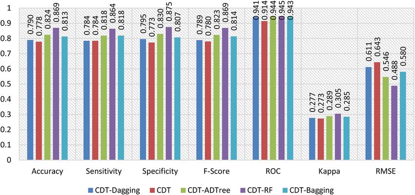
www.nature.com/scientificreports/

                                            Figure 2.  Training performance of the models.

                                            Figure 3.  Validation performance of the models.

                                                The AUROC curve value of CDT-DA, CDT, CDT-ADTree, CDT-RF, and CDT-BA models using calibration
                                            dataset are 0.908, 0.904, 0.938, 0.942, and 0.920 (Figs. 2 and 4a) whereas the values are 0.941, 0.914, 0.944, 0.945,
                                            and 0.943 using training dataset, respectively (Figs. 3 and 4b).
                                                Based on calibration dataset, the accuracy of CDT-DA, CDT, CDT-ADTree, CDT-RF, and CDT-BA models
                                            are 0.778, 0.773, 0.793, 0.812, and 0.788 (Fig. 2) and using validation dataset the accuracy is 0.790, 0.778, 0.824,
                                            0.869, and 0.813, respectively (Fig. 3). The sensitivity of CDT-DA, CDT, CDT-ADTree, CDT-RF, and CDT-BA
                                            models using calibration dataset are 0.776, 0.776, 0.790, 0.810, and 0.790 and specificity is 0.780, 0.771, 0.795,
                                            0.815, and 0.785, respectively (Fig. 2). On the other hand, the sensitivity of CDT-DA, CDT, CDT-ADTree,
                                            CDT-RF, and CDT-BA models using testing dataset are 0.784, 0.784, 0.818, 0.864, and 0.818 and specificity is
                                            0.795, 0.773, 0.830, 0.875, and 0.807, respectively (Fig. 3). Using calibration dataset, F-score of CDT-DA, CDT,
                                            CDT-ADTree, CDT-RF, and CDT-BA models are 0.778, 0.774, 0.792, 0.812, and 0.788 (Fig. 2) whereas using
                                            testing dataset, the F-score values were 0.789, 0.780, 0.823, 0.869, and 0.814, respectively (Fig. 3). The values of
                                            Cohen’s Kappa for CDT-DA, CDT, CDT-ADTree, CDT-RF, and CDT-BA models are 0.637, 0.633, 0.649, 0.665,
                                            and 0.645 using training dataset (Fig. 2 and with testing dataset, the values are 0.277, 0.273, 0.289, 0.305, and
                                            0.285 (Fig. 3), respectively.

          Scientific Reports |   (2021) 11:3147 |                https://doi.org/10.1038/s41598-021-82527-3                                                    6

Vol:.(1234567890)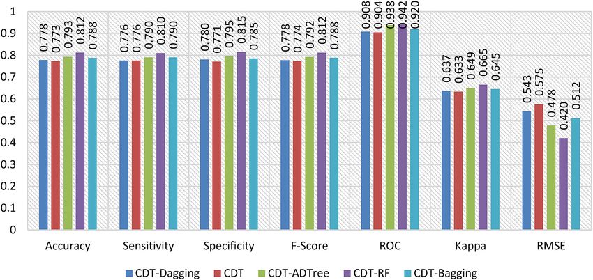
www.nature.com/scientificreports/
Figure 4. Area under the curve of the models in the training and validation data.
Figure 5. Odd ratio values of the models in the training and validation phases.
While using calibration dataset, the RMSE of CDT-DA, CDT, CDT-ADTree, CDT-RF, and CDT-BA models
are 0.543, 0.575, 0.478, 0.420, and 0.512 (Fig. 2) and with testing dataset, the values are 0.611, 0.643, 0.546, 0.488,
and 0.580, respectively (Fig. 3). The odd ratio values of the CDT-DA, CDT, CDT-ADTree, CDT-RF, and CDT-BA
models in training phase are 14.12, 12.35, 21.90, 44.33, and 18.79 whereas in testing phase the values of odd ratio
are 12.29, 11.62, 14.62, 18.71, and 13.79, respectively (Fig. 5). The outcome of validation techniques including
accuracy, sensitivity, specificity, F-score, AUROC, Cohen’s Kappa, odd ratio and RMSE displayed the excellent
predictive ability of models in mapping GES. Based on the training and testing performance of the models, it is
found that CDT-RF was the best model followed by CDT-ADTree, CDT-BA, CDT-DA and CDT models.
The values of SCAI (Fig. 6) generated from GES of CDT-DA, CDT, CDT-ADTree, CDT-RF, and CDT-BA
models increased from very high to very low susceptibility. This outcome of SCAI reveals the enhanced predic-
tive performance of the GES models employed in this study.
Discussion
In recent years, various machine learning33–36, Fuzzy37–41, deep learning42–47, and multiple criteria decision mak-
ing (MCDM) m odels47,48 along with remote s ensing49–53 and geographic information system (GIS)54–56 have been
developed with application in various scientific fields.
Even though the newly developed approaches have advanced from traditional statistical techniques to the
MLAs57–60, recent studies attempt to formulate novel/hybrid models that could achieve better predictive per-
formance than previously employed approaches. Thus, several studies have successfully enhanced the forecast
ability of the MLAs by employing diverse novel ensemble methods. In this study, study we presented a novel
hybrid ensemble for GESM in Bastam sedimentary plain of Northern Iran. We employed five MLAs for model-
ling GES among which four were novel hybrid ensemble models constructed by combining BA, DA, ADTree
Scientific Reports | (2021) 11:3147 | https://doi.org/10.1038/s41598-021-82527-3 7
Vol.:(0123456789)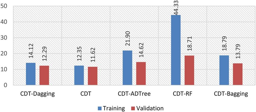
www.nature.com/scientificreports/
Figure 6. Values of seed cell area index (SCAI) in the susceptibility classes.
and RF meta-classifiers with the CDT base classifier and another was an individual CDT. To our knowledge,
the hybrid ensembles used in this research to model GES have been not implemented in any other GESM study.
Fourteen GECFs including clay content, bulk density, elevation, distance to road, distance to stream, drainage
density, lithology, LU/LC, normalized difference vegetation index (NDVI), rainfall, terrain rugged index (TRI),
slit content, slope degree and topography wetness index (TWI) were chosen for the modelling of GES. The
dependency test among the GECFs was carried out which exposed that there was no correlation, thus making
it applicable for processing the outcome.
The importance of GECFs in modelling GES was assessed using the random forest algorithm, which revealed
that drainage density, distance to road, rainfall and NDVI were the most influential factors of GES whereas slope
degree, elevation, silt content, bulk density, TWI and TRI exhibited moderate control over the GES. Similarly,
Pourghasemi et al.8 showed that drainage density, distance to stream, soil content and altitude largely influence
the initiation of GE. Likewise, Arabameri et al.61 determined distance to stream and distance to road to influence
the GES most. Capra et al. (2009)62 reported that formation of GE is higher when the vegetation cover decreases,
and soil wetness increases due to high rainfall. Kariminejad et al.63 determined that silt content and slope angle
influence GES. Arabameri et al.11 showed that topographic factors such as TWI, TRI and elevation has moderate
control over the instigation of GE.
The process-response of a river catchment area is highly influenced by several environmental factors, among
which drainage is the most vital one, which has a strong positive correlation with gully head cut retreat11. The
pattern of drainage is also critical in the initiation and further development of gullies. The drainage pattern in
a river catchment area is highly affected by nature and structure of the geological formation, soil characteris-
egree22. Previous studies on gully erosion have
tics, density of vegetation coverage, infiltration rate, and slope d
shown that initiation and development of gullies are connected to the stream networks and gullying by streams
are responsible where favorable conditions are available for their d evelopment20. The slope instability of an area
is causes by initiation of river and the associated toe erosion and fluctuations of groundwater level. Moreover,
the degree of surface incision is highly dependent on the pattern of drainage network of an area. The develop-
ment and pattern of drainage of an area is directly related to the power of degree of surface i ncision22. The road
and undercutting construction work gradually increases the strain and stress of the slope which significantly
influences slope disturbances and failure20. The pattern and rate of surface runoff is mainly determined through
road networks, and the concentrated surface runoff flow from one catchment area to another leads to steady
increase in watershed size which is ultimately responsible for the process of g ullying20. The major finding of this
research is that CDT-RF (AUSRC = 0.942, AUPRC = 0.945, accuracy = 0.869, specificity = 0.875, sensitivity = 0.864,
RMSE = 0.488, F-score = 0.869 and Cohen’s Kappa = 0.305) was determined to be the finest model having superior
accuracy than the rest of the hybrid models. The CDT-RF is followed by CDT-ADTree, CDT-BA, CDT-DA and
CDT. This clearly shows that RF meta-classifier enhances the predictive performance of individual CDT model.
It is also true in the case of other meta-classifiers, namely ADTree, BA and DA, which improves the forecast
accuracy of the base classifier. The higher performance of RF can be due to utilization of the feature abstraction
method to augment the learning groups for calibrating the base classifiers.
The low predictive accuracy of CDT can be owing to the subset in that the sub-dataset formed is dissimilar
from a particular issue field which generates fairly diverse t rees64. It should also be noted that RF is a powerful
MLA that is derived from random forest algorithm. He et al.65 also showed that RF increases the predictive ability
CDT than any other meta-classifiers such as BA and multiBoostAB (ABM). Nguyen et al.66 also determined that
different meta-classifiers ABM and radial basis function network (RBFN) increases the forecast ability of CDT.
Similarly, both Pham et al.67 and Nguyen et al.68 demonstrated that meta-classifier helps base classifier CDT in
improving the predictive performance in modelling landslide and flash flood vulnerability. From the present
study, it is evident that combining meta-classifier such as RF, ADTree, BA and DA with the base-classifier such
as CDT would increase its performance in accurately predicting GES. The general advantage of meta-classifiers
Scientific Reports | (2021) 11:3147 | https://doi.org/10.1038/s41598-021-82527-3 8
Vol:.(1234567890)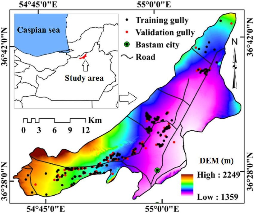
www.nature.com/scientificreports/
Figure 7. Location of study area in Iran. The map was generated using ArcGIS 10.5 software (https://deskt
op.arcgis.com/en/).
is that it enhances the predictive accuracy of the MLAs, whereas individual CDF performs well even in noisy
datasets. The benefit of utilizing BA is that it is most suitable for classifiers with dipping learning curve and it
improves the classification accuracy through the creation of different classifications together. The DA also has
the capability in reducing the noise. The reason for lower performance of individual CDT may be attributed
to the generation of varying trees, which could be owing to the difference in the sub-dataset constructed for a
provided issue domain. The integration of RF with CDT could help the base classifier in decreasing the noise
and bias which would eventually result in the higher accuracy of the ensemble. However, there are certain limita-
tions in these models such as use of various predictor variables with diverse values which need to be addressed
in future studies.
Concluding remarks
Identifying precise and robust algorithms for decreasing inaccuracies in GESM and demarcating GES zones is
crucial. This research employed four novel hybrid ensemble models (CDT-RF, CDT-ADTree, CDT-BA and CDT-
DA) for predicting GES with the aid of fourteen GECFs and 293 gully locations. Various validation measures
including SRC, PRC, specificity, sensitivity, Cohen’s Kappa, F-score, accuracy, RMSE and odd ratio were employed
for assessing the model outcome using both calibration as well as testing dataset. The outcome of cross-checking
revealed that all the employed models had excellent predictive accuracy, among which CDT-RF is identified to
be the most robust model. In addition, the outcome of SCAI also suggests the better performance of the models
in predicting GES. Our study reveals that meta-classifiers increase the predictive efficacy of base classifiers in
modelling GES. The models used in this research can be also applied in other study areas. The GESM generated
by CDT-RF model for Bastam sedimentary plain of Northern Iran can therefore be utilized in controlling the
occurrence of future gullies and sustainable management of soil resources.
Methods
Description of the study area. The Bastam sedimentary plain is one of the most GE prone watersheds
located in the Semnan Province of Northern Iran (Fig. 7). It extends between 36° 25′ 53″ N–36° 45′ 43″ N
latitudes and 54° 43′ 34″ E–55° 10′ 58″ E longitudes and spreads over an area of about 505.06 k m2. The average
elevation of Bastam sedimentary plain is 1577 m.a.s.l (meters above sea level) where the high and low eleva-
tion ranges between 1357 and 2249 m.a.s.l. The high, low and average slope of the study area are 57.96°, 0° and
2.71°, respectively. The annual average precipitation and temperature of this sedimentary plain is 249.5 mm and
14.3 °C, respectively with an arid climate69. Different types of land use/land cover (LU/LC) such as rangeland,
agriculture, forest, woodland, rock and urban occur in the study area that covers nearly 53%, 44.06%, 2%, 0.49%,
0.66%, 0.185% and 0.72%, respectively of the total area in Bastam sedimentary plain. Rangeland is the dominant
vegetation in the study area. The Qal comprising of stream channel, braided channel and flood plain deposits
accounts for more than 90% of study area’s lithology70 (Table 5). The area is characterized by rock outcrops/
entisols, entisols/inceptisols, inceptisols, aridisols and mollisols, covering about 14.77%, 57.11%, 1.61%, 26.33%
and 0.14% of the area, respectively71,72. Among the several soil types found in the present study area, aridisols
cover the maximum portion, constituting the dominant soil type. The evaluation of gullies has indicated that
this area is highly susceptible to gully erosion as nearly 10.34% of the study area is affected by ephemeral gully
erosion. The low slope area is found to be highly susceptible for gully erosion, with the south-central part more
prone to gully erosion as this region is dominated by low slope zone. On the other side, steep slope zone with
rocky outcrops in the northern portion of the study area is conquered by a small number of gullies. Morphomet-
ric analysis of gullies indicates that the length of gullies ranges from few meters to several hundred meters. The
Scientific Reports | (2021) 11:3147 | https://doi.org/10.1038/s41598-021-82527-3 9
Vol.:(0123456789)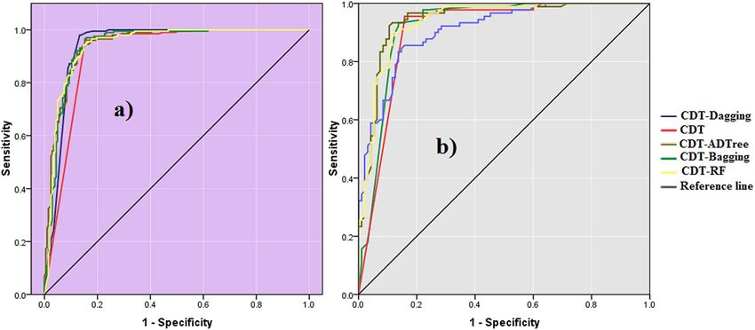
www.nature.com/scientificreports/
Unit Description Area (km2) Area (%)
Yellowish, thin to thick—bedded, fossiliferous argillaceous limestone, dark grey limestone, greenish
DCkh 0.37 0.07
marl and shale, locally including gypsum
Ea.bvs Andesitic to basaltic volcanosediment 8.94 1.77
Ea.bv Andesitic and basaltic volcanics 0.03 0.01
K2m, l Marl, shale and impure limestone 19.67 3.89
Mc Red conglomerate and sandstone 1.51 0.30
Osh Greenish—grey siltstone and shale with intercalations of flaggy limestone 18.09 3.58
P Undifferentiated Permian rocks 454.91 90.07
Qal Stream channel, braided channel and flood plain deposits 1.55 0.31
TRe2 Thick bedded dolomite 0.37 0.07
Table 5. Lithology of study area.
Figure 8. Flowchart of the methodology adopted in the current study.
width also varies from few centimeters to several meters and depths can be as much as several meters. The length
of the gullies ranges from 364 m (maximum) to 0.95 m (minimum) and depths vary from 6.3 to 0.63 m. Our field
survey also reveals that northern part of the study area is dominated by V-shaped cross-section of gullies as this
area is characterized by rocky outcrops and steep slope. However, the central and southern parts are dominated
by U-shaped gullies, as this area is low slope zone with coverage of more erodible soils and more concentrated
runoff and associated erosional activities.
Methodology
The mapping of GES with the help of novel ensemble models, including CDT-BA, CDT-DA, CDT-RF and CDT-
NBT was executed based on the four following phases (Fig. 8). (1) Initially, the spatial distribution of existing
gullies (dependent variable) and GECFs (predictor variables) were prepared for GESM. (2) This was followed by
the assessment of multi-collinearity among GECFs. This evaluation is implemented to eliminate noisy GECFs
and to confirm that there is no correlation among the predictor variables that could affect the prediction of GE.
(3) With the aid of calibration dataset, GESM is generated based on the five models (CDT, CDT-BA, CDT-DA,
CDT-RF and CDT-ADTree). The generation of GESMs is followed by the assessment of each independent factor’s
influence in predicting the GES using random forest model. 4) Using testing dataset, various validation measures
Scientific Reports | (2021) 11:3147 | https://doi.org/10.1038/s41598-021-82527-3 10
Vol:.(1234567890)www.nature.com/scientificreports/
Figure 9. Representative field photographs of the mapped gullies in the study area. (a) Lat: 4072920.7; Long
869988.1 (b) Lat: 4045271.7; Long 846437.7.
such as the area under receiver operating characteristic curve (AUROC), accuracy, sensitivity, specificity, root
mean square error (RMSE), F-score, odd ratio, Cohen Kappa and seed cell area index (SCAI) were applied for
cross-checking the predictive ability of the GESM.
Preparation of gully inventory map. Mapping the extent in the location of gullies in the study area is
indispensable for predicting the GES13. This is because the susceptibility to most of the natural hazards, includ-
ing GE is spatially modelled based on the presumption that gullies that occur in future may follow the identical
conditions that triggered the existing ones61. Thus, understanding the association between the conditioning
factors and previously existing gullies are essential61. We carried out detailed field investigations using the global
positioning system for the preparation of gully inventory map (Fig. 9). A total of 293 gullies were identified in
the Bastam sedimentary plain. These were arbitrarily split into 70% (206 gullies) and 30% (87 gullies) for model
calibration and testing the predictive ability of the m odel13. In addition, an identical number of non-gully loca-
tions were also identified for the processes of model training and validation.
Preparation of gully erosion conditioning factors. GE is an intricate process which is controlled by
numerous factors13,61 although there are no universally accepted factors that are crucial for GESM17. Hence, we
carefully selected 14 GECFs from literature review (Fig. 10) namely (a) elevation, (b) slope, (c)TWI, (d)TRI,
(e) distance to stream, (f) drainage density, (g) distance to road, (h) content of clay, (i) content of silt, (j) bulk
density, (k) NDVI, (l) rainfall, (m) lithology, (n) LU/LC. The GECFs utilized in this research are selected based
on the previous investigations, local geo-environmental circumstances and availability of data11,61,63. All the 14
GECFs employed in this study were created using ArcGIS 10.5. The primary and secondary topographic factors
including elevation, slope degree, TWI and TRI were acquired from ALOS DEM having a spatial resolution
of 12.5 m. The stream network and roads were derived from topographical map with a scale of 1:50,000. The
30 years of rainfall data from 9 stations were utilized for the interpolation of rainfall map using Inverse Distance
Weighting63. Inverse spatial mapping of soil was performed for the areas occupied by gully headcut (GH) mor-
phology. Around 395 soil samples were obtained from the inlets and outlets of GH by digging profile pits rang-
ing between 0 and 2 m in size. While conducting the field investigation, 2 kg of each sample was collected and
transported to the lab, where these were air-dried, followed by soil particle size analyses based on the hydrometer
technique71,72, without eliminating the carbonates, organic matter, and secondary oxides. Secondly, the core
approach73 was utilized for estimating the bulk density. Following this, the techniques proposed by Walkley and
Black (1934)74 and Van B avel75 were employed in measuring the organic matter content and stability of the soil.
Ultimately, the prepared soil layers were added individually to ArcGIS 10.5 and were processed to the scale of
12.5 m × 12.5 m for additional examination. The foremost soil properties, i.e., bulk density, percentages of silt,
and clay content were estimated employing approved petrological techniques and mapped in the GIS.
The lithological units were extracted from maps generated by 1:100,000 (Table 5). The LU/LC of the study area
is acquired from Landsat-8 data. Elevation is considered to be a significant factor that influences the occurrence
of gullies13. It controls the processes of GE owing to its association with various factors such as precipitation, soil
texture, run-off, vegetation type and c over13. The elevation of Bastam sedimentary plain ranges between 1359
and 2249 m. As slope angle influences runoff and drainage density, it is one of the many important factors that
govern gully f ormation24. The slope angle varies from 0 to 57.96%. The TWI is generally applied for assessing
the impact of topography on the infusion of water into the saturated zones of runoff g eneration24. TWI is also an
effective factor that is essential for GESM owing to its association with soil e rosion11, and is computed as f ollows24:
Ds
TWI = ln (1)
tan µ
where Ds and μ denote the upslope contributing region and slope incline, respectively. It also aids in assess-
ing the water content present in the soil owing to upstream catchment area and slope24. TWI of the Bastam
Scientific Reports | (2021) 11:3147 | https://doi.org/10.1038/s41598-021-82527-3 11
Vol.:(0123456789)www.nature.com/scientificreports/
Figure 10. Gully erosion conditioning factors. (a) Elevation, (b) slope, (c) topography wetness index, (d)
terrain rugged index (TRI), (e) distance to stream, (f) drainage density, (g) distance to road, (h) content of clay,
(i) content of silt, (j) bulk density, (k) normalized difference vegetation index (NDVI), (l) rainfall, (m) lithology,
(n) land use/land cover (LU/LC). The map was generated using ArcGIS 10.5 software (https://desktop.arcgi
s.com/en/).
Scientific Reports | (2021) 11:3147 | https://doi.org/10.1038/s41598-021-82527-3 12
Vol:.(1234567890)www.nature.com/scientificreports/
sedimentary plain ranges from 1.728 to 21.04. TRI reflects the terrain morphology and has a considerable effect
on surface runoff24. TRI values range between 0 and 35.45. Since gully initiation is closely associated with stream
networks61, the distance to stream plays a major role in gully formation. The maximum and minimum distance
to stream was 1050 and 0 m. Drainage density is another important factor to be considered while modelling
GES as most of the previous studies have revealed that drainage density is the most influential factor in gully
formation8. The drainage density of the Bastam sedimentary plain ranges from 0.37 and 3.63 km/km2. Building
of roads increases the rigidity of gradients, which also leads to gully formation11. The minimum and maximum
distance to roads are 0 and 9021.57 m. C ouper76 showed that increase in the content of silt and content of clay
would lead to vertical incising of soil, which eventually results in the formation of gullies. The content of clay
varies between 32 and 14%, whereas content of silt ranges from 12 to 43%. The increase in the bulk density of
soil decreases the potential of plants to reduce the soil erosion. The maximum and minimum bulk density ranges
between 1622 and 1491 g cm−3. The rainfall is also a significant factor that controls surface flow and e rosivity11.
The high and low rainfall ranges between 381.12 and 159.20 mm. Vegetation cover has an inverse association
with soil e rosion8. In this study, the red band (b4) and infra-red band (b5) from Landsat 8 data were used for
the computation of NDVI as f ollows8:
NDVI = (b5 − b4)/(b5 + b4) (2)
The value of NDVI ranges from -1 to 1, where values < 0.2 indicates non-vegetation and > 0.2 denotes vegeta-
tion presence. The NDVI of the study area ranges between 0.15 and − 0.55. The wearing down of bare lithological
E17. Table 1 and Fig. 10m provide information of the lithological units existing in the
structures also impacts G
Bastam sedimentary plain. LU/LC is also an important factor considered for G ESM5. Six types of LU/LC are
witnessed in the Bastam sedimentary plain.
Evaluation of multi‑collinearity. It is vital to assess the dependency among the GSCFs before employing
these for GESM as the presence of any correlation would impact the consistency and understanding of model
outcome11. There are numerous techniques including Pearson correlation, variance inflation factors (VIF), ridge
regression, the least absolute shrinkage and selection operator (LASSO), conditional index, elastic net, tolerance
(tol), and jack-knife tests using which multi-collinearity is evaluated. However, commonly, all multi-collinearity
evaluation technique would estimate the dependence between the predictor f actors63. In this study, we adopted
VIF and tol approach for assessing the linear dependency among the GECFs. The expressions of VIF and tol are
as follows:
tol = 1 − ri2 (3)
1
VIF = (4)
tol
where ri2 is attained by reversing all remaining variables in a multivariate r egression11. Since there has been no
approved values of VIF and tol for denoting the collinearity among predictor variables, commonly established
values: tol ≤ 0.1 and VIF ≥ 5 indicates that there is dependency among the independent variables11.
Credal decision tree (CDT). Abellan and Moral (2003)77 introduced CDT for n classification issues
through the application of credal sets78. It utilizes a unique partitioning condition which was created with the
help of uncertainty computation along with inexact p ossibilities78. To circumvent the intricate decision tree
(DT) generation while constructing CDT, an innovative idea was developed, which administered to suspend the
categorization process from growing the cumulative uncertainty owing to the consequence of DT branching78.
A modernized approach was developed with the help of the Dempster and Shafe theory, which is utilized for the
quantification of overall uncertainty from credal sets79. The aforementioned approach is expressed as follows:
CU(n) = NC(n) + RC(n) (5)
where, n denotes a credal set; CU signifies the complete uncertainty value; and NC and RC are functions that
refers to the common non-specificity and common randomness, respectively. The creators of CDT obtained
series of outcomes and successes compared to CU measurement, and furthermore, the computation method of
CU and its attributes are explained orderly in related sources79. The inexact possibility method78 was selected to
investigate the possibility of interims of discrete v ariables79. Assuming ‘W’ as a variable whose values are denoted
with the help of wj, and the identical possibility order p(wj) meets the following e xpression79:
mwj mwj + h
p(wj ) ∈ , (6)
M+h M+h
where, mwj refers to the total number of incidence (W = wj); M represents the sample size and h denotes the
hyperparameter (value: 1 or 2)79.
Bagging (BA). The BA, also popularly known as bootstrap aggregating, enhances the predictive capabilities
of MLAs80. Recent studies show that BA has been successfully employed for precise forecasting of susceptibil-
azards80. Even a minute variation in the calibration data could create a great difference
ity to various natural h
in the model outcome80. BA involves the following stages: (a) arbitrary and independently choosing data from
calibration dataset; (b) formation of several classifier models (CMs) with the help of subgroup datasets and (c)
Scientific Reports | (2021) 11:3147 | https://doi.org/10.1038/s41598-021-82527-3 13
Vol.:(0123456789)www.nature.com/scientificreports/
model generation through the accumulation of every single C Ms81. Integrating the rule of base classifiers has
been confirmed to have a distinguished impact on BA predicting c apability81.
Assume C (ai, bi) as a subset of calibration data which is arbitrarily chosen repetitively from a Calibration
dataset (ai, bi), where ai represents gully presence and bi refers to gully absence. Multiple CMs are generated
based on all subset where Vi(a) represents the created CM. Then finally, every individual classifier (Fi) is com-
bined to form the model outcome (F′). The final prediction of F′ is performed based on the following expression81.
t
F ′ (a) = arg max F(Vi (a) = b) (7)
b∈B i=1
Dagging (DA). The DA is widely used as an ensemble method that is frequently employed for the creation
of meta-classifiers82. There are numerous variations between DA and other techniques such as boosting and BA,
where boosting flexibly alters the calibration dataset according to distribution while the BA adjust the calibration
dataset speculatively and raises bases according to the efficiency of all classifiers as a weight for choosing82. In
DA, the prediction of a model is carried out based on the top vote82. The algorithm utilizes the maximum vote
concept for integrating several classifiers in order to enhance the forecast preciseness of the base classifier. DA
erformance82.
can be employed in case of base classifiers that are a worst case in timely p
Rotation forest (RF). The RF is an established integration method which aids weak classifiers in perform-
ing better1,31. It was introduced by Rodríguez et al.83. It is employed in advancing the variation and precision of
base classifiers according to the feature transformation83. Random forest algorithm serves as the base for the
development of RF, still, RF has the improved capability in handling both multi-dimensional and small dataset83.
The classification possibility of RF algorithm is assessed with the help of the following e xpressions83:
l
vα (a) = fm,n (aSjb )(j = 1, . . . , d) (8)
j=1
a = arg max(vα (a))(v ∈ D) (9)
where, a refers to a classification sample; D represents common groups; l indicates the overall quantity of base
classifiers and Sjb specifies the rotation matrix.
Alternative decision tree (ADTree). ADTree was proposed by Freund and Mason (1999) and is by far
the highly effective decision tree model which is rooted upon the principle of boosting and is widely applied for
modelling purposes19. ADT was hardly employed for GESM in previous studies. It provides good accuracy and
consistency for categorization and forecast issues19. ADTree comprises of two nodes, namely forecast nodes and
judgement nodes19. The components of a calibration dataset are partitioned into forecast nodes through separa-
tion tests, and the equivalent extrapolative values of forecast nodes are acquired. Moreover, through the repeti-
tive estimation, producing and clipping, the ADTree meta-classifier is created that has the affirmative capability
ode19:
to handle intricate and large datasets. The following expression defines the partition testing of forecast n
(10)
T(b) = 2( V+ (b)V− (b) + V+ (−b)V− (−b)) + V ′
where, V + (b) and V − (b) refers to the complete weight of the calibration data which fulfils the circumstance of
c; V′ denotes the overall weight of the dataset which does not fit for the forecast node, and c represents partition
testing. The optimal partition testing is attained by determining the least value of T. The appropriate repetitive
split test is assessed based on a top to bottom approach in ADTree, and the pruning method applied in this
approach is given as follows19:
Tpure = 2( V+ + V− ) + V ′
(11)
where, Tpure refers to the lowest threshold of T that is employed for pruning the estimation of few forecast nodes.
Relative importance assessment of GECFs using random forest. Random forest is a popular non-
parametric MLA which comprises a horde of classification and regression t rees61. Several studies have employed
random forest for the evaluation of the significance of predictive variables84. RF competently handles vague-
ness and unknown data and has the exceptional operational ability even with massive and extremely complex
datasets84. RF comprises two major internal stages. Firstly, it builds several bootstrap samples that are considered
to be calibration sets and then constructs classification rules for every tree. In this process, a few datasets that
were not employed are leftover; these are known as out-of-bag trials (OOB). OOBs are used to evaluate the inac-
curacies in the categorization and to approximate the precision of the p rediction61.
Validation measures. Evaluation of the prediction exactness of a model is essential for concluding the
technical importance of an investigation85. In this study, both training and testing data of GIM is utilized for the
cross-checking of the model outcome1,39. There are two types of validation metrics, i.e. cut-off-independent and
dependent86. The computation of validation metrics stated above is executed with the help of contingency table
Scientific Reports | (2021) 11:3147 | https://doi.org/10.1038/s41598-021-82527-3 14
Vol:.(1234567890)www.nature.com/scientificreports/
which comprises of four components namely TP (true positive), TN (true negative), FN (false negative), and FP
(false positive)87. Apart from these measures, SCAI has also been employed in this study to assess the prediction
accurateness of the calibrated model.
Cut‑off‑independent metrics. The AUROC curve is an extensively utilized metric in various branches
of science for accuracy and efficacy evaluation of predictive model outcomes88,89. It plots the sensitivity on the
Y-axis and 1- specificity on the X-axis90. The value of AUROC varies between 0 and 1, where the value equiva-
lent to unity signifies perfect predictive c apability87. In this research, assessment of success rate curve (SRC) and
prediction rate curve (PRC) were carried out using the calibration and testing data of GIM, where the former is
employed to estimate the learning ability of the algorithm whereas the latter is applied to determine the forecast
capability90. The only difference between PRC and SRC is that testing data is replaced with calibration data in
PRC89.
Cut‑off‑dependent metrics. The measures such as accuracy, sensitivity, specificity, F-score, odd ratio and
Cohen Kappa belongs to the cut-off dependent a pproach89. The sensitivity refers to the possibility of predicting
the gullies precisely as witnessed in actuality, whereas the specificity targets to approximate the likelihood of
predicting non-gullies as perceived in actuality20. The accuracy represents the efficacy of the model as it reveals
the complete success of the forecast model. The F-score is defined as the harmonic average of precision and
recall. The values of F-score varies between 0 and 1 where value near 1 represents high precision and recall. Odd
ratio estimates the chances that an outcome will appear provided a selective display, related to the chances of the
outcome happening in the nonexistence of that display30. Cohen’s Kappa tests the robustness of the model and
aids the modeller to completely comprehend the actual model outcome32. These cut-off-dependent approaches
were utilized for assessing both the training as well as the testing performance of the models used in this study.
The following expressions are employed for the computation of cut-off-dependent m etrics20:
TP
TPR(sensitivity) = (12)
TP + FN
TN
Specificity = (13)
TN + FP
(TN + TP)
accuracy = (14)
(TN + FP + FN + TP)
2TP
F − score = (15)
2TP + FP + FN
TP × TN
odd ratio = (16)
FN × FP
(TP + TN) − [(TP + FN)(TP + FP) + (FN + TN)(FP + TN)]/(T)
Cohen′ s kappa = (17)
(T) − {[(TP + FN)(TP + FP) + (FN + TN)(FP + TN)]/(T)}
Seed cell area index (SCAI). Süzen and Doyuran91 introduced the SCAI method which is known as the
proportion between the total amount of pixels of the particular GES category and the total amount of pixels of
prevailing gullies in that particular GES c ategory86. Numerous studies have employed SCAI for assessing the per-
formance of the forecast models20. The very high value of SCAI for very high susceptibility class and low value of
SCAI for low susceptibility class indicates a perfect model and any contrary outcome of this values denotes the
poor predictive performance of the model.
Statistical measures. The RMSE is employed in this study for the validating the model’s calibration as
well as testing performance. The RMSE of 0.7 and below indicates better predictive ability while a value greater
than 0.7 signifies the poor predictive performance of the model20,32. The RMSE is assessed using the following
expression:
z
RMSE =
1/z (Vp − Va )2 (18)
b=1
where, Vp refers to the value present in calibration or testing data; Va represents the forecast values produced
for the GESMs and z indicates the total number of calibration or testing data.
Received: 12 May 2020; Accepted: 21 January 2021
Scientific Reports | (2021) 11:3147 | https://doi.org/10.1038/s41598-021-82527-3 15
Vol.:(0123456789)www.nature.com/scientificreports/
References
1. Sartori, M. et al. A linkage between the biophysical and the economic: Assessing the global market impacts of soil erosion. Land
Use Policy 86, 299–312 (2019).
2. Poesen, J. Soil erosion in the Anthropocene: Research needs. Earth Surf. Process. Landforms 43, 64–84 (2018).
3. Arabameri, A. et al. A methodological comparison of head-cut based gully erosion susceptibility models: Combined use of statisti-
cal and artificial intelligence. Geomorphology 359, 107136 (2020).
4. Douglas-Mankin, K. R. et al. A comprehensive review of ephemeral gully erosion models. CATENA 195, 104901 (2020).
5. Muhs, D. R. The geochemistry of loess: Asian and North American deposits compared. J. Asian Earth Sci. 155, 81–115 (2018).
6. Kirkby, M. J. & Bracken, L. J. Gully processes and gully dynamics. Earth Surf. Process. Landforms 34, 1841–1851 (2009).
7. Arabameri, A. et al. Spatial modelling of gully erosion using evidential belief function, logistic regression, and a new ensemble of
evidential belief function–logistic regression algorithm. L. Degrad. Dev. 29, 4035–4049 (2018).
8. Pourghasemi, H. R., Sadhasivam, N., Kariminejad, N. & Collins, A. L. Gully erosion spatial modelling: Role of machine learning
algorithms in selection of the best controlling factors and modelling process. Geosci. Front. https: //doi.org/10.1016/j.gsf.2020.03.005
(2020).
9. Poesen, J., Nachtergaele, J., Verstraeten, G. & Valentin, C. Gully erosion and environmental change: Importance and research
needs. in Catena 50, 91–133 (Elsevier, 2003).
10. Rahmati, O., Haghizadeh, A., Pourghasemi, H. R. & Noormohamadi, F. Gully erosion susceptibility mapping: The role of GIS-based
bivariate statistical models and their comparison. Nat. Hazards 82, 1231–1258 (2016).
11. Arabameri, A., Cerda, A. & Tiefenbacher, J. P. Spatial pattern analysis and prediction of gully erosion using novel hybrid model
of entropy-weight of evidence. Water 11, 1129 (2019).
12. Zhao, J., Vanmaercke, M., Chen, L. & Govers, G. Vegetation cover and topography rather than human disturbance control gully
density and sediment production on the Chinese Loess Plateau. Geomorphology 274, 92–105 (2016).
13. Arabameri, A., Chen, W., Lombardo, L., Blaschke, T. & Tien Bui, D. Hybrid computational intelligence models for improvement
gully erosion assessment. Remote Sens. 12, 140 (2020).
14. Arabameri, A. et al. Evaluation of recent advanced soft computing techniques for gully erosion susceptibility mapping: A compara-
tive study. Sensors 20, 335 (2020).
15. Meliho, M., Khattabi, A. & Mhammdi, N. A GIS-based approach for gully erosion susceptibility modelling using bivariate statistics
methods in the Ourika watershed Morocco. Environ. Earth Sci. 77, 1–14 (2018).
16. Conoscenti, C. et al. Gully erosion susceptibility assessment by means of GIS-based logistic regression: A case of Sicily (Italy).
Geomorphology 204, 399–411 (2014).
17. Dube, F. et al. Potential of weight of evidence modelling for gully erosion hazard assessment in Mbire District, Zimbabwe. Phys.
Chem. Earth 67–69, 145–152 (2014).
18. Hosseinalizadeh, M. et al. How can statistical and artificial intelligence approaches predict piping erosion susceptibility?. Sci. Total
Environ. 646, 1554–1566 (2019).
19. Arabameri, A. et al. Comparison of machine learning models for gully erosion susceptibility mapping. Geosci. Front. 11, 1609–1620
(2020).
20. Saha, S., Roy, J., Arabameri, A., Blaschke, T. & Tien Bui, D. Machine learning-based gully erosion susceptibility mapping: A case
study of Eastern India. Sensors 20, 1313 (2020).
21. Amiri, M., Pourghasemi, H. R., Ghanbarian, G. A. & Afzali, S. F. Assessment of the importance of gully erosion effective factors
using Boruta algorithm and its spatial modeling and mapping using three machine learning algorithms. Geoderma 340, 55–69
(2019).
22. Arabameri, A., Pradhan, B., Pourghasemi, H. R., Rezaei, K. & Kerle, N. Spatial modelling of gully erosion using GIS and R pro-
graming: A comparison among three data mining algorithms. Appl. Sci. 8, 1369 (2018).
23. Gayen, A. & Pourghasemi, H. R. Spatial Modeling of Gully Erosion: A New Ensemble of CART and GLM Data-Mining Algorithms.
in Spatial Modeling in GIS and R for Earth and Environmental Sciences 653–669 (Elsevier, 2019). doi:https://doi.org/10.1016/b978-
0-12-815226-3.00030-2
24. Garosi, Y. et al. Comparison of differences in resolution and sources of controlling factors for gully erosion susceptibility mapping.
Geoderma 330, 65–78 (2018).
25. Gutiérrez, Á. G., Schnabel, S. & Lavado Contador, J. F. Using and comparing two nonparametric methods (CART and MARS) to
model the potential distribution of gullies. Ecol. Modell. 220, 3630–3637 (2009).
26. Arabameri, A., Pradhan, B. & Lombardo, L. Comparative assessment using boosted regression trees, binary logistic regression,
frequency ratio and numerical risk factor for gully erosion susceptibility modelling. CATENA 183, 104223 (2019).
27. Cao, B. et al. Hybrid microgrid many-objective sizing optimization with fuzzy decision. IEEE Trans. Fuzzy Syst. 1, 1. https://doi.
org/10.1109/tfuzz.2020.3026140 (2020).
28. Liu, S., Yu, W., Chan, F. T. S. & Niu, B. A variable weight-based hybrid approach for multi-attribute group decision making under
interval-valued intuitionistic fuzzy sets. Int. J. Intell. Syst. https://doi.org/10.1002/int.22329 (2020).
29. Peng, S., Zhang, Z., Liu, E., Liu, W. & Qiao, W. A new hybrid algorithm model for prediction of internal corrosion rate of multiphase
pipeline. J. Nat. Gas Sci. Eng. 1, 103716 (2020).
30. Arabameri, A. et al. Gully head-cut distribution modeling using machine learning methods-a case study of N.W. Iran. Water
(Switzerland) 12, 16 (2020).
31. Chowdhuri, I. et al. Implementation of artificial intelligence based ensemble models for gully erosion susceptibility assessment.
Remote Sens. 12, 3620 (2020).
32. Roy, J. & Saha, S. Integration of artificial intelligence with meta classifiers for the gully erosion susceptibility assessment in Hinglo
river basin Eastern India. Adv. Sp. Res. https://doi.org/10.1016/j.asr.2020.10.013 (2020).
33. Fu, X. & Yang, Y. Modeling and analysis of cascading node-link failures in multi-sink wireless sensor networks. Reliab. Eng. Syst.
Saf. 1, 106815. https://doi.org/10.1016/j.ress.2020.106815 (2020).
34. Qu, S., Han, Y., Wu, Z. & Raza, H. Consensus modeling with asymmetric cost based on data-driven robust optimization. Group
Decis. Negot. https://doi.org/10.1007/s10726-020-09707-w (2020).
35. Tsai, Y.-H. et al. A BIM-based approach for predicting corrosion under insulation. Autom. Constr. 107, 102923. https://doi.
org/10.1016/j.autcon.2019.102923 (2019).
36. Wang, S., Zhang, K., van Beek, L. P. H., Tian, X. & Bogaard, T. A. Physically-based landslide prediction over a large region: Scaling
low-resolution hydrological model results for high-resolution slope stability assessment. Environ. Modell. Softw. 1, 104607. https
://doi.org/10.1016/j.envsoft.2019.104607 (2019).
37. Cao, B. et al. Multiobjective evolution of fuzzy rough neural network via distributed parallelism for stock prediction. IEEE Trans.
Fuzzy Syst. 1, 1. https://doi.org/10.1109/tfuzz.2020.2972207 (2020).
38. Shi, K., Wang, J., Tang, Y. & Zhong, S. Reliable asynchronous sampled-data filtering of T-S fuzzy uncertain delayed neural networks
with stochastic switched topologies. Fuzzy Sets Syst. 381, 1–25. https://doi.org/10.1016/j.fss.2018.11.017 (2020).
39. Shi, K., wang, J., Zhong, S., Tang, Y. & Cheng, J. Non-fragile memory filtering of T-S fuzzy delayed neural networks based on
switched fuzzy sampled-data control. Fuzzy Sets Syst. https://doi.org/10.1016/j.fss.2019.09.00 (2019).
Scientific Reports | (2021) 11:3147 | https://doi.org/10.1038/s41598-021-82527-3 16
Vol:.(1234567890)You can also read