Cross-population coupling of neural activity based on Gaussian process current source densities
←
→
Page content transcription
If your browser does not render page correctly, please read the page content below

Cross-population coupling of neural activity based on
                                                         Gaussian process current source densities
                                                         Natalie Klein1, 2¤ , Joshua H. Siegle3 , Tobias Teichert4 , Robert E. Kass1, 2, 5*

                                                         1 Department of Statistics and Data Science, Carnegie Mellon University, Pittsburgh,
                                                         Pennsylvania, USA
                                                         2 Machine Learning Department, Carnegie Mellon University, Pittsburgh, Pennsylvania,
                                                         USA
                                                         3 MindScope Program, Allen Institute, Seattle, Washington, USA
arXiv:2104.10070v3 [stat.AP] 8 Nov 2021

                                                         4 Departments of Psychiatry and Bioengineering, University of Pittsburgh, Pittsburgh,
                                                         Pennsylvania, USA
                                                         5 Neuroscience Institute, Carnegie Mellon University, Pittsburgh, Pennsylvania, USA
                                                         * kass@stat.cmu.edu
                                                         ¤Current address: Statistical Sciences Group, Los Alamos National Laboratory, Los
                                                         Alamos, New Mexico, USA

                                                         Abstract
                                                         Because local field potentials (LFPs) arise from multiple sources in different spatial
                                                         locations, they do not easily reveal coordinated activity across neural populations on a
                                                         trial-to-trial basis. As we show here, however, once disparate source signals are
                                                         decoupled, their trial-to-trial fluctuations become more accessible, and cross-population
                                                         correlations become more apparent. To decouple sources we introduce a general
                                                         framework for estimation of current source densities (CSDs). In this framework, the set
                                                         of LFPs result from noise being added to the transform of the CSD by a biophysical
                                                         forward model, while the CSD is considered to be the sum of a zero-mean, stationary,
                                                         spatiotemporal Gaussian process, having fast and slow components, and a mean
                                                         function, which is the sum of multiple time-varying functions distributed across space,
                                                         each varying across trials. We derived biophysical forward models relevant to the data
                                                         we analyzed. In simulation studies this approach improved identification of source
                                                         signals compared to existing CSD estimation methods. Using data recorded from
                                                         primate auditory cortex, we analyzed trial-to-trial fluctuations in both steady-state and
                                                         task-evoked signals. We found cortical layer-specific phase coupling between two probes
                                                         and showed that the same analysis applied directly to LFPs did not recover these
                                                         patterns. We also found task-evoked CSDs to be correlated across probes, at specific
                                                         cortical depths. Using data from Neuropixels probes in mouse visual areas, we again
                                                         found evidence for depth-specific phase coupling of primary visual cortex and
                                                         lateromedial area based on the CSDs.

                                                         Author summary
                                                         To better understand information processing in the brain, it is important to identify
                                                         situations in which neural activity is coordinated across populations of neurons,
                                                         including those in distinct layers of the cortex. Bulk population activity results in
                                                         voltage changes across extracellular electrodes, but in raw form such voltage recordings
                                                         can be hard to analyze and interpret. In this paper, we develop a novel framework for
                                                         locating the sources of currents that produce the measured voltages, and decomposing

                                      November 9, 2021                                                                                        1/31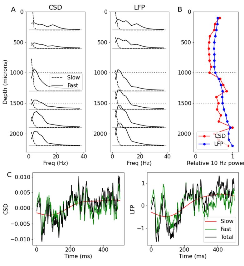
those currents into interpretable components. We use this flexible framework to develop
                   statistical methods of analysis, and we show that our methodology can be more effective
                   than existing techniques for current source localization. We apply the method to
                   extracellular recordings in two contexts: primate auditory cortex in response to tone
                   stimuli, and mouse visual cortex in response to visual stimuli. In both cases, we get
                   results that are useful for understanding cross-population activity while being difficult
                   or impossible to obtain using the raw voltage signals. We thereby demonstrate the
                   broad utility of our approach for identifying coordinated neural activity based on
                   extracellular voltage recordings.

                   Introduction
                   Local field potentials (LFPs) recorded from multiple electrodes are influenced in part by
                   interactions among populations of neurons. However, because they involve a variety of
                   post-synaptic potentials near the recording electrode [1, 2], and may also be affected by
                   more distant sources [3–6], using LFPs to identify cross-population co-activity is
                   difficult: it can be hard to disentangle the many signals mixed together in LFPs, which
                   may have multiple timescales and likely arise from distributed current sources
                   contaminated by noise. We have developed and investigated a statistical modeling
                   approach that incorporates the biophysical relationship between cellular current flow
                   and measured voltages, and assumes the current source densities are stochastic, driven
                   by several distinct processes, each operating at a different timescale. The goal of our
                   work is to identify trial-to-trial covariation among features of the current source
                   densities, using such covariation as an indicator of coordinated activity across neural
                   populations. As we show, relationships across populations can become apparent when
                   analyzing current source densities even though they are invisible among LFPs.
                       Traditional current source density (CSD) estimation is based on a particular forward
                   model, and it applies second derivatives along a discrete grid of locations [7, 8]. This not
                   only restricts its application to LFPs from evenly-spaced recording electrodes, but it
                   also makes traditional CSD estimation sensitive to noise because second derivatives of
                   noisy functions are unstable [9]. Our approach is closer, in spirit, to a pair of more
                   recent suggestions, termed inverse CSD [10] and kernel CSD [11], but includes
                   important additional structure. We apply a forward model while assuming there are
                   both steady (spontaneous) and transient (evoked) currents, with the steady currents
                   having fast and slow components; these currents are then mapped to the voltage
                   detected at each electrode using a forward model, and we assume noise is added to
                   produce the LFP. In schematic form, our modeling approach can be written,
                                            CSD     =    transient + slow + fast
                                            LFP     =    forward(CSD) + noise
                   where the slow and fast terms on the right of the CSD equation are spatiotemporal
                   Gaussian processes with different timescales. From this intuitive conception we have
                   constructed a framework for finding trial-to-trial correlation, across populations, both in
                   transient current increases and in steady but rapidly changing currents (oscillations).
                   This framework, spelled out in Eqs (1)-(4) in the next section, is able to improve
                   identification of currents substantially while also offering flexibility: it can be used to
                   analyze data from electrodes spaced unevenly in 1, 2, or 3 spatial dimensions, and it
                   allows parameter-tuning in conjunction with model fitting. Furthermore, even though
                   the non-evoked activity is assumed to have only two components, the model is able to
                   reproduce the spectra of measured LFPs. Because the framework is built around
                   Gaussian process current source densities, we use the acronym GPCSD to refer to the
                   methodology and resulting CSD estimates.

November 9, 2021                                                                                          2/31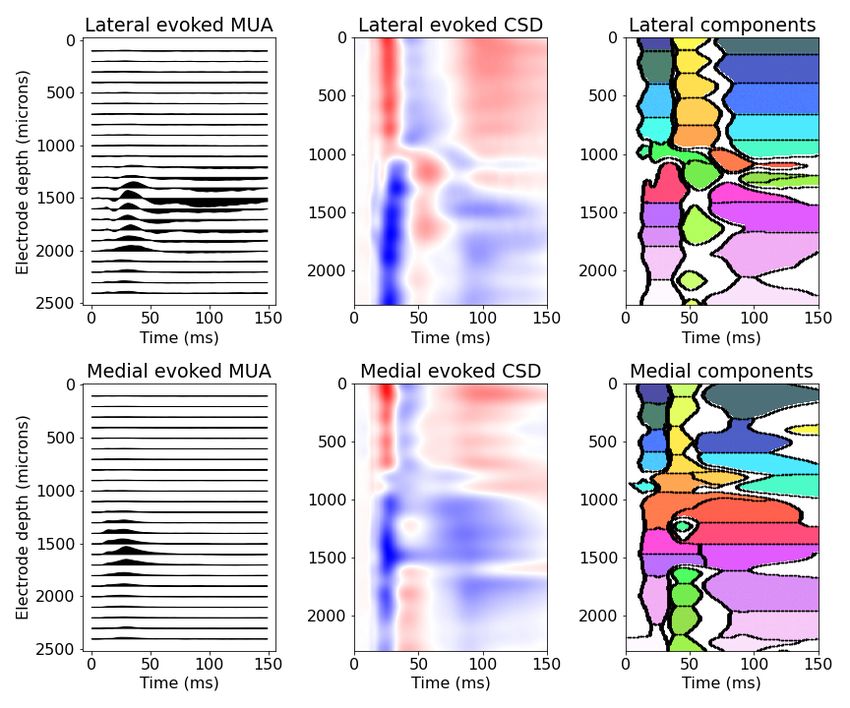
The forward model maps the source space into a lower-dimensional observation
                   space. Estimation of sources from data therefore creates an ill-posed inverse problem.
                   GPCSD effectively regularizes by using a flexible Gaussian process structure with a
                   relatively low-dimensional parameter space. We confirm here, using simulated data,
                   that our approach can outperform existing methods in recovering ground truth CSDs,
                   even when the modeling assumptions are incorrect. We then illustrate potential findings
                   by analyzing two data sets: LFPs from a pair of laminar probes in primate auditory
                   cortex, in response to auditory cues, and LFPs from Neuropixels [12] in distinct visual
                   areas of the mouse, in response to visual stimuli [13]. In the case of the auditory data,
                   we extracted dense spatial profiles of CSD activity operating at different time scales,
                   and identified 10Hz phase coupling across populations at similar cortical depths, and
                   also across different depths; these relationships were not recovered by applying phase
                   coupling methods directly to the recorded LFPs. Previous work suggests that current
                   sources are useful for understanding trial-to-trial variation [14], so we also used CSDs to
                   identify trial-to-trial correlation in evoked responses to an auditory stimulus [15]. Using
                   the LFPs from Neuropixels we found depth-specific phase coupling of primary visual
                   cortex (V1) and lateromedial area (LM) in both theta and beta bands. Together, the
                   simulation and real data results demonstrate the possibility of inferring cooperative
                   population activity from LFPs.
                       In the following sections, we first describe the general statistical formulation of our
                   approach, including details about our forward modeling. This framework is general. To
                   apply it in a given problem, choices must be made. We specify these particulars in the
                   context of both simulated and real data. We then present our data-analytic results.

                   Results
                   Statistical formulation of CSD estimation
                   In this section, we describe our conception of the CSD as a spatiotemporal stochastic
                   process, we outline the general form of the forward model, and we show how we adapt it
                   to our one-dimensional and two-dimensional data applications.

                   CSD as a spatiotemporal process
                   Biophysical forward models describe the transformation from currents to recorded
                   voltages at any instant in time. In this work, we use the term “biophysical forward
                   model” to refer to a simplified forward model based on simplifying assumptions; in
                   particular, we do not include details such as properties of specific neurons in the
                   forward models. Current flow across a cell membrane creates a current source or sink,
                   and the resulting three-dimensional field potential can be derived using volume
                   conductor theory. Because it is not possible to determine all the contributions of
                   individual transmembrane currents from measured LFPs, the CSD at time t and spatial
                   point s may be conceptualized as the average transmembrane current within a small
                   area around s [2]. We let c(s, t) denote the CSD, taking it to be a continuous function,
                   which we will estimate from the LFP data. The biophysical model maps the CSD c to
                   the field potential, which we write as φ, through a spatial linear operator As , so that
                   φ = As [c]. We use the subscript s to emphasize the spatial operation. The operator
                   takes the form of an integral, so that the field potential at (s, t) is given by
                                                                   Z
                                           φ(s, t) = As [c](s, t) = a(s, s0 )c(s0 , t)ds0                 (1)

November 9, 2021                                                                                         3/31
for a suitable function a(s, s0 ) (the form of which will become clear). We write the
                   measured LFP as φ̃ and assume it is equal to φ plus independent noise:

                                                       φ̃(s, t) = φ(s, t) + (s, t).                              (2)

                   Across repeated trials, in response to the same stimulus or producing the same behavior,
                   the CSD will vary [15]. We use a superscript r to identify relevant quantities on trial r,
                   for r = 1, . . . , Nr , and we assume the CSD functions c(r) (s, t) are independent
                   realizations of a stochastic process. Finally, we assume the CSD c(s0 , t) is the sum of
                   three components operating at distinct timescales, an evoked transient mean µ(s0 , t), a
                   slowly varying stationary process η1 (s0 , t), and a more rapidly varying stationary
                   process η2 (s0 , t). This last process η2 could be oscillatory. Thus, on trial r we have
                                                                           (r)           (r)
                                          c(r) (s0 , t) = µ(r) (s0 , t) + η1 (s0 , t) + η2 (s0 , t),              (3)

                   so that c(r) (s0 , t) becomes a realization of a stochastic process, the realizations being
                   independent across trials. Because As is linear, on trial r we get
                                                                     (r)                (r)
                              φ̃(r) (s, t) = As [µ(r) ](s, t) + As [η1 ](s, t) + As [η2 ](s, t) + (r) (s, t).    (4)

                       Eqs (1)-(4), together with estimation of the current source density from the LFP
                   data, define the fundamental components of the framework we have developed. By
                   taking η1 and η2 to be Gaussian processes, the functions c(r) (s0 , t) in Eq (3) become
                   Gaussian process current source densities, and we are able to infer features of them, on
                   a trial-by-trial basis. More specifically, the free parameters in Eq (3), together with a
                   free parameter in our forward model, make up a parameter vector θ for a log likelihood
                   function (see Eq (15)), and the current source density on trial r is estimated using the
                   collection of φ̃(r) (s, t) observations across the relevant grid of (s, t) values (Eq (17)). As
                   we will show, this model can generate multiple time series similar to those observed in
                   LFPs [1]. The specifications of the forward model in Eq (1) and the three terms on the
                   right of Eq (3) are application-dependent. We discuss them below in the context of our
                   two data sets.

                   Forward model details
                   We first give an overview of a commonly-used three-dimensional forward model, which
                   is relevant when three-dimensional LFP recordings are available. In the following
                   section we describe additional a priori physical models that are required to adapt the
                   generative model and forward model to LFP measurements from one-dimensional and
                   two-dimensional electrode arrays.
                       Previous work on CSD estimation has established that an assumption of an isotropic,
                   homogeneous medium with scalar conductivity ς is a reasonable approximation for
                   cortical signals in primates [16]; see also the discussion of forward modeling assumptions
                   in [17, Section 4.2.1]. Using the quasi-static assumption, the relationship between the
                   CSD c and the LFP φ at a single time point (time index suppressed for clarity of
                   notation) is governed by the Poisson equation [7]:
                                              2
                                              ∂ φ(x, y, z) ∂ 2 φ(x, y, z) ∂ 2 φ(x, y, z)

                      ς∇ · (∇φ(x, y, z)) = ς                +               +               = −c(x, y, z), (5)
                                                  ∂x2              ∂y 2            ∂z 2

                   where the spatial location s is described in terms of coordinates (x, y, z). While this
                   appears to give a formula for computing the CSD from the LFP, it requires detailed,
                   accurate knowledge of the LFP in three dimensions, without which it fails to accurately
                   recover the CSD [18]. In addition, estimated second derivatives are highly influenced by

November 9, 2021                                                                                                 4/31
noise. However, assuming an infinite volume conductor with negligible boundary
conditions, the differential equation may be inverted to an integral equation which
instead gives φ in terms of a linear integral operator As on c [8]:
c(x0 , y 0 , z 0 )
Z Z Z
1
φ(x, y, z) = As [c](s) ≡ − p dx0 dy 0 dz 0 .
4πς (x − x0 )2 + (y − y 0 )2 + (z − z 0 )2
(6)
Adapting the model
Though our generative model and forward model have thus far been discussed in terms
of general processes over three dimensions, it is common for electrodes to be arrayed
along only one or two dimensions, which leaves unmeasured the effects in other
dimensions. One advantage of the formulation we have described is that it can be
adapted to these situations by introducing a priori assumptions about the CSD in the
unmeasured directions.
One-dimensional recordings are typically taken along a linear probe inserted
perpendicular to the surface of the cortex, so we will index the one-dimensional spatial
locations by a single coordinate z representing depth along the probe. We use an a
priori physical model in which the CSD is assumed constant in the dimensions
perpendicular to the linear probe on a cylinder of radius R around the probe and zero
elsewhere [10]; previous work has shown deviations from this shape do not have a large
impact on the results [11, 19]. Additionally, as linear probes are typically inserted to
penetrate the thickness of the cortex, we assume the CSD is nonzero only on an interval
a ≤ z ≤ b representing the thickness of the cortex. These assumptions lead to the
following a priori physical model that describes the variation of the CSD in the z
direction through a function g(z, t) that varies over time and a single spatial dimension:
c(x, y, z, t) = g(z, t)1(x2 + y 2 ≤ R)1(a ≤ z ≤ b). (7)
In Eq (7), 1(·) is an indicator function that evaluates to 1 if the argument is true and 0
otherwise, and we have used the convention that x = y = 0 corresponds to the probe
location. Under this a priori physical model, as shown in S1 Text. Modeling and
computational details and additional simulation results and previously derived in [10],
the three-dimensional forward model of Eq (6) reduces to
s s
Z b 0
2 0
2
R z−z z−z
φ(z, t) = Az [g](z, t) ≡ − g(z 0 , t) +1− dz 0 . (8)
2ς a R R
| {z }
a(z,z 0 ;R)
Thus, under this a priori physical model, the one-dimensional LFP is the result of
applying a linear operator Az to g, where the weighting function a(z, z 0 ; R) (see Eq (1))
decreases with distance z − z 0 but also depends on the cylinder radius R. In this case,
our prior model on the CSD specifies the space of functions g(z, t) with one spatial and
one temporal dimension.
Two-dimensional LFP measurements are commonly collected using microelectrode
arrays such as a Utah array or Neuropixels probe [12, 20]. In the Neuropixels data we
will analyze, the two-dimensional spatial locations represent depth and width along the
probe, so we index the spatial location s by coordinates y for width and z for depth.
Unlike with Utah arrays, for Neuropixels, sources behind the face housing the electrode
contacts are unlikely to make contributions to the measured LFPs [21], so we assume
they don’t. We also assume zero charge in a small area in front of the probe face, which
avoids singularities in the forward model. Therefore, the a priori physical model will
November 9, 2021 5/31assume that the CSD is constant in front of the face of the probe in the unmeasured x
direction for some distance R after a space of τ ; that is, using the convention that x = 0
is the face of the probe and positive x are in front of the probe, we assume
c(x, y, z, t) = g(y, z, t)1(τ ≤ x ≤ R + τ )1(az ≤ z ≤ bz )1(ay ≤ y ≤ by ). (9)
We note that this forward model is similar to previously derived models for
multielectrode arrays [22, 23]. In this case, the three-dimensional forward model of
Eq (6) reduces to (see S1 Text. Modeling and computational details and additional
simulation results for derivation)
φ(y, z, t) = Ay,z [g](y, z, t)
q
1
Z bz Z by R+τ + (R + τ )2 + ry2 + rz2
≡− g(y 0 , z 0 , t) log q dy 0 dz 0 .
4πς az ay 2 2 2
τ + τ + ry + rz )
| {z }
a(y,y 0 ,z,z 0 ;R,τ ) where ry =y−y 0 , rz =z−z 0
(10)
The prior in this case specifies the space of functions g(y, z, t) with two spatial
dimensions and one temporal dimension. We note that the form of the forward model is
similar to existing two-dimensional forward models for slightly different measuring
devices such as Utah arrays [11], but with some differences due to the a priori physical
model we have assumed for the Neuropixels probe.
Modeling and implementation details
The framework in Eqs (1)-(4) is very flexible and must be adapted to the particulars of
each situation. In this section, we discuss specific distributional modeling choices for the
two data sets we analyze here. We also provide implementation details for model
estimation and inference. The Python code implementing the methodology presented in
this paper is available at Zenodo [24] and as a Python package on pyPI
https://pypi.org/project/gpcsd/, with full source code at
https://github.com/natalieklein/gpcsd.
CSD prior model
In Eq (4), the noise is modeled as zero-mean Gaussian, independent over space and
time, with variance σ 2 (though extensions to spatially or temporally varying noise
variances are easily included without complicating the computational framework).
Details of the transient mean µ(r) = µ(r) (s0 , t) differ depending on the application, so
specific choices will be discussed in context; in the remainder of this section, we will
assume µ(r) is known and that it absorbs the non-stationary activity. The η processes
are then modeled as independent zero-mean Gaussian processes that are stationary in
time and space, with realizations being independent across trials. To complete the
model specification, we assume the spatiotemporal covariance for the sum of the slow
and fast processes is separable in space and time. That is, the covariance at (s, t) and
(s0 , t0 ) decomposes as
k(s, t; s0 , t0 ) = k s (s, s0 )[k(1)
t
(t, t0 ) + k(2)
t
(t, t0 )]. (11)
Compared with a non-separable covariance structure, separability greatly reduces the
number of free parameters in the model and yields large savings in computation time.
As we show in our simulation and real-data results, it remains possible to fit spatially
November 9, 2021 6/31distinct sources that have different profiles in time. While in principle, processes at
multiple time scales may not be identifiable, we distinguish between the slow and fast
processes using priors on the lengthscale parameters.
One of the advantages of our generative model framework is that various spatial and
temporal covariance functions can be used to include different prior beliefs about the
underlying process, including its smoothness in space and time or periodicity; an
overview of commonly-used covariance functions is given in [25, Ch. 4]. In our
simulations and data analysis, we use the following covariance function structure. The
spatial covariance function is a unit variance squared exponential, or SE, with one
lengthscale for each of the D spatial dimensions:
D
!
0 2
X (sd − s )
k s (s, s0 ) = exp − d
.
2`2s,d
d=1
The SE covariance function reflects the prior belief that the CSD is smooth over space
with the lengthscale `s,d governing the frequency of variation along spatial dimension d.
The slow-timescale temporal covariance function is also SE,
!
t 0 2 (t − t0 )2
k(2) (t, t ) = σ2 exp − ,
2`2t,2
with σ22 representing the marginal variance of the slow-timescale process and `t,2
representing the frequency of variation. The fast-timescale exponential covariance
function can capture rougher, faster variations,
|t − t0 |
t
k(1) (t, t0 ) = σ12 exp − ,
`t,1
and has marginal variance σ12 and lengthscale `t,1 . Note that the spatial covariance
function has unit variance to avoid identifiability issues with the marginal temporal
variances.
Denoting by Ks,t;s0 ,t0 the spatiotemporal covariance matrix of the combined fast and
slow CSD processes evaluated for vectors of spatial and temporal locations s, s0 , t, and
t0 , the covariance matrix has the following structure:
Ks,t;s0 ,t0 = Kss,s0 ⊗ Kt(1)t,t0 + Kt(2)t,t0 .
Exploiting the covariance matrix structure allows faster matrix inversion that would be
possible on a general spatiotemporal covariance matrix [26].
Joint distribution of CSD and LFP
We have now specified the generative model framework for the CSD in addition to
forward models relating the CSD to the LFP for one-, two-, and three-dimensional
recordings. Before discussing how the CSD can be predicted using this model or how to
fit the model, we give an overview of what the generative model and forward model
imply about the joint distribution of the latent CSD and the observed LFPs.
Assuming we are working with LFPs measured in one or two spatial dimensions, our
generative model provides the form of g(s, t) describing the spatial and temporal
variation of the CSD in the measured dimensions. The generative CSD model gives g as
a Gaussian process with mean function µ and covariance function k s [k(1)
t t
+ k(2) ], which
we denote as
g ∼ GP (µ, k s [k(1)
t t
+ k(2) ]).
November 9, 2021 7/31Much as in the finite-dimensional case, the application of a linear operator to a
Gaussian process results in another process that is jointly Gaussian with the original
process. We write the bilinear operator corresponding to As , when applied to k s , as
As [k s ]ATs , so that the marginal noiseless LFP process is given by
φ ∼ GP (As [µ], As [k s ]ATs [k(1)
t t
+ k(2) ]).
See Eq (S.7) in S1 Text. Modeling and computational details and additional simulation
results.
The joint Gaussian process governing the CSD and LFP processes implies that if we
have noisy observations of φ̃ at a discrete set of spatial locations s and temporal
locations t, then the joint distribution of the vectorized observations, denoted φ̃s,t , and
the vectorized CSD process observed at an arbitrary set of locations s0 and t0 , denoted
gs0 ,t0 , is multivariate Gaussian:
s
Ks0 ,s0 ⊗ Ktt0 ,t0 Kss0 ,s ATs ⊗ Ktt0 ,t
gs0 ,t0 µs0 ,t0
∼N , , (12)
φ̃s,t As µs,t As Kss,s0 ⊗ Ktt,t0 As Kss,s ATs ⊗ Ktt,t + σ 2 I
where Ktt0 ,t0 = Kt(1),t0 ,t0 + Kt(2),t0 ,t0 . Note that Eq (12) refers to the joint distribution of
CSD and LFP processes on a single trial, for notational clarity; to complete the model
across trials, we assume the trials are independently and identically distributed. The
linear operator notation As Kss,s ATs indicates application of the linear operator jointly to
both inputs of the covariance function used to compute Ks,s , while As Kss,s0 and
Kss0 ,s ATs indicate application of the linear operator to only the first or second inputs,
respectively. Details of these calculations are given in S1 Text. Modeling and
computational details and additional simulation results. The joint distribution over
discretely observed LFPs and the latent CSD process at any spatial and temporal
coordinates of interest is used for tuning model parameters and for prediction of the
CSD.
Estimation of model parameters
Using properties of multivariate Gaussian distributions, Eq (12) implies that the
marginal density of the observations for trial r, defined as
(r) Z (r)
p φ̃s,t = p φ̃s,t |gs0 ,t0 p(gs0 ,t0 ) dgs0 ,t0 , (13)
is available in closed form:
(r)
φ̃s,t ∼ N (As µs,t , As Kss ATs ⊗ Ktt + σ 2 I). (14)
Taking all Nr trials to be independent and identically distributed, we obtain the
following
h log marginal likelihood function i for the model parameters
D
θ = R, {`s,d }d=1 , `t,1 , `t,2 , σ12 , σ22 , σ 2 :
N
r
Nr 1X (r) T (r)
log L(θ) = − log (|Σ|) − φ̃s,t Σ−1 φ̃s,t , (15)
2 2 r=1
where Σ ≡ Kss,s ⊗ Ktt,t + σ 2 I depends implicitly on the covariance hyperparameters
D
[{`s,d }d=1 , `t,1 , `t,2 , σ12 , σ22 ] and on the forward model hyperparameter R. Note that
direct inversion of Σ is costly and potentially unstable, but can be improved by
exploiting the Kronecker product structure (S1 Text. Modeling and computational
details and additional simulation results).
November 9, 2021 8/31To estimate the model parameters, we use the log marginal posterior, which
combines the log marginal likelihood with prior information about the model
parameters:
p(θ|φ̃s ) ∝ p(φ̃s )p(θ). (16)
While a fully Bayesian approach such as MCMC could be used to approximate the full
posterior, we instead use maximum a posteriori (MAP) estimation by maximizing the
logarithm of Eq (16) with respect to θ; in this case, the use of priors can be seen as a
form of regularization on the log marginal likelihood that discourages unrealistic or
unidentifiable parameter values. In our implementation, we use inverse Gamma priors
for the lengthscales in which the prior hyperparameters are chosen so that the 1% and
99% quantiles will fall at specific values, typically corresponding to the minimum and
maximum observed distances in space or time [27]. We also use a similar inverse
Gamma prior for the forward model parameter R, and use broad half-Normal priors for
the marginal variances and the noise variance [27].
Predicting the CSD
Given a fixed mean function and fixed values for model parameters for the covariance
functions and forward model, predictions conditional on the observed values of φ̃ can be
made for any s0 , t0 for either φ or g; typically, we will be mostly interested in predicting
the latent CSD described by g. Using properties of multivariate Gaussians, Eq (12)
yields the following distribution for the CSD conditioned on the observed LFPs:
gs0 ,t0 φ̃s,t ∼ N (µ∗ , K∗ ) .
The conditional mean, which we use to predict gs0 ,t0 given φ̃s,t , is
µ∗ = µs0 ,t0 + As Kss0 ,s ⊗ Ktt0 ,t [As Kss,s ATs ⊗ Ktt,t + σ 2 I]−1 (φ̃s,t − As µs,t ).
(17)
We will use the acronym GPCSD to refer to the process of using the Gaussian process
conditional mean to predict the CSD at some set of spatial locations after tuning model
parameters.
The structure of the covariance function also permits separate prediction of the fast-
and slow-timescale components. Let a = [As Kss,s ATs ⊗ Ktt,t + σ 2 I]−1 (φ̃s,t − As µs,t ).
Then the conditional mean decomposes as
µ∗ = µs0 ,t0 + As Kss0 ,s ⊗ [Kt(1)t0 ,t + Kt(2)t0 ,t ] a
= µs0 ,t0 + As Kss0 ,s ⊗ Kt(1)t0 ,t a + As Kss0 ,s ⊗ Kt(2)t0 ,t a,
where the second term corresponds to the fast-timescale prediction and the third term
corresponds to the slow-timescale prediction.
Performance assessment
We used simulated data both to validate the GPCSD method and to compare it against
two existing CSD methods: traditional CSD (tCSD) and kernel CSD (kCSD). The
general idea for the simulations was to generate ground-truth CSDs, then apply the
forward model to obtain LFPs; as in real data, the LFPs were observed at a discrete set
of spatial locations. The performance of each method in recovering the CSD from the
generated LFPs was assessed by comparing the predicted CSD to the ground truth CSD.
First, we used a simple dipole-like CSD configuration to visualize the performance of
November 9, 2021 9/31GPCSD compared to previous CSD methods. Then, we simulated larger training and
test sets from a Gaussian process model to quantify the relative performance of GPCSD
to the other methods. Brief descriptions are given here, but full details of data
generation, parameter estimates, and other settings are described in Methods and
materials.
Performance on simple CSD dipole configuration
The first set of simulation results demonstrates the ability of the GPCSD method to
recover simple dipole-like CSD patterns even in the presence of noise, and shows
qualitative differences between GPCSD, tCSD, and kCSD. We generated a simple CSD
template comprised of two positive and two negative Gaussian-shaped bumps across one
spatial and one temporal dimension, then passed it through the forward model to obtain
a noiseless LFP profile; noisy versions of the LFPs were also generated by adding white
noise. The GPCSD method was applied with the mean function µ assumed to be zero
and standard priors used for all estimated parameters, which included the forward
model parameter R. We note that only a single realization of the spatiotemporal LFP
was used for estimation, demonstrating that GPCSD can be applied to single-trial data
without repetitions. Traditional CSD was applied directly to the observed LFPs at each
time point, while kCSD was applied with the forward model parameter R set to the
ground-truth value and the other tuning parameters (basis width and noise variance)
chosen by cross-validation over a two-dimensional grid of values using the Python
toolbox kCSD for 1D CSD estimation [10, 11]. Because different CSD methods recover
the CSD pattern up to some multiplicative constant, the true CSD and the CSD
predictions were rescaled to have maximum absolute value equal to 1, similar to [28].
Figs 1A and 1B show the ground-truth CSD, noiseless LFP, and CSD predictions for
tCSD, GPCSD, and kCSD, with the CSD predicted from the noiseless LFP in the top
row (A) and from the noisy LFP in the bottom row (B). In both cases, GPCSD
reconstructed the ground truth accurately, though there were some small-amplitude
artifacts due to the use of a stationary covariance function on a nonstationary
ground-truth pattern. Much more severe artifacts were present in the tCSD predictions,
even in the noiseless case, and the performance of both tCSD and kCSD clearly
degraded when white noise was added to the LFP while GPCSD recovered the pattern
free of noise.
Quantifying performance on repeated trials
To quantify the accuracy of GPCSD relative to the other methods, we generated
multiple realizations of spatially one-dimensional CSDs from zero-mean spatiotemporal
Gaussian process models, then passed these CSDs through the forward model to obtain
LFPs. The generated LFP trials were split into training and testing sets, each of size 50;
the training set was used for selecting GPCSD and kCSD model parameters and the
test set was used to evaluate the performance of each method in reconstructing the true
CSD. We again used the Python toolbox kCSD for 1D CSD estimation [10, 11]. Selected
kCSD and GPCSD parameters are listed in Methods and materials. Because tCSD can
only estimate the CSD at the interior electrode positions, we compared methods based
on CSD predictions at these locations only. For each test set trial, we computed the
mean squared error (MSE) across all predicted space-time points for each trial. The
MSEs averaged across trials were 7.38 × 10⁻⁵ , 4.64 × 10⁻⁵ , and 0.046 for GPCSD,
kCSD, and tCSD, respectively. Paired t-tests indicated that GPCSD performed
significantly better than tCSD (pFig 1. Comparing GPCSD to other methods on simulated CSD dipole. (A)
From left to right, ground-truth noiseless LFP, ground-truth CSD pattern, traditional
CSD (tCSD) prediction, GPCSD prediction, and kernel CSD (kCSD) prediction. (B)
Same as top row, but with noise added to the ground-truth LFP before CSD prediction.
GPCSD accurately recovers the pattern compared to tCSD, and appears more robust to
LFP noise than either tCSD or kCSD.
kCSD and GPCSD failed to detect a difference (t = 0.071, p = 0.94), suggesting that in
this simulation, kCSD and GPCSD performed very similarly, but that results may
depend on GPCSD hyperparameter optimization. In 7, we also show that the spatial
distribution of error was different for kCSD and GPCSD, with kCSD tending to have
higher errors at the edge relative to GPCSD and GPCSD tending to have higher errors
in the center of the array than kCSD. Future work could explore this issue further,
similar to [29]. Additionally, we show in S1 Text. Modeling and computational details
and additional simulation results section “Additional simulation results” that GPCSD
performed well in a similar simulation study but with the Gaussian process model
mis-specified relative to the generating model.
Application to real data
We analyzed LFP recordings from linear probes in primate auditory cortex and
Neuropixels probes in the mouse visual system. In both sets of data we show how
oscillatory activity within cortical layers can be coupled across populations of neurons.
For these analyses we used phase locking value (PLV) to assess coupling of two phase
angles and, following the development and methods in [30], what we call partial PLV to
assess the coupling of two angles after conditioning on all other phase angles. As
described in [30, Sections 4.1 and 4.4], PLV is an angular analogue of correlation and
partial PLV is an analogue of partial correlation. Torus graphs describe connectivity
patterns across multiple angular random variables analogously to the way Gaussian
graphical models describe connectivity among real-valued random variables. We also
used the auditory data to illustrate the way GPCSDs can reveal coupling of transient
activity across populations.
November 9, 2021 11/31Application to auditory LFPs from laminar probes
The auditory LFP data was collected from two simultaneously recording laminar probes
inserted 3mm apart in primate primary auditory cortex (A1). The first probe was
located centrally in A1 and the second probe was located more medially and closer to
the boundary of A1 with the medio-lateral belt, so we will refer to the probes as the
lateral and medial probes, respectively. The medial probe had lower response threshold,
shorter multi-unit activity (MUA) latencies, and overall stronger current sinks and
sources than the lateral probe. The recordings contained 2,509 trials in response to a
collection of 11 pure tones with varying inter-stimulus intervals (ISIs) and fundamental
frequencies on each trial; see Methods and materials for a full description of the data.
For each probe, we estimated putative cortical depth based on examination of the LFP
and spiking activity. For interpretation of the results, each electrode contact was
assigned to one of three depth levels (superficial, medium, or deep). First, we
investigated post-stimulus spectral power and phase coupling based on GPCSD
predictions, assuming a zero-mean Gaussian process, from the steady LFP activity
(activity during each trial but with the average evoked LFP response subtracted out
prior to GPCSD modeling). Second, to study correlations in transient activity, we
estimated the CSD evoked response by first predicting the CSD during the trial using a
fixed GPCSD model with hyperparameters estimated using the baseline pre-trial data,
then taking the average across trials to obtain an evoked CSD pattern. We used
spatially and temporally localized CSD components of the evoked response to detect
correlated trial-to-trial variation in evoked response timing.
Auditory steady activity To analyze steady activity, we first subtracted the
LFP average evoked response (mean across trials) from each trial, then used the
baseline period (100 ms before tone onset until tone onset) to estimate GPCSD model
parameters for a zero-mean process separately for each probe. We then predicted both
the CSD and noiseless LFP at the original electrode positions and at time points from
tone onset to 500ms after tone onset.
We computed a periodogram for each trial separately for the fast and slow
timescales, then averaged the resulting periodograms across trials. Fig 2A shows the
trial-averaged periodograms for each timescale (solid: fast timescale, dashed: slow
timescale) for both the CSD and LFP at six different depths along the lateral probe
(results were similar for the medial probe). Dotted horizontal lines indicate boundaries
between superficial, medium, and deep layers. For the fast timescale processes, the CSD
and LFP periodograms were similar, but there were discernible differences, with the
CSD periodograms exhibiting greater variation across depths. There were clear peaks
around 10 Hz at several depths, with CSD seeming to be relatively stronger in the
middle depth, around 1300 microns, and again in a deeper layer, around 1900 microns.
Fig 2B displays power (relative to maximum) for the 10Hz frequency band for CSD
(red) and LFP (blue). Again, while the CSD and LFP 10 Hz power plots remain similar,
the distinctions across depths are more clearly visible in the CSD plot. Fig 2C shows
example time courses for a single trial and a single electrode in the middle cortical layers
for both CSD and LFP, decomposed into slow and fast components. While the temporal
properties of the slow and fast components appear similar in both CSD and LFP, there
are some differences in the values due to the spatial deconvolution of the CSD.
Next, we assessed phase coupling for oscillations centered at 10 Hz by using a
bandpass filter centered at 10 Hz along with the Hilbert transform to extract
instantaneous phases. In both the CSD and LFP, the mean pairwise PLV across all
electrode locations (both within-probes and between-probes) appeared to increase
monotonically from before the stimulus until 100 ms after stimulus, then remained high
and nearly constant until about 300 ms after stimulus, so we selected a time point
November 9, 2021 12/31Fig 2. Spatial, spectral, and temporal properties of LFP and GPCSD. (A)
Periodograms (averaged across trials) showing power spectra at six cortical depths along
the lateral probe for CSD (left) and LFP (right), computed for estimated fast-timescale
processes (solid) and slow-timescale processes (dashed). Horizontal grey dotted lines
indicate approximate boundaries between superficial, medium, and deep cortical layers.
(B) Relative 10Hz power for CSD (red) and LFP (blue) as a function of cortical depth.
(C) Time courses for a single trial for an electrode in the middle cortical layers, broken
into slow, fast, and total, for CSD (left) and LFP (right). While the temporal
components were similar in LFP and CSD, they did exhibit differences due to the
different spatial properties of the CSD.
during the later period (250 ms after stimulus) to investigate phase coupling. We used
torus graphs to construct a multivariate phase coupling graph describing connectivity
among all 48 nodes (24 from each probe). The overall test of the null hypothesis of no
edges between the two probes was significant for both the LFP and CSD phases
(p < 0.0001). Fig 3A shows connectivity matrices for within- and between-probe
connections, with edges colored by edgewise log10 p-value. Horizontal dashed lines
November 9, 2021 13/31indicate the separation between superficial, medium, and deep cortical layers.
Within-probe, most connections tended to be the near the diagonal, particularly for the
LFP, where there was strong evidence for edges mostly along the diagonal. By
inspection of the lower right quadrant of Fig 3A, we also note that the medial probe
CSD indicates a large number of strong connections from its deep to its superficial
layers. Across-probes, the torus graph based on LFP had very few edges, while CSD
torus graph had many edges, with a noticeable spatial structure to the edge pattern.
Fig 3B shows the between-probe connectivity matrix in graphical form, with edges
shown for edgewise p < 0.01 (Bonferroni corrected for the number of edges tested).
Most connections between probes occurred between the same depths on each probe, but
there was also very strong evidence for phase locking between the lateral probe deep
layers and the medial probe superficial layers. While this result, taken in the context of
deep-to-superficial edges within the medial probe, may suggest cross-layer connections
between the medial and lateral areas, we note that the underdetermined nature of CSD
estimation implies that the activity assigned to the deepest layers could potentially be
coming from a deeper brain structure. Fig 3C shows a simplified version of the graph,
taking only the center electrode in each depth range as the superficial (S), medium (M),
and deep (D) nodes. In this graph, the edges are colored by the lower bound of a 95%
bootstrap confidence interval on the partial PLV value, a statistic that falls between 0
and 1 and, much like PLV, quantifies the strength of the phase coupling. The strongest
edge connected lateral probe deep layers to medial probe superficial layers.
Fig 3. Phase coupling graphs in auditory CSD and LFP. (A) Results of
edgewise torus graph phase coupling inference both within- and across-probe for CSD
(left) and LFP (right); depth along each probe is increasing left to right and top to
bottom, and dashed lines indicate approximate boundaries between superficial, medium,
and deep cortical layers. Colored entries correspond to edges, with color representing
the log10 of the p-value. Within-probe, the LFP had edges primarily along the diagonal,
while the CSD contained more edges, including some connections across superficial,
medium, and deep layers. Between probes, the CSD torus graph contained a noticeable
set of edges, primarily along the diagonal, while the LFP torus graph had very few
edges between probes. (B) Graph showing significant between-probe CSD torus graph
edges, with lateral probe nodes ordered by depth in the left column and medial probe
nodes ordered by depth in the right column; dashed lines indicate approximate
boundaries between superficial, medium, and deep cortical layers. Many of the
cross-probe connections occurred near the same depth on both probes, though there
appear to be some edges connecting lateral probe deep layers to medial probe superficial
layers. (C) Simplified graph between superficial (S), medium (M), and deep (D) cortical
layers. Edge color corresponds to a 95% bootstrap confidence interval lower bound for
the partial PLV value (reflecting coupling strength, which falls between 0 and 1). The
strongest cross-probe connection was between the deep layers of the lateral probe and
the superficial layers of the medial probe.
November 9, 2021 14/31Auditory transient activity In the steady activity analysis, we assumed that a
single evoked response (estimated by the mean across trials) was shared across all trials
and that any residual variation was not part of an evoked response. However, it is more
likely that the transient evoked response varies from trial to trial, and this variation
could indicate a different type of neural communication than the steady activity. While
previous work has demonstrated that trial-to-trial time lags in LFPs can be recovered
on a coarse spatial scale based on steady state recordings [31], here we investigate
trial-to-trial time lag variation in transient, nonstationary activity resolved to a fine
spatial scale through the estimated CSD. With the steady activity GPCSD model
parameters fixed to the values estimated from the pre-stimulus baseline data, we first
estimated a CSD evoked response function shared across all trials, then separated it into
multiple CSD evoked components to investigate trial-to-trial timing and variation of
specific evoked components localized in space and time.
To estimate the latent CSD mean function shared across all trials, we first estimated
the CSD timecourses on each trial using the GPCSD model with parameters estimated
from the baseline period, then took the mean across trials to obtain an evoked CSD. To
assess trial-to-trial variation, we separated the fitted CSD mean function into multiple
CSD components, non-overlapping in space and time, by applying image segmentation
techniques (see Methods and materials). The center of mass of the absolute value of
each component was used as a marker of the peak time and spatial location of the
component. Fig 4 shows the estimated evoked response function for each probe along
with the components identified by the segmentation algorithm. The evoked responses
and components were similar in time and space between the two probes, but there were
some differences in the spatial and temporal profiles. It appears that the medial probe
evoked responses started slightly earlier than the lateral probe responses, which is also
consistent with the trial-averaged multi-unit spiking activity. Both probes exhibited a
current inversion near a depth of 1000 microns that appeared to persist even as the
activity fluctuated between positive and negative current over time.
Given the CSD evoked components, we then estimated a per-trial time shift for each
component by maximizing the marginal likelihood of the data for each trial conditional
on the estimated component shapes and estimated ongoing activity Gaussian process
covariance function. The estimated per-trial shifts for all components in both probes
had across-trial means at 0 ms and across-trial standard deviations between 1ms and
3ms, depending on the component. To determine components for which the shifts were
related across trials, we computed correlations (across trials) between the point
estimates of the shifts of each component from both of the probes. Fig 5A shows the
components for the lateral and medial probes, with edges connecting the centers of mass
of two components when there was significant correlation in the per-component shifts
(p < 0.001, corrected; based on Fisher z-transform on the correlation coefficient).
Within-probe, it appears that many of the early evoked components (occurring before
60 ms) had correlated time shifts, indicating that time variation in early evoked
components was related across trials. Across probes, the component time shifts for most
of the early evoked components were related to components near the same depth along
the probe, though there were some connections from early lateral probe components to
later medial probe components. To quantify lagged relationships between probes in the
earliest evoked responses (occurring before 40ms), we display kernel density estimates of
the across-trial peak times for the responses in each probe in Fig 5B along with dashed
horizontal lines indicating depth boundaries (separating superficial, medium, and deep
layers). This figure indicates that across depth, medial probe evoked responses tended
to precede lateral probe evoked responses; the differences in the mean peak times for
evoked components at similar depths were also significantly different from zero
(p < 0.001 corrected). In addition, it appears that in both probes the superficial and
November 9, 2021 15/31Fig 4. Estimated CSD evoked response components. Left to right:
Trial-averaged multi-unit activity (MUA) relative to baseline, estimated CSD evoked
response, components returned by the image segmentation (colors correspond to
arbitrary cluster number). Top row corresponds to the lateral probe and bottom row to
the medial probe. The evoked responses for both probes have similar features but
slightly different spatial and temporal properties. In particular, both the MUA and
CSD evoked responses indicate that the evoked response begins earlier in the medial
probe than the lateral probe.
deep layers had earlier peak times than the medium layers. The earliest responses in A1
are typically observed in thalamo-recipient layers 4 and deep 3. It appears these
responses are somewhat identified in the earliest responses occurring just above the
dashed line separating superficial and medium layers.
Application to visual LFPs from Neuropixels probes
The visual cortex data set was obtained from an experiment in which six Neuropixels
probes were simultaneously inserted into the left hemisphere of a mouse brain [13]. The
probes were targeted to the retinotopic centers of primary visual cortex (V1) and five
higher-order visual areas (AM, PM, LM, AL, and RL), and extended down into portions
of the hippocampus, thalamus, and midbrain. For each probe, the lower boundary of
cortex was identified based on a decrease in the density of detected units approximately
800 µm below the brain surface. We analyzed the LFP data from 150 trials in which a
250 ms flash stimulus was presented to the right visual hemifield. In this data set, we
were interested in investigating relationships between V1 and higher-order visual
regions [32]; as an example, we analyze phase connectivity between V1 and LM. We first
November 9, 2021 16/31Fig 5. Per-trial shifts and correlations in CSD evoked response
components. (A) Spatiotemporal plot of evoked response components for the lateral
probe (left) and the medial probe (right), colored to show separate components. Black
circles represent centers of mass of each component, and an edge between two black
circles indicates significant correlation in the per-trial shifts of the two components
(darker, thicker edges indicate larger correlation values). Within each probe, the pattern
of connections suggests that many components of the early evoked response (occurring
before 60 ms) have related time shifts on a trial-to-trial basis; the lateral probe also has
correlated time shifts in the later evoked components. Between probes, there are
connections between early evoked components at similar depths, with some evidence of
shift correlations between lateral probe early components and medial probe later
components. (B) Kernel density estimates of the peak times, across trials, of the evoked
components in each probe with dashed lines marking putative cortical depth boundaries
(separating superficial, medium, and deep layers). The medial probe responses generally
precede the lateral probe responses across depths (confirmed by pairwise testing on the
difference in means, p < 0.001 corrected). In addition, the ordering of responses across
depths appears similar in each probe, with the earliest responses occurring in the
superficial and deep layers, followed by the medium depth layers.
applied the GPCSD method (assuming a zero-mean Gaussian process) to the cortical
electrodes from each of the probes to infer the latent CSDs corresponding to steady
activity (with the average evoked response subtracted from the LFPs), then used torus
graphs [30] to determine phase connectivity. We chose to predict the CSD at locations
along the center of the probe that would correspond to the center of each putative
cortical layer, depthwise. The Neuropixels probe recording locations, putative cortical
visual layer boundaries, and CSD prediction locations are shown in Fig 6A.
For phase coupling analysis, we selected two frequency bands of interest, theta band
(centered at 5 Hz) and beta band (centered at 22 Hz). Similar to the torus graph
analysis of steady auditory potentials and CSDs, the predicted CSDs were filtered using
Butterworth bandpass filters with plus or minus 2 Hz width and the instantaneous
phases were extracted for each trial using the Hilbert transform. We chose two time
points of interest, 0 ms (stimulus onset) and 70 ms (during the stimulus) to estimate
torus graphs. Figs 6B and 6C show the torus graph results, with edges shown for
edgewise p < 0.0001 (solid) and p < 0.001 (dashed). To quantify edge strength, we
computed the partial PLV statistic, which depends on the torus graph parameters and,
like PLV, falls in the range [0, 1]. Furthermore, we recomputed the partial PLV statistic
based on fitted torus graphs across 1,000 bootstrap resamplings of the trials to measure
uncertainty in the partial PLV statistic. The edges in Figs 6B and 6C are colored by the
November 9, 2021 17/31Fig 6. Phase coupling in Neuropixels data. (A) Neuropixels probe LFP electrode
locations (circles) for V1 (left) and LM (right), colored by putative region (VIS: visual
cortex, CA: Cornu Ammonis, DG: dentate gyrus, TH: thalamus, N-L: no label).
Putative cortical layer boundaries are overlaid on the red visual area electrodes with
layer numbers indicated along the right side. Along the center of the probe are the
locations we chose for CSD estimation (yellow diamonds), with one location centered in
each cortical layer. (B) Torus graph phase coupling graphs based on theta oscillations
at two time points relative to the stimulus. Edges shown for torus graph p < 0.0001.
Edge color indicates the lower bound of a 95% bootstrap confidence interval on the
partial PLV value. It appears the strongest edges were between V1 and LM at similar
cortical depths, with some evidence that edges were stronger at 70ms than at 0ms. (C)
Similar to B, but for beta oscillations; dashed edges indicate edges with weaker evidence
(torus graph p < 0.001). Similar to theta band, the connection patterns were mostly
across similar layers but appeared slightly stronger at 70ms compared to 0ms.
lower bound of the 95% bootstrap confidence interval. In both frequency bands, the
primary connectivity between V1 and LM was between layers at similar depths (e.g.,
layer 5 to layer 5). For both the theta band (Fig 6B) and beta band (Fig 6C), the
connections were similar across time points but appeared stronger after stimulus
compared to stimulus onset [33].
Discussion
We developed the GPCSD framework to improve not only spatial localization of
currents, but also assessments of cross-population coupling on a trial-by-trial basis.
LFPs result from the mixing of signals propagated from many current sources.
Estimation with GPCSDs deconvolves these current source signals, rendering
spatiotemporal processes that are more sensitive to analysis than the original LFPs.
This is apparent in Figs 2B and 3A, where analysis of CSD, but not LFP, reveals
fluctuations in alpha power across cortical layers and, then, layer-to-layer phase
coupling across populations recorded by the two probes. In addition, Fig 5 displays
highly statistically significant correlations, across particular sources, in their
trial-specific timing of transient evoked responses, with consistent lead-lag relationships.
It is not possible to see this kind of trial-by-trial evoked-response connectivity using
LFPs directly.
In several places we have compared and contrasted the GPCSD framework with that
of kCSD. In statistical parlance the kernel approach, in this setting, amounts to
regularized nonparametric regression, which is well-established and reasonable. We find
GPCSD to be simple and powerful, but we do not mean to imply that it is uniquely
compelling. Rather, in the settings we have described, it can capture important features
November 9, 2021 18/31of the data and, because it is both intuitive and flexible, others could develop it further,
or tailor it to their own specific contexts, in fairly obvious ways. Computation time
would be greatly reduced, and occasional difficulties in optimization may be mostly
eliminated, if the Gaussian process parameters and spatial extent radius R were
pre-specified. This could be based on other, related data, or it could be based on
improved methods for initialization. The benefit comes from computing the integrals in
Eq (15) only once (as in kCSD) rather than iteratively, when predicting steady state
activity.
We have also modeled spontaneous activity as the sum of two processes labeled
“slow” and “fast.” This came from our observation that a sum of two such processes
could often reproduce the spectra of spontaneous LFPs. The decomposition into slow
and fast is, of course, supposed to be easy to comprehend, and it turns out to be
adequate for many purposes. It does provide a nice interpretation, but, like so many
other data analytic procedures, the two-process decomposition contains some
arbitrariness and we do not mean to reify it. The extent to which it corresponds to
reality is an empirical question that will rarely be settled by data of this type. We have
found cases where local maxima of the likelihood function do not nicely separate slow
and fast components. In our implementation, we sought to address this problem with
the standard solution of using multiple random initial values and retaining only the
solution with the highest likelihood. Better methods of initialization could, again, help.
In addition, future work could examine specific biophysical models that generate LFPs,
thereby establishing ground truth, and the ability of GPCSD to correctly identify
biologically meaningful characteristics of current sources. Finally, future
implementations might also enforce charge conservation (a balance of current sources
and sinks) or allow spatially-specific temporal covariance structure to replace the
separable spatiotemporal kernel we have used here. We hope to investigate these ideas.
Eqs (1) and (2) take the form of a standard “signal plus noise” statistical model:
CSD is the unobserved signal to which noise is added in producing observed LFPs.
Eq (3) models the CSD in a familiar additive form, while Eq (4) takes advantage of the
linearity of the forward operator. This linearity, together with the Gaussian process
assumptions, make GPCSD both flexible and tractable. Our analysis of simulated and
real data was intended to display the kinds of results the framework can enable. It is
possible that alternative formulations, with variations on this theme, could do even
better. We hope the research reported here will lead to better CSD evaluations and new
findings involving cross-population functional connectivity.
Methods and materials
Ethics statement
The treatment of the monkeys was in accordance with the guidelines set by the U.S.
Department of Health and Human Services (NIH) for the care and use of laboratory
animals, and all methods were approved by the Institutional Animal Care and Use
Committee at the University of Pittsburgh.
Default GPCSD priors and optimization
In this section, we briefly describe how the default GPCSD priors are set up; unless
specified otherwise below, the default priors and model settings were used for all
applications to real and simulated data.
The default prior for the one-dimensional forward model parameter R is inverse
Gamma with 1% and 99% quantiles set to the minimum distance between electrodes
November 9, 2021 19/31You can also read