Data fusion uncertainty-enabled methods to map street-scale hourly NO2 in Barcelona: a case study with CALIOPE-Urban v1.0
←
→
Page content transcription
If your browser does not render page correctly, please read the page content below

Development and technical paper
Geosci. Model Dev., 16, 2193–2213, 2023
https://doi.org/10.5194/gmd-16-2193-2023
© Author(s) 2023. This work is distributed under
the Creative Commons Attribution 4.0 License.

Data fusion uncertainty-enabled methods to map street-scale hourly
NO2 in Barcelona: a case study with CALIOPE-Urban v1.0
Alvaro Criado1 , Jan Mateu Armengol1 , Hervé Petetin1 , Daniel Rodriguez-Rey1 , Jaime Benavides1,2 , Marc Guevara1 ,
Carlos Pérez García-Pando1,3 , Albert Soret1 , and Oriol Jorba1
1 Barcelona
          Supercomputing Center, Barcelona, Spain
2 Departmentof Environmental Health Sciences, Mailman School of Public Health,
Columbia University, New York, NY 10032, USA
3 ICREA, Catalan Institution for Research and Advanced Studies, Barcelona, Spain

Correspondence: Alvaro Criado (alvaro.criado@bsc.es) and Jan Mateu Armengol (jan.mateu@bsc.es)

Received: 23 October 2022 – Discussion started: 9 November 2022
Revised: 8 March 2023 – Accepted: 21 March 2023 – Published: 21 April 2023

Abstract. Comprehensive monitoring of NO2 exceedances is          RMSE, respectively. Our work highlights the usefulness of
imperative for protecting human health, especially in urban       high-resolution spatial information in data fusion methods to
areas with traffic. However, an accurate spatial characteri-      better estimate exceedances at the street scale.
zation of the exceedances is challenging due to the typically
low density of air quality monitoring stations and the inherent
uncertainties in urban air quality models. We study how ob-
servational data from different sources and timescales can be     1   Introduction
combined with a dispersion air quality model to obtain bias-
corrected NO2 hourly maps at the street scale. We present         Air pollution is the leading environmental risk factor glob-
a kriging-based data fusion workflow that merges dispersion       ally (WHO, 2021). Mortality, the decrease in quality of life,
model output with continuous hourly observations and uses         and the detrimental economic effects associated with air pol-
a machine-learning-based land use regression (LUR) model          lution are pressing decision-makers to take action, especially
constrained with past short intensive passive dosimeter cam-      in urban areas, where more than 50 % of the global popula-
paign measurements. While the hourly observations allow           tion lives and air quality standards are frequently exceeded.
the bias adjustment of the temporal variability in the disper-    In the city of Barcelona (Spain), the high vehicle density
sion model, the microscale LUR model adds information on          (about 5800 vehicles per km2 ; Rivas et al., 2014) induces a
the NO2 spatial patterns. Our method includes an uncertainty      chronic NO2 problem, which makes Barcelona the European
calculation based on the estimated error variance of the uni-     city with the sixth-highest mortality associated with NO2 ex-
versal kriging technique, which is subsequently used to pro-      posure (ISGlobal, 2021; Khomenko et al., 2021). In this con-
duce urban maps of probability of exceeding the 200 µg m−3        text, obtaining information on high-resolution exposure to
hourly and the 40 µg m−3 annual NO2 average limits. We as-        NO2 is crucial for decision-making in urban air quality man-
sess the statistical performance of this approach in the city     agement.
of Barcelona for the year 2019. Our results show that sim-           During the last few decades, several approaches have been
ply merging the monitoring stations with the model output         developed to estimate NO2 exposure at different spatiotem-
already significantly increases the correlation coefficient (r)   poral scales (Denby, 2011). A common one is the land use
by +29 % and decreases the root mean square error (RMSE)          regression (LUR) model, which relates explanatory variables
by −32 %. When adding the time-invariant microscale LUR           of a different nature (land use cover, population density, traf-
model in the data fusion workflow, the improvement is even        fic, climate, and others) with air quality observations using
more remarkable, with +46 % and −48 % for the r and               regression models (Briggs et al., 1997; Hoek et al., 2008;
                                                                  Beelen et al., 2013). LUR models are generally skillful, rel-

Published by Copernicus Publications on behalf of the European Geosciences Union.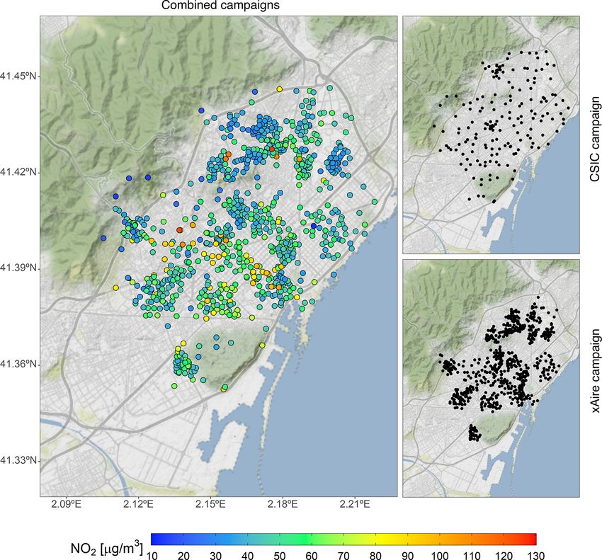
2194              A. Criado et al.: Data fusion uncertainty-enabled methods to map street-scale hourly NO2 in Barcelona

atively easy to implement, and not very demanding regard-              ular geostatistics technique, universal kriging, which consid-
ing computational resources. However, urban areas often                ers the time-aggregated annual mean of an urban model as
present strong NO2 spatial gradients that the official moni-           a basemap (or climatology) to explain the long-term spatial
toring network cannot correctly characterize due to its low            gradients at the street scale, while the time-dependent LCS
spatial representativeness (Vardoulakis et al., 2005; Santiago         network explains the short-term temporal behavior. However,
et al., 2013; Duyzer et al., 2015a). To overcome this lim-             the temporal coverage of their results is restricted to a few
itation and produce accurate surface NO2 maps, urban or                weeks in which measurements are available. Thus, this com-
microscale LUR models rely on low-cost sensors (LCSs),                 promises their ability to systematically estimate hourly NO2
typically restricting the temporal coverage to a few weeks.            exposure levels for extended periods of the order of years.
Works dealing with microscale LUR models have used dif-                   By combining model and observational data, advanced
ferent types of LCSs, including passive dosimeters, which              data fusion methods can provide typically unbiased estimates
report period-averaged concentrations (Perelló et al., 2021a;          of pollutant concentrations at the street scale. However, an-
Su et al., 2009), time-dependent LCSs (Munir et al., 2020;             other piece of information that is of crucial importance is
Weissert et al., 2019), or mobile LCS campaigns (Wang et al.,          the uncertainty in the estimated concentrations, as it can help
2021). Due to the lack of experimental campaigns monitor-              with decision-making or support the design of environmental
ing consistently at high spatial and temporal (hourly) reso-           epidemiological studies (Gryparis et al., 2009). The univer-
lutions over a whole year, current microscale LUR studies              sal kriging methodology provides the error variance of its
typically cannot target the hourly averaged NO2 maximum                predictions, which has already been used as a measure of the
level (200 µg m−3 ) regulated by the 2008 European Union               uncertainty in the data fusion results of NO2 at the street scale
Ambient Air Quality Directive (AAQD; 2008/EC/50).                      (Schneider et al., 2017). However, the validity of the confi-
   Physics-based urban air quality models can generate                 dence intervals and the normality of error distribution in this
hourly pollutant concentration estimates, overcoming the               application remains to be investigated.
temporal limitation of microscale LUR models. Currently,                  Our study presents a data fusion methodology considering
these systems usually consist of the coupling between a re-            a microscale LUR model, in addition to the hourly monitor-
gional chemical transport model, which accounts for the                ing data, to bias correct hourly NO2 estimates of an urban
long-range transport of pollutants, and an urban-scale dis-            dispersion model at a high spatial resolution (20 m × 20 m).
persion model. The latter can be based on semi-empirical               Similar to Schneider et al. (2017), our work also relies on
relations, such as Gaussian dispersion models and mass ex-             the basemap concept. However, contrary to previous stud-
change global parameterizations (e.g., Soulhac et al., 2017;           ies, we have derived it using a microscale LUR model based
Kim et al., 2018; Benavides et al., 2019; Denby et al., 2020;          on 844 samplers from recent passive dosimeter campaigns
Hood et al., 2021), or an obstacle-resolving dispersion model          (Perelló et al., 2021a; Benavides et al., 2019). Thus, the
using computational fluid dynamics (Kwak et al., 2015; Au-             basemap accounts for the spatial patterns, whereas the tem-
vinen et al., 2017). Despite the recent efforts to improve ur-         poral behavior is characterized by the hourly urban model
ban dispersion modeling systems, they are afflicted by per-            output and hourly monitoring data. This approach can be
sistent uncertainties and biases, notably due to the difficulty        very convenient for applying data fusion methods in cities
of prescribing accurate boundary conditions and emissions              for which period-averaged LCS campaigns are available but
at the street scale and reproducing the turbulent phenomena            yearly time-dependent LCS data are lacking, which is usu-
within the urban canopy.                                               ally the case. To assess the benefits of considering such a
   In order to reduce model uncertainties, data fusion meth-           microscale LUR basemap, we compare two different data fu-
ods can be employed to post-process model outputs and ob-              sion methods, namely (i) universal kriging combining hourly
tain more reliable NO2 exposure maps. Several works have               observations with the hourly outputs of a street-scale Gaus-
used monitoring station data to build data fusion methods, ei-         sian dispersion model (i.e., UK-DM) and (ii) universal krig-
ther by relying solely on urban dispersion models to explain           ing combining the above items and the microscale LUR
the spatial distribution (Tilloy et al., 2013) or by adding dif-       model (i.e., UK-DM-LUR). The data fusion methods are ap-
ferent spatial information (e.g., traffic intensity, satellite data,   plied in the city of Barcelona (Spain) for the entire year 2019.
or land use cover) as proxies in addition to the model out-            An original aspect of the present study is the empirical val-
put (Horálek et al., 2006; Chen et al., 2019; Zhang et al.,            idation of the uncertainties based on universal kriging and
2021; Dimakopoulou et al., 2022). In urban areas, the usual            their translation into street-scale probabilities of exceeding
low density of monitoring stations has motivated the devel-            the NO2 hourly and annual regulatory thresholds.
opment of data fusion methods that integrate LCS campaigns                The paper is structured as follows: the observational data
to better explain the spatial distribution of NO2 at the street        and study domain are described in Sect. 2.1. The Gaussian
scale. For instance, the works of Schneider et al. (2017) and          dispersion air quality model, CALIOPE-Urban, used to pro-
Mijling (2020) combine time-resolved LCS hourly data with              duce hourly high-resolution fields of surface NO2 concen-
an urban model output to improve the NO2 characterization              trations is described in Sect. 2.2, while the microscale LUR
at a high-spatial resolution. Schneider et al. (2017) use a pop-       method is explained in Sect. 2.3. A detailed description of the

Geosci. Model Dev., 16, 2193–2213, 2023                                                 https://doi.org/10.5194/gmd-16-2193-2023

A. Criado et al.: Data fusion uncertainty-enabled methods to map street-scale hourly NO2 in Barcelona                        2195

data fusion methods is given in Sect. 2.4. Results of the mi-       els, which implies an estimated uncertainty of ±25 %, as re-
croscale LUR model are presented in Sect. 3.1, and Sect. 3.2        ported in Kuklinska et al. (2015).
discusses the results of the data fusion methodologies. Fi-
nally, conclusions and final remarks are provided in Sect. 4.       2.2   Street-scale air quality model: CALIOPE-Urban

                                                                    Hourly high-resolution concentrations of surface NO2 at the
2     Data and methodology                                          street scale over the city of Barcelona are estimated using
                                                                    the CALIOPE-Urban multiscale air quality model (Bena-
We compare two data fusion methods (UK-DM and UK-                   vides et al., 2019). CALIOPE-Urban accounts for the dis-
DM-LUR; illustrated in Fig. 1). Below we describe each pro-         persion of traffic emissions at high spatial resolution using
cess and dataset used to derive them.                               the R-LINE Gaussian dispersion model (Snyder et al., 2013;
                                                                    Venkatram et al., 2013). As described in more detail in Be-
2.1    Study domain and observational NO2 data                      navides et al. (2019), R-LINE is adapted to street canyons
                                                                    by taking into account road link traffic emissions (Guevara
Barcelona (Fig. 2) is the second most populated city in Spain       et al., 2020), meteorological variables (e.g., wind speed and
and the 10th in Europe, with approximately 1 660 000 inhab-         direction; Monin–Obukhov length and planetary boundary
itants and 102 km2 (∼ 16 300 people per km2 ). It is located        layer height), and building morphology (e.g., building den-
on the northeastern coast of Spain, between the Mediter-            sity and height and street orientation). The chemical balance
ranean Sea and the Collserola mountains. The city has a             between NOx and NO2 is computed based on the generic re-
Mediterranean climate characterized by the dominance of a           action set (Valencia et al., 2018), assuming clear-sky condi-
sea breeze during the warm season, shallow boundary layer           tions and uncoupling chemistry from transport phenomena.
development, and the recirculation of air pollutants (Jorba         In other words, the aging of pollutants is solely a function of
et al., 2004).                                                      wind speed and the distance between the source and recep-
   Hourly NO2 observational data for 2019 are obtained from         tors.
the Catalan Air Pollution Monitoring and Forecasting Net-              At the regional scale, CALIOPE-Urban relies on the
work (XVPCA) measurement points in the Barcelona urban              regional air quality modeling system CALIOPE (Bal-
and surrounding areas. There are 13 stations available on the       dasano Recio et al., 2011) for predicting the urban back-
Barcelona agglomeration (Fig. 2), with a percentage of avail-       ground NO2 concentration. The regional CALIOPE accounts
ability of hourly data greater than 93 %. Gràcia and Eixam-         for the long-range transport of pollutants using three nested
ple are urban traffic monitoring stations, Sagnier, Observa-        domains at increasing resolutions, namely 12 km × 12 km for
tori Fabra, and Jardins are suburban background stations, and       the European region, 4 km × 4 km for the Iberian Peninsula,
the remaining eight correspond to urban background stations.        and 1 km × 1 km for the region of Catalonia (Baldasano Re-
The Observatori Fabra station is not used in our data fusion        cio et al., 2011; Pay et al., 2014). The urban background NO2
methodology since its inclusion significantly degraded the          concentrations obtained with regional CALIOPE are com-
data fusion skills in the urban environment. This is expected,      bined with the R-LINE dispersion results using a dedicated
since the station is located on a hill relatively far from built-   parameterization of the vertical mixing (Benavides et al.,
up areas. In fact, it is not exactly an urban station because       2019).
it measures air pollution above the urban canopy, while the            In this work, CALIOPE-Urban employs a non-uniform
other stations measure pollution within the urban canopy. We        mesh that is refined at the edge of traffic roads and coarser
are aware that, by removing this station, we may lose relevant      in low-gradient regions of NO2 . This type of mesh acceler-
information on the low-NO2 -level regions surrounding the           ates the calculations and reduces memory demand. The re-
city. However, the main goal of our urban model is to char-         fined grid zones have a resolution of 25 m × 25 m, progres-
acterize NO2 exceedances in critical trafficked areas. There-       sively degrading to 500 m × 500 m in the regions of low NO2
fore, we decided to exclude the Observatori Fabra station.          gradients. To facilitate their visualization, these NO2 concen-
   Two different NO2 passive dosimeter experimental cam-            trations are finally interpolated over a uniform mesh, with a
paigns (Fig. 3) are considered to derive the microscale LUR         resolution of 20 m × 20 m. CALIOPE-Urban has been eval-
model, namely the xAire citizen science campaign (Perelló           uated and successfully used in the framework of several im-
et al., 2021a, b) composed of 725 samplers deployed be-             pact studies, including the works of Benavides et al. (2021)
tween 16 February and 15 March 2018 and the 2-week mea-             and Rodriguez-Rey et al. (2022).
surement campaign of the Institute of Environmental As-
sessment and Water Research – Spanish National Research             2.3   Microscale LUR model using gradient boosting
Council (IDAEA-CSIC) that deployed 175 NO2 samplers                       machine (GBM)
across Barcelona during February and March 2017 (Bena-
vides et al., 2019). Both campaigns used Palmes-type NO2            A nonlinear microscale LUR model based on passive
diffusion tubes (Palmes et al., 1976) to sample the NO2 lev-        dosimeter campaigns is used to produce an observation-

https://doi.org/10.5194/gmd-16-2193-2023                                              Geosci. Model Dev., 16, 2193–2213, 2023
2196             A. Criado et al.: Data fusion uncertainty-enabled methods to map street-scale hourly NO2 in Barcelona

Figure 1. Workflow of the two studied data fusion methodologies. Hourly data from monitoring stations are combined with hourly dispersion
model results (UK-DM) and the time-invariant microscale LUR basemap (UK-DM-LUR). PBL stands for planetary boundary layer.

based climatological view of the NO2 concentrations at a               and temperature) and also allows the combining of both cam-
high spatial resolution over Barcelona. While the monitor-             paigns, producing a dataset of 844 samplers on which the
ing stations and the urban dispersion model provide informa-           microscale LUR model relies. Note that the microscale LUR
tion on the pollutants’ short-term temporal behavior, the mi-          model is trained using experimental campaigns deployed in
croscale LUR basemap (long-term mean) remains constant                 February and March. As a result, even though the annualiza-
in time. Its main goal is to provide reliable long-term spatial        tion process corrects the NO2 levels and the predictors are
variability patterns of NO2 at a high resolution, using obser-         expressed as annual averages, the captured spatial gradients
vational data and other urban information.                             may still have a significant seasonal bias.
    The target variable of the microscale LUR model is the                The potential predictors of the microscale LUR model are
time-averaged concentrations of the two different NO2 ex-              shown in Table 1. The geometric variables are calculated
perimental campaigns described in Sect. 2.1 and represented            from the Institut Cartogràfic i Geològic de Catalunya (ICGC,
in Fig. 3. We have discarded the xAire samplers related to             2019) and Plan Nacional de Ortografía Aérea (PNOA, 2020).
playgrounds and classrooms, so we are using the remain-                Traffic-related predictors consist of traffic density (t) for dif-
ing 669. In order to combine the xAire and IDAEA-CSIC                  ferent circular buffer sizes. With a being the radius of the
campaigns, we have annualized both, following the proce-               buffer, ta is computed following Eq. (1; expressed in vehi-
dure described in Perelló et al. (2021b). For each station, an         cles per m s−1 ):
adjustment factor is computed as the ratio between the ob-
                                                                              n
served 2017 annual mean and the average over the period of                    X
                                                                       ta =         AATi · la,i ,                                    (1)
the experimental campaign. Then, the average of this factor
                                                                              i=1
over all stations is used to scale all passive samplers to the
2017 annual mean. This scaling assumes that the ratio does             where i represents the street segment, n is the number of
not depend on the location and can be applied to all sam-              street segments over the circular area of π a 2 , li is the length
plers. Despite adding some noise to the experimental results,          of the street segment i within the buffer of radius a, and AATi
it corrects the bias induced by environmental conditions (e.g.,        is the annual average traffic of the street segment i (expressed
wind speed, atmospheric stability, precipitation, radiation,           in vehicles per second). The ta predictors associated with the

Geosci. Model Dev., 16, 2193–2213, 2023                                                     https://doi.org/10.5194/gmd-16-2193-2023
A. Criado et al.: Data fusion uncertainty-enabled methods to map street-scale hourly NO2 in Barcelona                         2197

                                                                    tant feature, while monitoring the RMSE in cross-validation
                                                                    (CV). The goal is to obtain the simplest model with the low-
                                                                    est RMSE to gain generalization and interpretability. The fi-
                                                                    nal microscale LUR model includes the following eight pre-
                                                                    dictors: average building density, traffic buffers of 25 and
                                                                    100 m, traffic-scaled variable s, all the annually averaged
                                                                    data from the regional CALIOPE modeling system (NO2 , the
                                                                    planetary boundary layer height, and the wind speed), and the
                                                                    NO2 annual mean from CALIOPE-Urban.
                                                                       To account for nonlinear relations among the predictors
                                                                    and the target variable, we used the gradient boosting ma-
                                                                    chine (GBM) algorithm implemented in the R package gbm
                                                                    (Greenwell et al., 2022). GBM is a popular machine learn-
                                                                    ing algorithm (Natekin and Knoll, 2013) that has shown
                                                                    excellent results in terms of accuracy and generalization
                                                                    when compared to other learning algorithms (Caruana and
                                                                    Niculescu-Mizil, 2006). The GBM hyperparameters (shrink-
                                                                    age rate, interaction depth, minimum observation per node,
                                                                    and bag fraction) are optimized based on the minimum mean
                                                                    cross-validated error and a grid search algorithm. Addition-
                                                                    ally, following the work of Chen et al. (2019), we exploit the
                                                                    potential spatial correlation of the GBM residuals by inter-
                                                                    polating and adding them to the predicted values. The inter-
                                                                    polation is done with ordinary kriging (Wackernagel, 2003).
                                                                       One could think that skipping over the LUR computation
Figure 2. Domain of study and location of the referenced mon-       by directly using all of its time-invariant information (passive
itoring stations. The map has been generated using the ggplot2
                                                                    dosimeter campaigns, urban geometry, traffic-related data,
(Wickham, 2016) and ggmap (Kahle and Wickham, 2013) R pack-
                                                                    and annually averaged model results) as covariates in the
ages (R Core Team, 2013) and data from OpenStreetMap. © Open-
StreetMap contributors 2017, distributed under the Open Data Com-   universal kriging methodology would simplify the workflow.
mons Open Database License (ODbL) v1.0. Map tiles are by © Sta-     However, there are two main drawbacks to doing so. On the
men Design, under a Creative Commons Attribution (CC BY 3.0)        one hand, in contrast to GBM, universal kriging assumes
license.                                                            linear relations between covariates and the observed NO2 ,
                                                                    which is not necessarily true for this case. On the other hand,
                                                                    when considering a large number of covariates with only
smaller buffers (5, 10, and 15 m) have highly skewed distri-        12 monitoring stations, strong spurious correlations lacking
butions, given that most values across the map are null. To         physical meaning are prone to happen, which drive the fi-
avoid training the microscale LUR with skewed predictors,           nal solution wrongly (Hengl et al., 2007). Thus, gathering all
we introduce the traffic-scaled variable s here, which com-         static information into a single LUR covariate offers more ro-
bines all buffers as follows:                                       bust results, while permitting the addition of predictors using
     1 X ta                                                         nonlinear regression models.
s=              ,                                        (2)
     N a π a2
                                                                    2.4   Universal kriging as a data fusion methodology for
where N is the number of buffers (12 in our case). Traf-                  spatial bias correction
fic data are extracted from the road link traffic network of
the HERMESv3 bottom-up emission model (Guevara et al.,              The microscale LUR model and the hourly CALIOPE-Urban
2020). We also considered NO2 , the planetary boundary              outputs are combined with observational NO2 data from the
layer height, and the wind speed annual averages from the           monitoring stations using the geostatistical technique of uni-
regional air quality modeling system CALIOPE as potential           versal kriging, which is commonly used for spatial interpo-
predictors, together with the NO2 annual mean from the air          lation. This methodology predicts a random variable Z at
quality model CALIOPE-Urban.                                        a target point x, based on a combination between a (multi-
   A recursive feature elimination method has been applied to       )linear regression analysis with external variables f , referred
remove highly correlated or uninformative features. We have         to as covariates, and a pure spatial interpolation considering
used the simple backward-selection algorithm implemented            the autocorrelation structure of the regression residuals. In
in the R package caret (Kuhn, 2008), which starts with the          our case, the variable Z corresponds to the monitoring data,
full-featured model and gradually removes the least impor-          while the covariates are CALIOPE-Urban and our microscale

https://doi.org/10.5194/gmd-16-2193-2023                                              Geosci. Model Dev., 16, 2193–2213, 2023
2198              A. Criado et al.: Data fusion uncertainty-enabled methods to map street-scale hourly NO2 in Barcelona

Figure 3. Sampler locations of the two different NO2 experimental campaigns used to train the microscale LUR model. The left panel shows
the NO2 values and the locations of the combined campaigns. The top-right and bottom-right panels show the CSIC and xAire campaign
locations, respectively. The color scale refers to the 2017 annualized NO2 values (in µg m−3 ). The map has been generated using ggplot2
(Wickham, 2016) and ggmap (Kahle and Wickham, 2013) R packages (R Core Team, 2013) and data from OpenStreetMap. © OpenStreetMap
contributors 2017, distributed under the Open Data Commons Open Database License (ODbL) v1.0. Map tiles are by © Stamen Design, under
a Creative Commons Attribution (CC BY 3.0) license.

Table 1. The microscale LUR model contemplates the use of these 21 potential predictors.

     Type                        No.     Variable                                Resolution
                                 1       Average building density
                                 2       Average building height
     Urban geometric                                                             Square buffer of 250 m × 250 m
                                 3       Maximum building height
                                 4       Standard deviation building height
     Traffic related             5–16    Simulated vehicular traffic densities   Circular buffers of 5, 10, 15, 25, 50, 100, 300, 500,
                                                                                 1000, 2000, 3000, and 4000 m of radius
                                 17      Traffic scaled                          Linear combination of the buffers above
     Output from the             18      NO2                                     Uniform mesh of 1 km × 1 km
     regional modeling system    19      Planetary boundary layer height
     CALIOPE (lowest layer)      20      Wind speed
     Output from the             21      NO2                                     Non-uniform mesh (25 m × 25 m to 500 m × 500 m)
     CALIOPE-Urban model

Geosci. Model Dev., 16, 2193–2213, 2023                                                    https://doi.org/10.5194/gmd-16-2193-2023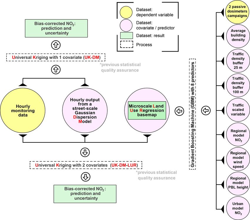
A. Criado et al.: Data fusion uncertainty-enabled methods to map street-scale hourly NO2 in Barcelona                           2199

LUR model. A simple (multi-)linear regression model is con-            Zl (x) and σl2 (x) are the prediction and variance in the log
venient here, given the low number (12) of available moni-             space, respectively.
toring stations within the computational domain. Universal                Assuming a normal distribution of the error, the probabil-
kriging assumes the following relation (Cressie, 1993):                ity of exceedance (P) of a certain limit value (L) can be com-
              L                                                        puted as follows (Horálek et al., 2008):
              X
Z(x) =               al fl (x) + R(x),                           (3)                               !
               l=0                                                                       L − Ẑ(x)
                                                                       P(x) = 1 − F                  ,                             (7)
where L equals 1 in the UK-DM approach and 2 in the UK-                                    σ̂ (x)
DM-LUR, al are the non-zero coefficients from the (multi-
)linear regression between the observations and the covari-            where F is the normal cumulative distribution function.
ates fl (with f0 (x) = 1 by convention), and R(x) is the resid-
ual random field. The deterministic part of the variable Z is          2.4.1   Statistical metrics to evaluate data fusion skills
explained by a linear combination of the covariates, while
the residual random field is considered to have zero mean              Statistical performance is assessed by leave-one-out cross-
and to be spatially autocorrelated. The main advantage of this         validation (LOOCV), which consists of performing the data
method is that, depending on the strength of the correlation           fusion by considering all of the monitoring stations, except
between covariates and observations, universal kriging gives           for one that is kept to cross-validate the results. For each
more weight either to the (multi-)linear regression or to the          LOOCV, we present the coefficient of efficiency (COE), the
spatial interpolation of the residuals (Hengl, 2009), thus pro-        root mean square error (RMSE), the mean bias (MB), and the
viding a robust data fusion method that adapts to the quality          correlation coefficient (r), defined as follows:
of the model output.                                                             Pk
                                                                                      |Mi − Oi |
   As a Gaussian process, universal kriging estimates the              COE = 1 − Pi=1
                                                                                   k
                                                                                                                                    (8)
variance of its predictions (σ 2 ) coming from both the (multi-                    i=1 |Oi − O|
                      2
)linear regression (σMLR                                     2)
                           ) and the spatial interpolation (σSI                 k
                                                                             1X
steps, as follows:                                                     MB =        Mi − Oi                                          (9)
                                                                             k i=1
               m
               X                             L
                                             X
σ 2 (x) =             wα · γR (xα − x) +                                          k
                                                   λl fl (x),    (4)        1 X        Mi − M      Oi − O
               α=1                           l=0                       r=                                                        (10)
               |           {z            }   |     {z     }               k − 1 i=1       σM           σO
                            2
                           σSI                    2
                                                 σMLR                           v
                                                                                u k
                                                                                u1 X
where m is the number of monitoring stations, wα are the               RMSE = t          (Mi − Oi )2 ,                           (11)
spatial interpolation weights associated with each measure-                        k i=1
ment point, λl are the L + 1 Lagrangian multipliers used to
minimize the variance error, and γR (xα − x) stands for the            where k is the total number of observations, Oi and Mi are
variogram which characterizes the spatial structure of the             the observed and modeled i values, respectively, O and M
residuals (Chiles and Delfiner, 1999). Thus, the variance of           are their respective means, and σO and σM refer to their stan-
a prediction reflects how far the unmeasured location is from          dard deviation.
the observation points and from the feature space in which
the regression model has been calibrated, i.e., the extrapola-         2.4.2   Spatial autocorrelation structure of NO2 levels
tion effect (Hengl, 2009). Our universal kriging implemen-
                                                                       In the universal kriging context, the variogram describes the
tation relies on the R package gstat (Pebesma, 2004; Gräler
                                                                       spatial autocorrelation structure of the residual random field.
et al., 2016).
                                                                       In our case, the limited number of monitoring stations makes
   To normalize the distribution of the NO2 data and to en-
                                                                       it challenging to extract a meaningful spatial structure. For
sure positive predicted values, we have applied the universal
                                                                       this reason, we estimate the residual variogram based on
kriging technique described above after transforming NO2
                                                                       the dosimeter campaigns. This decision, however, entails a
data into the log space. However, the results need to be
                                                                       substantial limitation due to the assumption of a static var-
back-transformed to the original scale. Following the work
                                                                       iogram. We rely only on the IDAEA-CSIC campaign (dis-
of Cressie (1993), the back-transformation is performed as
                                                                       carding the xAire campaign for the variogram derivation) to
follows:
                                                                       avoid extra premises for the combination of campaigns. Ad-
Ẑ(x) = exp(Zl (x) + σl2 (x)/2),                                 (5)   ditionally, we considered an isotropic variogram. All of these
σ̂   2
         (x) = (exp(σl2 (x)) − 1) · exp(2 · Zl (x) + σl2 (x)),   (6)   postulates impact the variance error estimated by universal
                                                                       kriging (Brus and Heuvelink, 2007). To assess the impact of
where Ẑ(x) and σ̂ 2 (x), respectively, represent the back-            such assumptions, an analysis of the estimated variance in
transformed prediction and variance at the target point, while         LOOCV is carried out in Sect. 3.2.

https://doi.org/10.5194/gmd-16-2193-2023                                                 Geosci. Model Dev., 16, 2193–2213, 2023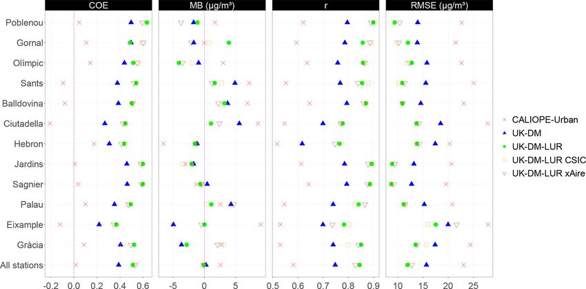
2200             A. Criado et al.: Data fusion uncertainty-enabled methods to map street-scale hourly NO2 in Barcelona

   The variogram is fitted using the Matérn model with
Stein’s parameterization implemented in the R package au-
tomap (Hiemstra et al., 2009), setting the smoothing param-
eter κ = 0.2. The resulting variogram model is characterized
by a 5 × 10⁻² partial sill, 3 × 10⁻⁵ nugget, and a range of
620 m. Following the work of Denby et al. (2007), we have
optimized the range value to minimize the RMSE of univer-
sal kriging. The range estimates the distance at which the
data are no longer correlated. To optimize it, we performed
an hourly LOOCV by varying the range from 1 to 10 km for
                                                                    Figure 4. Scheme of the outer 10-fold CV and the inner 4-fold CV
every 1 km, while keeping all other model parameters con-           applied for the GBM training.
stant. We obtained the best results for the range of 5 km,
which improved the r coefficient by 4 %, the COE by 14 %,
and the RMSE by −9 % on average over all monitoring sta-            3     Results and discussion
tions, compared to the UK-DM-LUR methodology that used
the original range of 620 m.                                        The results are organized into two sections. First, in Sect. 3.1,
                                                                    we estimate the microscale LUR model performance and
2.4.3   Statistical quality assurance of the (multi-)linear
                                                                    present the obtained NO2 basemap. Second, in Sect. 3.2, the
        regression
                                                                    data fusion methodologies are discussed in terms of statisti-
The correlation coefficient (r) and the regression coeffi-          cal performance, uncertainty quantification, and exceedance
cient (slope) of the regression model between covariates            probability maps. All the maps presented in this section
(CALIOPE-Urban and the microscale LUR model) and ob-                have been generated using the ggplot2 (Wickham, 2016) and
servations are checked before the covariates are included in        ggmap (Kahle and Wickham, 2013) R packages (R Core
the universal kriging workflow (as indicated in Fig. 1). If a       Team, 2013) and data from Open Data BCN (Ajuntament
covariate shows a low correlation (p value > 0.05) with the         de Barcelona, 2019) and OpenStreetMap (© OpenStreetMap
observations at a specific hour, then it is not considered in       contributors 2017, distributed under the Open Data Com-
the regression model, as in the works of Zhang et al. (2021)        mons Open Database License (ODbL) v1.0. Map tiles are by
and Oh et al. (2021). Additionally, if none of the covariates       © Stamen Design, under a Creative Commons Attribution
shows a significant correlation, then we use both covariates        (CC BY 3.0) license).
to build the regression model. However, to avoid nonphysical
                                                                    3.1     Microscale LUR model
hourly maps, the covariates are used only if their regression
coefficient is positive, as suggested by Denby et al. (2007).
                                                                    3.1.1    Performance assessment
In case all of the regression coefficients are negative, or there
are fewer than four observations available in a specific hour,      The GBM-based microscale LUR model is evaluated using
universal kriging is not performed, and the results of the data     two nested K-fold CVs, with the inner one for tuning the
fusion method are directly the raw dispersion–model output.         model (training–validation set) and the outer one for testing
Following the above criteria, the percentage of cases with          the model on different parts of the dataset (test set). Such a
fewer than four monitoring observations is relatively small,        procedure aims at giving a reliable estimate of the expected
0.034 % (3 h), and is the same for each kriging application.        performance. We use an outer 10-fold CV and an inner 4-
For the UK-DM methodology, 14.11 % of the hours have not            fold CV, as illustrated in Fig. 4. The tuning of the model is
been corrected due to negative regression coefficients. On the      performed through a grid search over the following hyperpa-
other hand, for the case of UK-DM-LUR, only 1.47 % of the           rameters: shrinkage rate (with values ranging from 0.001 to
hours have been discarded due to a negative regression coeffi-      0.05 every 0.001), the interaction depth (from 1 to 4 every 1),
cient in both covariates. As Benavides et al. (2019) identified,    the minimum observation in a node (from 5 to 15 every 1),
the poor skills of the urban model are attributed to low wind       and the bag fraction (0.5 and 0.65).
speeds and atmospheric stability situations, which cause the           The results are given in Table 2, together with the per-
performance of the mesoscale model to decrease. Concern-            formance reference of the annual mean NO2 concentration
ing the static microscale LUR basemap, the poor correlation         obtained directly from CALIOPE-Urban. As explained in
on an hourly basis is associated with hours that significantly      Sect. 2.3, we exploit the spatial autocorrelation of the LUR
deviate from the average behavior.                                  residuals to improve its estimation. To do so, the microscale
                                                                    LUR residuals at the training locations are interpolated at the
                                                                    test locations by applying an ordinary kriging. Then, they are
                                                                    added to the predictions to obtain the corrected results (see
                                                                    values for “test set adding the residuals” in Table 2).

Geosci. Model Dev., 16, 2193–2213, 2023                                              https://doi.org/10.5194/gmd-16-2193-2023
A. Criado et al.: Data fusion uncertainty-enabled methods to map street-scale hourly NO2 in Barcelona                             2201

Table 2. Statistical results of the microscale LUR model in nested CV. The 2017 annual mean concentration of NO2 of the raw dispersion
model (CALIOPE-Urban) is also shown. The parameter n stands for the number of data points used to compute the statistics.

             Model                                                                n    COE         MB        r     RMSE
                                                                                              (µg m−3 )          (µg m−3 )
                                       Training–validation set                  7600   0.30       0.15    0.69       11.38
             Microscale LUR            Test set without adding the residuals     840   0.24       0.22    0.62       12.17
                                       Test set adding the residuals             840   0.27      −0.27    0.64       11.87
             Raw CALIOPE-Urban         Annual mean                              840    0.13      −0.81    0.54       13.68

    Table 2 shows that the microscale LUR model signifi-                of samplers to derive a robust microscale LUR is presented
cantly improves the CALIOPE-Urban results. Also, the ad-                in Appendix A.
dition of the residuals slightly increases the statistical perfor-
mance. The training–validation set results are not perfectly            3.1.2    Microscale LUR basemap
fitted and are only slightly better than the test set results, in-
dicating that the microscale LUR is not overfitted and has              We proceed to train the microscale LUR model with the
good capabilities for the prediction of unseen data.                    residual correction using all available sampling sites. Fig-
    In Fig. 5, we show the scatterplots of the CALIOPE-Urban            ure 6 compares the long-term NO2 patterns from the mi-
annual mean and the test set results with and without adding            croscale LUR basemap (Fig. 6a) with the NO2 2019 annual
the residuals, along with the observational uncertainty ranges          mean of CALIOPE-Urban (Fig. 6b). Notice that the goal of
indicated by the dashed red lines (±25 %, according to Kuk-             the basemap is to correct the long-term spatial variability in
linska et al., 2015). Although a large portion of the predicted         NO2 . Thus, Fig. 6 highlights the differences in spatial pat-
values for the microscale LUR model with the residual cor-              terns rather than differences in absolute NO2 values. The re-
rection lies within the uncertainty range, difficulty can be ob-        sulting basemap shows a qualitatively consistent NO2 distri-
served in predicting values of NO2 higher than 80 µg m−3 .              bution; the major trafficked roads of the city and the port area
We attribute this behavior to not only the limited number of            are the most polluted locations, while the Collserola moun-
points in this range, which can weaken the model training,              tains and the sea bordering the city have moderate NO2 lev-
particularly in the nested CV context, but also to the already          els. Although both figures show similar NO2 patterns, local
poor predictive skills of CALIOPE-Urban in this concentra-              differences from experimental information can be observed
tion range (as seen in Fig. 5a).                                        in Fig. 6a. For instance, there is a noticeable increase in NO2
    Comparing these results with previous works, the result-            levels for the microscale LUR basemap in the mountainous
ing correlation coefficient (r) is lower than a LUR model               northwestern area of the study domain. This artifact is proba-
fitted with the xAire campaign data (r = 0.74 in LOOCV),                bly caused by the spatial distribution of the passive dosimeter
as reported in Perelló et al. (2021a). However, Perelló et al.          campaigns (Fig. 3), which poorly cover this region. The NO2
(2021a) used only 370 outdoor sampling sites out of the                 overprediction of this area is not reflected in the statistical
669 available. They excluded samplers close to traffic and              evaluation of the data fusion since we deliberately omitted
street intersections, achieving a skilled urban LUR model.              the monitoring station located in this area. We excluded this
Even if the r coefficient is slightly lowered, we have consid-          station to improve the data fusion model’s ability to capture
ered all outdoor sampling sites (along with the IDAEA-CSIC              NO2 exceedances in built-up areas, which is the main goal
campaign) to capture, as much as possible, the NO2 spatial              of the urban model. As further shown in the statistical re-
trends. On the other hand, the work of Munir et al. (2020) re-          sults, considering extensive passive dosimeters information
ported a microscale LUR model based on 40 time-dependent                through the microscale LUR model avoids relying only on
LCSs with slightly lower performance in the CV than the                 the urban model to describe the NO2 gradients and signifi-
present one (r = 0.56). Moreover, Munir et al. (2020) also              cantly improves the data fusion methodology.
reported a r value of 0.53 when the nonlinear LUR model                    The influence of each predictor in the final microscale
is based on the combination of 188 period-averaged and 40               LUR model has been computed based on the methodology
time-dependent LCSs. A key aspect of the present data fu-               proposed by Friedman (2001) and implemented in the R
sion methodology is that the microscale LUR model results               package gbm (Greenwell et al., 2022), in which the relative
explain better the annualized passive dosimeter campaigns               importance of each variable is associated with the reduction
compared to the reference CALIOPE-Urban annual mean.                    in the GBM cost function. Given the chosen set of predictors,
Therefore, they are subsequently considered to be a covariate           the most influential variable is the NO2 CALIOPE-Urban an-
in the universal kriging methodology, as further explained in           nual mean with a relative importance of 25.1 %, followed by
Sect. 3.1.2. An assessment regarding the necessary number               17.7 % for the traffic scaled variable and 15.7 % for the aver-

https://doi.org/10.5194/gmd-16-2193-2023                                                  Geosci. Model Dev., 16, 2193–2213, 2023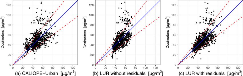
2202             A. Criado et al.: Data fusion uncertainty-enabled methods to map street-scale hourly NO2 in Barcelona

Figure 5. (a) Raw annual mean of CALIOPE-Urban NO2 concentrations, (b) microscale LUR model results, without the interpolated
residuals, and (c) microscale LUR model results, with the interpolated residuals, versus the annualized passive dosimeter campaigns. These
figures use the test sets in which the performance of the microscale LUR model has been assessed. The dashed red lines report passive
dosimeter uncertainty (±25 %), and the identity line is represented in blue. The statistical results are shown in Table 2.

Figure 6. (a) Resulting microscale LUR basemap using all available sampling sites and adding the interpolated residuals. (b) The 2019
annual mean concentration of NO2 of the raw dispersion model CALIOPE-Urban.

age building density. The other predictors exhibited a relative        First, the output of the urban dispersion model CALIOPE-
influence under the 15 %, with the NO2 CALIOPE regional                Urban is merged with the monitoring data using univer-
annual mean as the lowest one with 4.3 %.                              sal kriging, named UK-DM. Second, the microscale LUR
                                                                       basemap is added as a covariate in the universal kriging
3.2     Data fusion methodologies                                      workflow, named UK-DM-LUR.
                                                                          Hourly statistical results for the raw CALIOPE-Urban,
3.2.1    Statistical evaluation                                        UK-DM, and UK-DM-LUR models are shown in Fig. 7 for
                                                                       each monitoring station using all available data of 2019.
In order to quantify the added value of including the mi-              UK-DM and UK-DM-LUR results have been computed in
croscale LUR basemap in the data fusion methodology, two               LOOCV, as explained in Sect. 2.4. Gràcia and Eixample
different post-processes (see Fig. 1) have been carried out.

Geosci. Model Dev., 16, 2193–2213, 2023                                                  https://doi.org/10.5194/gmd-16-2193-2023
A. Criado et al.: Data fusion uncertainty-enabled methods to map street-scale hourly NO2 in Barcelona 2203
Figure 7. Statistical results for each station after applying UK-DM and UK-DM-LUR to 2019 hourly data in LOOCV. In addition, we show
the statistical results for the CALIOPE-Urban estimates at each station. All stations refer to the average over all stations.
are the urban traffic monitoring stations, and the last row in Table 3. Percentages of observations falling in the ±σ̂ , ±2σ̂ , ±3σ̂
Fig. 7 corresponds to the average results over all stations. confidence intervals, using all stations in LOOCV during 2019.
This figure shows that the hourly scale post-processing con- Confidence intervals are computed based on the hourly predicted
sistently improves all studied statistical metrics at all moni- values and their standard deviation.
toring stations, regardless of their type. Moreover, adding the
±1σ̂ ±2σ̂ ±3σ̂
microscale LUR basemap as a covariate (UK-DM-LUR) fur-
ther improves the spatial correction at all stations and for all Nref 68 % 95 % 99,7 %
statistical metrics, except for the MB, which does not have UK-DM 47.9 % 78.0 % 91.3 %
a clear trend. A negative COE value reflects a poor predic- UK-DM-LUR 51.2 % 81.3 % 92.9 %
tive capacity, so we highlight that both data fusion methods
achieve a positive COE at all considered stations. Almost all
stations show a positive MB for CALIOPE-Urban, indicat-
ing a general overestimation of the model, while UK-DM while we know that, in the urban scale, the NO2 autocorre-
and UK-DM-LUR present almost null MB averaged over lation structure may vary significantly, depending on the di-
all stations. The overestimation of CALIOPE-Urban in the rection with respect to traffic road links. These assumptions
monitoring stations may seem contradictory, with the nega- directly impact the error variance estimated by the universal
tive bias presented in Table 2 for the passive dosimeter cam- kriging, σ̂ 2 . Considering that the interpolation error is nor-
paigns. However, this could indicate that the highest NO2 mally distributed (Nref ), the observation at a specific monitor-
values in Barcelona are not routinely monitored, as already ing station when performing a LOOCV should be within ±σ̂
pointed out in the work of Duyzer et al. (2015b). Regard- of the predicted value for 68 % of the time, while being 95 %
ing the RMSE, the averaged reduction between CALIOPE- and 99.7 %, respectively, for ±2σ̂ and ±3σ̂ , as indicated in
Urban and UK-DM is about 32 % and 24 % between UK- Table 3. To assess the normality of these distributions, Ta-
DM and UK-DM-LUR. For the r coefficient, an averaged ble 3 reports an empirical validation of the percentage of ob-
improvement of 29 % between CALIOPE-Urban and UK- servations falling within the corresponding error range, again
DM is observed, while the improvement between UK-DM computed in LOOCV. These percentages show that the un-
and UK-DM-LUR is 13 %. certainty is underpredicted for both methods. However, the
overconfident UK-DM-LUR results are slightly better than
3.2.2 Uncertainty quantification the UK-DM ones.
To better understand the behavior of uncertainty estimates,
The uncertainty in the universal kriging predictions is esti- in Fig. 8 we show the probability density functions (PDFs) of
mated from the (multi-)linear regression and the spatial inter- the hourly bias, normalized by the error standard deviation
polation variances, as formulated in Eq. (4). The spatial inter- σ̂ , for UK-DM and UK-DM-LUR, using all studied moni-
polation is based on the variogram, which has been modeled toring stations in LOOCV over all available hours in 2019.
from a period-averaged passive dosimeter campaign; thus, it The error PDFs have normal trends with a slightly negative
assumes a static behavior, as pointed out in Sect. 2.4.2. Addi- skew and are overconfident, in accordance with Table 3. Both
tionally, the variogram is considered isotropic for simplicity, methodologies, especially UK-DM, exhibit negative skew-
https://doi.org/10.5194/gmd-16-2193-2023 Geosci. Model Dev., 16, 2193–2213, 20232204 A. Criado et al.: Data fusion uncertainty-enabled methods to map street-scale hourly NO2 in Barcelona
Table 4. Statistical results using the 12 monitoring stations after
applying UK-DM and UK-DM-LUR directly to the annual averages
in LOOCV.
COE MB r RMSE
(µg m−3 ) (µg m−3 )
UK-DM 0.25 0.20 0.74 3.93
UK-DM-LUR 0.38 0.37 0.83 3.24
Figure 10 presents the NO2 annual mean, its associated
relative uncertainty, and the probability map of values ex-
ceeding the NO2 annual limit value of 40 µg m−3 (AAQD
2008/EC/50) for both UK-DM and UK-DM-LUR method-
ologies. The annual mean levels combining the raw model
with the monitoring stations data (UK-DM; Fig. 10a) have
Figure 8. PDF of the hourly bias, normalized by the universal krig-
similar trends to the raw CALIOPE-Urban (Fig. 6b). How-
ing standard deviation, for all monitoring stations in LOOCV dur-
ever, pollution levels are significantly reduced. Adding the
ing 2019. The PDFs correspond to the reference normal distribution
(Nref ), UK-DM, and UK-DM-LUR hourly results. passive dosimeter information through the microscale LUR
basemap (UK-DM-LUR; Fig. 10d) slightly increases NO2
concentrations, particularly in the city center and secondary
ness. This is because the corrected model struggles to capture roads, where the microscale LUR basemap (Fig. 6a) exhibits
the infrequent high-pollution peaks, tending to underestimate steeper NO2 gradients than CALIOPE-Urban (Fig. 6b).
them significantly instead. Thus, negative biases (Mh < Oh ) As expected, the areas surrounding the monitoring sta-
are rare but stronger. On the other hand, the model tends tions (presented in Fig. 2) show lower relative uncertainty,
to overpredict moderate observed values slightly. Therefore, as can be seen in Fig. 10b and e. The higher uncertainty re-
positive biases (Mh > Oh ) are more frequent and less severe. gions, on the other hand, correspond to areas far from the
In agreement with the overall null bias, the rare strong under- monitoring sites, and areas with extreme concentration lev-
estimations are compensated by frequent moderate overesti- els, which causes an extrapolation effect in the regression
mations. model. When comparing the two uncertainty maps (Fig. 10b
In addition, in Fig. 9, the PDFs are computed by split- and e), UK-DM-LUR has regions with higher relative uncer-
ting the observed NO2 concentration levels in three different tainty than UK-DM. This behavior is due to the addition of
ranges, namely less than 40 µg m−3 , greater than 100 µg m−3 , the microscale LUR covariate, which increases the standard
and between 40 and 100 µg m−3 . These PDFs allow us to deviation associated with the regression model. In addition,
study the behavior of the error distribution for different NO2 some localized regions of high uncertainty can be observed
values. This figure shows that larger concentration levels tend in Fig. 10e. They are associated with the locations of the pas-
to be underestimated, while the smaller ones are overesti- sive dosimeters and trafficked roads, where the microscale
mated. In all ranges and for both methodologies, the normal LUR covariate has caused an increase in NO2 concentrations,
trends of the error PDFs are conserved, with the intermediate thereby raising the level of extrapolation in the regression
ranges being the closest to the theoretical normal distribu- model. The high uncertainty values in the upper-left corner
tion. of Fig. 10b and e correspond to the low NO2 levels pre-
dicted in the Collserola mountains. These high-uncertainty
3.2.3 Street-scale maps values can be reduced by considering the Observatori Fabra
station, which is located in this area. However, as explained
We first analyze the annual mean concentration levels of in Sect. 2.1, we excluded this station since its inclusion de-
NO2 . Table 4 presents the evaluation in LOOCV of the re- creases the data fusion model’s ability to predict high NO2
sults post-processed by the UK-DM and the UK-DM-LUR values in critical trafficked areas.
methodologies applied directly to the 2019 annual mean. Regardless of the data fusion method, the most polluted re-
The presented statistics are computed using a single NO2 - gions correspond to probabilities exceeding the annual limit
averaged value for each station. The annually based statistics above 0.7, as shown in Fig. 10c and f. When considering
are similar to the hourly results shown in Fig. 7. However, the UK-DM-LUR method, 13 % of the Barcelona munici-
there is a substantial drop in the RMSE associated with the pality area has a 0.7 or higher probability of exceeding the
bias compensation when averaging the hourly data. annual limit, and this percentage rises to 30 % when consid-
ering probabilities equal to or higher than 0.5. The Eixam-
Geosci. Model Dev., 16, 2193–2213, 2023 https://doi.org/10.5194/gmd-16-2193-2023A. Criado et al.: Data fusion uncertainty-enabled methods to map street-scale hourly NO2 in Barcelona 2205
Figure 9. PDFs by observed NO2 ranges of the hourly bias, normalized by the standard deviation error, for all monitoring stations in LOOCV
during 2019 for (a) UK-DM and (b) UK-DM-LUR applications.
ple district, which is the most polluted, while being the most with a probability equal to or higher than 0.5 and 6 % in the
populous and densely populated (approximately 270 000 in- case of 0.7.
habitants and 36 000 inhabitants per square kilometer, ac-
cording to Ajuntament de Barcelona, 2019), has 95 % of its
area exceeding the annual limit, with a probability equal to or 4 Conclusions
higher to 0.5 and 69 % in the case of 0.7. Thus, significant ev-
The present work assesses the added value of including a
idence indicates that the NO2 annual legal limit was broadly
microscale LUR basemap into a data fusion method to ob-
exceeded in Barcelona in 2019. Stronger evidence could be
tain spatially bias-corrected urban maps of NO2 at the hourly
obtained by reducing the uncertainty associated with the re-
scale. To do so, we have compared two different data fusion
sults, either by using a better-correlated urban model or by in-
methods, namely (i) merging an urban dispersion model with
creasing the monitoring system’s coverage. To test a more re-
the observational data coming from 12 monitoring stations,
strictive threshold, we have analyzed the annual exceedance
using universal kriging (UK-DM), and (ii) adding a nonlinear
probability maps using the recommended WHO 2021 an-
microscale LUR model as a covariate in the kriging workflow
nual limit of 10 µg m−3 (WHO, 2021), obtaining probabili-
based on the GBM algorithm (UK-DM-LUR). The compari-
ties above 0.9 across the domain for both methodologies (not
son is based on the statistical performance in LOOCV at each
shown here).
monitoring station, the resulting NO2 maps, and their associ-
Figure 11 presents the NO2 prediction at a specific hour,
ated uncertainty.
its associated relative uncertainty, and the exceedance prob-
The statistical performance of the microscale LUR model
ability map based on the 200 µg m−3 NO2 hourly threshold
has been assessed using a comprehensive nested CV. As
(AAQD 2008/EC/50) for the UK-DM-LUR methodology.
expected, the obtained microscale LUR basemap (r =
The goal is to illustrate that, apart from studying the long-
0.64; RMSE = 11.87 µg m−3 ) outperformed the raw annu-
term NO2 values, the present methodology can also be used
ally averaged dispersion model results (r = 0.54; RMSE =
to correct short NO2 exposure episodes, such as the ones ob-
13.68 µg m−3 ), highlighting the convenience of using passive
served during traffic rush hours. Figure 11 corresponds to
dosimeter campaigns to explain the spatial distribution of
the peak traffic hour at 09:00 UTC on 28 February 2019,
NO2 . Moreover, a novel traffic density variable based on the
which was a particularly polluted hour, reporting 138 and
combination of different traffic buffer sizes has been shown
201 µg m−3 at the traffic monitoring stations of Eixample and
to have a significant influence (17.7 %) in the microscale
Gràcia, respectively. Similar to Fig. 10, low-uncertainty re-
LUR basemap, suggesting its relevance in future microscale
gions are obtained around the locations of the monitoring
LUR models.
stations. Likewise, high relative uncertainty regions are as-
Adding the microscale LUR time-invariant spatial infor-
sociated with pollution hotspots due to the extrapolation ef-
mation (UK-DM-LUR) has been demonstrated to signifi-
fect in the regression step. Concerning the exceedance prob-
cantly improve the skills of the more straightforward data
ability maps shown in Fig. 11c, the city center and its major
fusion UK-DM method at the hourly scale, increasing the r
trafficked streets have the highest values (> 0.7). In the Eix-
coefficient by 13 % and reducing the RMSE by −24 % on
ample district, 19 % of the area exceeds the NO2 hourly limit,
average over all monitoring stations during 2019. Thus, our
results suggest that data fusion methods applied at the street
https://doi.org/10.5194/gmd-16-2193-2023 Geosci. Model Dev., 16, 2193–2213, 20232206 A. Criado et al.: Data fusion uncertainty-enabled methods to map street-scale hourly NO2 in Barcelona Figure 10. (a) NO2 2019 annual map resulting from applying UK-DM with the annual values. (b) Relative uncertainty associated with the predictions in panel (a). (c) Annual probability map of values exceeding the 40 µg m−3 NO2 limit, using the values in panels (a) and (b). (d) NO2 2019 annual map resulting from applying UK-DM-LUR with the annual values. (e) Relative uncertainty associated with the predic- tions in panel (d). (f) Annual probability map of values exceeding the 40 µg m−3 NO2 limit, using the values in panels (d) and (e). scale benefit from high-spatial-resolution data such as pas- To check the consistency of the estimated uncertainty, we sive dosimeter campaigns, urban morphology, or traffic in- have empirically validated the universal-kriging-based un- tensity estimates. When using only monitoring stations in the certainties through a LOOCV. Despite the predicted vari- data fusion approach, the spatial patterns of NO2 mainly rely ance of the universal kriging being slightly overconfident on the urban model patterns. Generally, the better the tempo- and tending to degrade for extreme concentration values, we ral and spatial coverage of observational data, the better the found that it is a meaningful estimation of uncertainty. The statistical performance that can be achieved. PDFs of the error are close to the normal distribution, espe- Geosci. Model Dev., 16, 2193–2213, 2023 https://doi.org/10.5194/gmd-16-2193-2023
You can also read