Detection and classification of laminae in balloon-borne ozonesonde profiles: application to the long-term record from Boulder, Colorado
←
→
Page content transcription
If your browser does not render page correctly, please read the page content below
Atmos. Chem. Phys., 19, 1853–1865, 2019
https://doi.org/10.5194/acp-19-1853-2019
© Author(s) 2019. This work is distributed under
the Creative Commons Attribution 4.0 License.

Detection and classification of laminae in balloon-borne
ozonesonde profiles: application to the long-term record
from Boulder, Colorado
Kenneth Minschwaner1 , Anthony T. Giljum2 , Gloria L. Manney3,1 , Irina Petropavlovskikh4,5 , Bryan J. Johnson5 , and
Allen F. Jordan4,5
1 Department of Physics, New Mexico Institute of Mining and Technology, Socorro, New Mexico, USA
2 Departments of Applied Physics and Electrical Engineering, Rice University, Houston, Texas, USA
3 NorthWest Research Associates, Socorro, New Mexico, USA
4 CIRES, University of Colorado, Boulder, Colorado, USA
5 Global Monitoring Division, NOAA/ESRL, Boulder, Colorado, USA

Correspondence: Kenneth Minschwaner (kenneth.minschwaner@nmt.edu)

Received: 27 August 2018 – Discussion started: 4 October 2018
Revised: 12 January 2019 – Accepted: 15 January 2019 – Published: 12 February 2019

Abstract. We quantify ozone variability in the upper tropo-       NGW ozone laminae that are linked to the contrast in main
sphere and lower stratosphere (UTLS) by investigating lam-        generating mechanisms for each laminae type.
ination features in balloon measurements of ozone mixing
ratio and potential temperature. Laminae are defined as strat-
ified variations in ozone that meet or exceed a 10 % threshold
for deviations from a basic state vertical profile of ozone.      1   Introduction
The basic state profiles are derived for each sounding us-
ing smoothing methods applied within a vertical coordinate        The day-to-day variability in the vertical distribution of
system relative to the World Meteorological Organization          ozone (O3 ) above a fixed location is often characterized by
(WMO) tropopause. We present results of this analysis for         the presence of transient, stratified features (e.g., Dütsch,
the 25-year record of ozonesonde measurements from Boul-          1966). The stratification occurs in the form of layered max-
der, Colorado. The mean number of ozone laminae identified        ima and minima in the observed vertical profile of ozone,
per sounding is about 9 ± 2 (1σ ). The root-mean-square rela-     with typical vertical scales between about ∼ 0.2 and ∼ 3 km
tive amplitude is 20 %, and laminae with much larger ampli-       (e.g., Dobson, 1973; Ehhalt et al., 1983). These features
tudes (> 40 %) are seen in ∼ 2 % of the profiles. The verti-      are generally called ozone laminae (e.g., Reid and Vaughan,
cal scale of detected ozone laminae typically ranges between      1991; Teitelbaum et al., 1994; Orsolini, 1995; Appenzeller
0.5 and 1.2 km. The lamina occurrence frequency varies sig-       and Holton, 1997; Manney et al., 1998, 2000). Laminar struc-
nificantly with altitude and is largest within ∼ 2 km of the      tures in O3 have been observed in both the troposphere and
tropopause. Overall, ozone laminae identified in our analy-       stratosphere, and their generation can be linked to a wide
sis account for more than one-third of the total intra-seasonal   range of mechanisms such as stratosphere–troposphere ex-
variability in ozone. A correlation technique between ozone       change, tropical and monsoon-related deep convection, grav-
and potential temperature is used to classify the subset of       ity waves, differential advection of ozone fields within natu-
ozone laminae that are associated with gravity wave (GW)          ral spatial gradients, photochemical production or loss, and
phenomena, which accounts for 28 % of all laminar ozone           advection of urban plumes (e.g., Thompson et al., 2011; and
features. The remaining 72 % of laminae arise from non-           references therein). The horizontal scales of laminae can vary
gravity wave (NGW) phenomena. There are differences in            significantly, but generally they are observed over tens to
both the vertical distribution and seasonality of GW versus       hundreds of kilometers, leading to tracer features such as

Published by Copernicus Publications on behalf of the European Geosciences Union.
1854                 K. Minschwaner et al.: Detection and classification of laminae in balloon-borne ozonesonde profiles

tongues or filaments appearing in quasi-horizontal coordi-         description of the ECC ozonesonde is given in Komhyr et
nates (e.g., Randel et al., 1993; Waugh, 1996; Bowman et           al. (1995). Output from the ECC is interfaced to a meteo-
al., 2007; Fairlie et al., 2007; Manney et al., 1998).             rological radiosonde, which measures air temperature, pres-
   The most important dynamical processes that generate            sure, relative humidity, and GPS position, and transmits all
ozone laminae in the midlatitude upper troposphere (UT, de-        of the ozone and meteorological data back to a ground re-
fined here from ∼ 5 km altitude to the tropopause) are grav-       ceiving station during the ∼ 2 h balloon ascent. Raw data are
ity and Rossby waves, convective lofting and detrainment of        taken at ∼ 1 s resolution during the flight up to the burst al-
either high or low O3 from the lower atmosphere, and in-           titude, which is typically at or above 30 km. The precision
trusions of air masses with high ozone concentrations from         in ozone mixing ratios in the UTLS region is 3 %–5 % (1σ ),
the stratosphere (e.g., Langford and Reid, 1998; Thompson          and the absolute accuracy is about 10 %. The combined ef-
et al., 2007b; Selkirk et al., 2010). These generating mecha-      fect from the sensor time response in the UTLS (∼ 25 s) and
nisms often involve nonlocal dynamics and long-range trans-        the balloon ascent rate (4–5 m s−1 ) gives an effective vertical
port by UT jets, and in some cases the ozone anomalies have        resolution of about 100 m (Hassler et al., 2014, and refer-
been traced back to dynamical events occurring thousands           ences therein). Although some data may be available during
of kilometers from the measurement location (e.g., Vogel           the parachute descent phase of the sounding, the ascending
et al., 2014; Minschwaner et al., 2015). In the midlatitude        flight data are considered the highest quality; mixing ratio
lower stratosphere (LS, defined here from the tropopause to        profiles used here are from ascent only and are vertically av-
∼ 22 km), gravity waves, tropospheric intrusions, and dif-         eraged within 100 m thick layers.
ferential advection have been identified as drivers of ozone          Ozonesonde data from Boulder, Colorado (40◦ N, 105◦ W;
laminae (Teitelbaum et al., 1994; Manney et al., 1998, 2000;       1.7 km a.s.l.), are available from 1978 to present, with ap-
Pierce and Grant, 1998; Tomikawa et al., 2002; Pan et al.,         proximately weekly sampling. The data since 1991 have been
2009; Olson et al., 2010). For regions of the atmosphere           homogenized by applying instrumental corrections includ-
where the time constants for photochemical production and          ing effects of different buffer solutions (Komhyr et al., 1995;
loss of ozone are longer than dynamical timescales, e.g., at       Smit et al., 2007; Deshler et al., 2008) and effects from Teflon
least a week in the UT (Liu et al., 1980) and a month in the       air pump efficiencies (Johnson et al., 2002; Deshler et al.,
LS (e.g., Shimizaki, 1984), observations of ozone laminae          2017). Homogenization of NOAA ozonesonde records to re-
are evidence of predominantly transport-related phenomena.         move instrumental inconsistencies is described by Sterling et
   A better understanding of the characteristics of ozone lam-     al. (2018). Prior to 1991, the data are digitized from charts
inae and their generating mechanisms is needed in order to         and are available at 1 min time resolution (∼ 250 m effec-
fully characterize ozone variability and long-term changes in      tive vertical resolution). For consistency in vertical resolution
the upper troposphere and lower stratosphere (UTLS). This          and data quality, we limit our analysis here to the post-1991
understanding is critical for assessing the radiative forcing of   ozone data from Boulder.
climate by ozone and for evaluating the impact of transport
on regional air quality. Here, we describe a new method for
identifying and classifying ozone laminae from high vertical       3   Methods
resolution measurements (∼ 100 m) of ozone, pressure, and
temperature. The techniques have been derived and tested on        A qualitative description of laminae in a vertical profile of
vertical profiles obtained from balloon soundings, but they        O3 can usually be made by visual inspection, but a quanti-
can be generalized to other trace gas datasets with sufficient     tative and objective assessment requires a set of criteria for
vertical resolution. We present an application of this method      defining ozone perturbations as deviations from some basic
to the long-term record (1991–present) of ozonesonde pro-          state. Figure 1 shows balloon profiles of ozone mixing ratio
files from Boulder, Colorado.                                      (χ) and potential temperature (2) observed from Boulder on
                                                                   10 June 2008. Both profiles contain laminar structures that
                                                                   are easily discernible by eye. For a quantitative analysis of
2   Dataset                                                        such profiles, we developed an analysis package called RIO
                                                                   SOL (Robust Identification of Observed Signatures in Ozone
Ozonesonde data are obtained from an in situ sensor that           Laminae), which applies a consistent filtering method (de-
is flown on a balloon in a package that includes radiosonde        scribed below) to every profile in order to find basic states
and GPS devices (Komhyr, 1986; Komhyr at al., 1995). An            for ozone mixing ratio (χs ) and potential temperature (2s ).
ozonesonde consists of a Teflon air pump and an electro-           All perturbations are then defined in terms of differences
chemical ozone sensor (ECC) with two platinum electrodes           (i.e., χ 0 = χ − χs ), and a lamina is identified when the rel-
in separate cells of potassium iodide solutions with different     ative anomaly in ozone is at least 10 % (i.e., |χ 0 /χs | ≥ 0.1;
concentrations. Ambient air is drawn through one cell and          see Fig. 1). This amplitude threshold for defining laminae is
the presence of O3 drives chemical reactions that give rise to     broadly consistent with previous analyses (Teitelbaum et al.,
a microampere current between the electrodes. A complete           1994; Grant et al., 1998; Thompson et al., 2007a), but our

Atmos. Chem. Phys., 19, 1853–1865, 2019                                             www.atmos-chem-phys.net/19/1853/2019/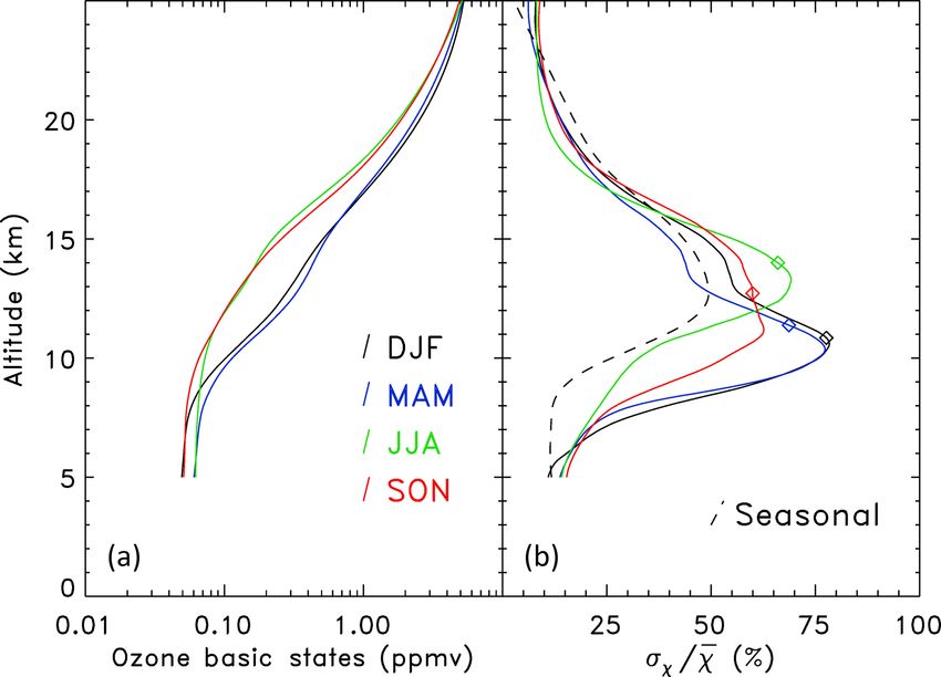
K. Minschwaner et al.: Detection and classification of laminae in balloon-borne ozonesonde profiles                                  1855

                                                                        10 ppbv in the troposphere and 40 ppbv in the stratosphere,
                                                                        which more closely follows our 10 % threshold than the par-
                                                                        tial pressure criteria discussed above.
                                                                           Reid and Vaughan (1991) and Huang et al. (2015) com-
                                                                        pared their methods to “filter and difference” techniques that
                                                                        are broadly similar to the approach used here and in other
                                                                        studies (e.g., Grant et al., 1998; Krizan and Lastovicka, 2005;
                                                                        Thompson et al., 2007a) and found reasonable agreement in
                                                                        lamina statistics between the two methods. One advantage of
                                                                        the filter and difference approach is that basic states are gen-
                                                                        erated for each profile, as described below, which can provide
                                                                        important information on the contribution of laminae to the
                                                                        overall variability in ozone.
                                                                           An important drawback to filtering, however, is directly
                                                                        tied to sharp changes in the vertical gradients of ozone and
Figure 1. Vertical profiles of ozone (a, solid blue) and potential      potential temperature near the tropopause. Figure 2 shows
temperature (b, solid red) measured from Boulder, CO on 10 June
                                                                        observed χ and 2 profiles along with two sets of basic
2008. The respective basic states are indicated by solid black curves
                                                                        state profiles, (χs1 , 2s1 ) and (χs2 , 2s2 ). The first set of ba-
in both panels. Panel (c) shows relative anomalies based on differ-
ences between the measured and basic state profiles for ozone (solid    sic states is derived by applying a nonrecursive boxcar fil-
blue) and potential temperature (solid red, scaled by a factor of 5).   ter with a fixed width of 6 km to each observed profile. A
Dashed vertical lines denote the ±10 % threshold in ozone anomaly       fixed-width filter has been employed in a number of previ-
that is used to identify lamina.                                        ous studies (e.g., Teitelbaum et al., 1994), and for a 6 km
                                                                        boxcar the effective low-pass filter cutoff frequency (∼ 90 %
                                                                        level) corresponds to vertical scales of 2–3 km. These basic
approach for deriving the basic state is modified to improve            states are thus smoothed profiles with all features at scales
detection and identification of laminae located within a few            less than ∼ 2.5 km effectively removed (dashed curves in
kilometers of the thermal tropopause.                                   Fig. 2). Subsequent differencing with the observed profiles
   Dobson (1973) and Reid and Vaughan (1991) used a di-                 produces anomaly profiles that emphasize laminar features
rect sampling method to locate extrema in the vertical profile          less than 2.5 km in width. Note that our 0.1 km averaging and
of ozone partial pressure. They defined a lamina as a local             sampling grid for the measurement profiles corresponds to
maximum or minimum in ozone that exceeded 20 nb in peak                 an effective Nyquist cutoff for scales less than 0.2 km; thus,
magnitude, with a full width between 0.2 and 2.0 km (defined            this method for laminae identification is focused on features
with respect to upper and lower “turning points” bracketing             with widths between about 0.2 and 2.5 km. Features that span
the layer). The use of an absolute threshold rather than a rel-         a vertical range larger than about 3 km occupy a significant
ative one to define a lamina was related to their use of ozone          fraction of the density scale height, and are more often re-
partial pressures, as the change in ozone partial pressure be-          lated to large-scale shifts in air masses than to processes typ-
tween the troposphere and stratosphere is much less than                ically associated with the generation of laminae (Reid and
the corresponding change in ozone mixing ratio. However,                Vaughan, 1991). At vertical scales below 0.2 km, however, an
a fixed 20 nb threshold in partial pressure is roughly compa-           important contribution to ozone variability could result from
rable to our 10 % threshold in mixing ratio only in the middle          the presence of very thin laminae. Aircraft measurements
stratosphere, between about 20 and 30 km altitude. In the UT,           of tracer variability have indicated scale-invariant behavior
mean ozone partial pressures are much lower (25–40 nb) and              over a wide range of horizontal scales, ranging from 0.2 to
the same 20 nb threshold will only detect those anomalies               2700 km (Tuck et al., 2004). Although this suggests that ver-
that are larger than 50 %–80 %. With such a reduced sensi-              tical scales below 0.2 km may be important, the variability in
tivity, the number of lamina detections in the UT should be             ozone at horizontal and vertical scales less than 0.2 km is not
smaller than the number of UT laminae we identify using a               well characterized in the UTLS region.
10 % mixing ratio threshold. Krizan and Lastovicka (2005)                  The method of fixed-width filtering consistently produces
and Krizan et al. (2015) used an even larger threshold of               an apparent lamina of negative sign near the tropopause level
40 nb in peak magnitude to examine “strong” ozone laminae               (Fig. 2). In this case, the effective O3 and 2 perturbations are
in vertical profiles. Alternatively, Huang et al. (2015) used           always less than basic state values due to sharp changes in
a continuous wavelet transform (CWT) approach to study                  the vertical gradients of both quantities near the tropopause.
ozone laminae in lidar ozone vertical profiles. An interesting          Rapid gradient changes near the tropopause usually occur on
feature of the CWT approach is that it does not use a basic             scales less than 2.5 km and therefore are smoothed out in a
state or reference ozone profile to identify laminae. The lam-          basic state derived from a 6 km wide filter. A similar effect
inae amplitude thresholds used by Huang et al. (2015) were              was noted by Schmidt et al. (2008) in their analysis of gravity

www.atmos-chem-phys.net/19/1853/2019/                                                     Atmos. Chem. Phys., 19, 1853–1865, 2019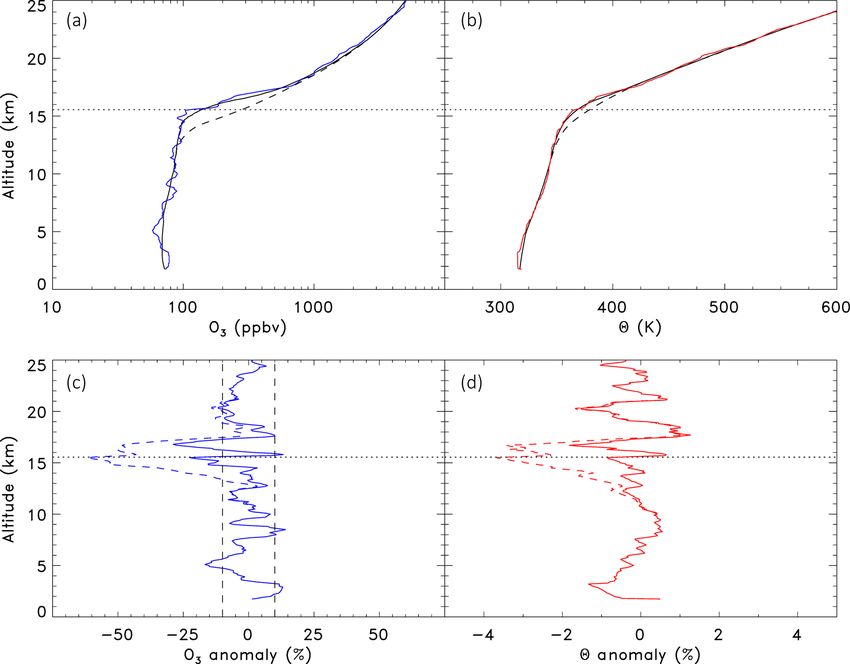
1856                   K. Minschwaner et al.: Detection and classification of laminae in balloon-borne ozonesonde profiles

                                                                          addition, soundings that contain multiple tropopauses (e.g.,
                                                                          Schwartz et al., 2015) are often associated with complex ver-
                                                                          tical structures in ozone that may not be fully characterized
                                                                          by this laminae analysis.
                                                                             The same variable-width smoothing procedure is used to
                                                                          identify laminae in the measured vertical profile of 2. A lam-
                                                                          ina detected in potential temperature that is coincident with a
                                                                          lamina in ozone provides evidence that the sampled air par-
                                                                          cel was subjected to a vertical displacement associated with
                                                                          gravity wave (GW) activity. This method has been used ex-
                                                                          tensively to examine GW signatures in ozonesonde data (e.g.,
                                                                          Teitelbaum et al., 1994; Pierce and Grant, 1998; Thompson
                                                                          et al., 2007a) and in aircraft measurements of ozone (e.g.,
                                                                          Alexander and Pfister, 1995), based on the expectation that

                                                                                      ∂2s ∂χs
                                                                          20 = χ 0        /      ,                                    (1)
                                                                                       ∂z ∂z
Figure 2. Vertical profiles of ozone (a, solid blue) and potential
temperature (b, solid red) measured from Boulder, CO, on 6 Au-            where z is altitude. Teitelbaum et al. (1996) discuss the gen-
gust 2008. Both panels also show basic states calculated using a          eral conditions under which this relationship holds, including
fixed-width filter (dashed) and a variable-width filter (solid), as de-   the condition that the timescales for ozone photochemistry
scribed in the text. The bottom two panels show anomalies based on        are much longer than the timescales relevant for transport by
the fixed-width (dashed) and variable-width (solid) filters for ozone     GW phenomena. They further note that these coincidences
(c, blue), and potential temperature (d, red). Vertical dashed lines      are more readily identified by scaling potential temperature
for the ozone anomaly indicate the ±10 % threshold for laminae            perturbations to account for differences in the mean vertical
detection, and the horizontal dotted lines in all panels indicate the
                                                                          gradients of 2 and χ,
height of the lapse rate tropopause determined from this sounding.

                                                                                     1 dχs         1 d2s
                                                                          R (z) =             /            .                         (2)
                                                                                     χs dz       2s dz
wave activity using GPS temperature profiles. We explored
several alternatives for deriving basic states and minimizing             A similar scaling was employed by Ehhalt et al. (1983)
tropopause-related artifacts, ranging from piecewise polyno-              to compare equivalent vertical displacements obtained from
mial fitting to the use of climatological means. An impor-                measured variances in long-lived stratospheric gases.
tant drawback for many approaches is that they cannot ac-                     One of the most straightforward approaches for identify-
commodate the large degree of variability in the altitude of              ing coincidences in ozone and potential temperature laminae
the tropopause; even seasonal climatologies do not reproduce              involves the spatial correlation between vertical profiles of
tropopause variability to the extent needed to remove false               χ 0 /χs and R20 /2s over a limited vertical domain, for exam-
laminae detections. We adopted a method for RIO SOL that                  ple, within 5 km wide sampling windows (e.g., Teitelbaum et
identifies the primary tropopause for each profile using the              al., 1994). Figure 3 shows a set of relative anomaly profiles
World Meteorological Organization (WMO) lapse rate crite-                 along with the magnitude of the correlation coefficient com-
rion (e.g., Homeyer et al., 2010), and then employs a variable            puted within a 5 km wide vertical window centered at the
boxcar with a maximum width of 6 km and a minimum width                   given altitude. A correlation threshold of r > 0.7 has been
of 1.5 km at the tropopause level. The width varies linearly              shown to be a reliable indicator for GW-induced laminae in
with altitude within 6 km on either side of the tropopause,               ozone (e.g., Pierce and Grant, 1998). One complication with
such that the boxcar width is symmetric about the tropopause              this approach arises when multiple laminae appear within the
level. As shown in Fig. 2, this variable-width filtering method           same correlation window. For example, in Fig. 3 the central
allows the basic states to track sharp gradient changes at the            altitudes of laminae labeled 2 through 5 are close enough to
tropopause while still filtering enough small-scale variability           cause interference in gauging the true correlation within in-
to identify ozone laminae in the anomaly profiles. The use of             dividual laminae. We adopted a different approach for RIO
a variable-width-smoothed basic state means that the detec-               SOL, by correlating over the extent of the laminar feature
tion sensitivity for laminae of varying thickness will change             (where the amplitude exceeds 10 %) or over a 2 km window,
with altitude. Away from the tropopause where the filter-                 whichever is larger. Sensitivity experiments indicate that our
ing width is 6 km, all lamina with vertical scales less than              approach for deriving basic states and for correlating over
∼ 2.5 km can be identified. Near the tropopause, however,                 more limited vertical domains is more consistent with previ-
the mean boxcar width is about 2.6 km, which corresponds                  ous analyses if we adopt a threshold of r ≥ 0.65. In Fig. 3,
to a lamina detection threshold width of about 1.5 km. In                 RIO SOL detects GW ozone lamina (labeled 1 and 3) near

Atmos. Chem. Phys., 19, 1853–1865, 2019                                                    www.atmos-chem-phys.net/19/1853/2019/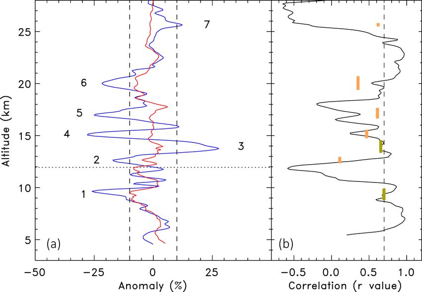
K. Minschwaner et al.: Detection and classification of laminae in balloon-borne ozonesonde profiles                                      1857

Figure 3. Panel (a) shows vertical profiles of ozone (blue) and
scaled potential temperature anomalies (red) from a Boulder            Figure 4. Two simulated ozone profiles with randomly placed lami-
ozonesonde sounding on 4 May 2006. Vertical dashed lines rep-          nae applied to a tropical basic state (a, b), and to a midlatitude basic
resent a 10 % amplitude threshold for defining laminae, and seven      state (c, d). In each case, panels (a) and (c) show the simulated
identified laminae are indicated by number. Panel (b) shows the cor-   ozone (solid) and the derived basic state (dashed), while panels (b)
relation coefficient calculated between ozone and potential temper-    and (d) show the actual anomaly profile for each simulation (solid),
ature anomalies using a 5 km wide sliding vertical window (solid       along with the derived anomaly profile (dashed). Horizontal dotted
curve), and alternatively from windows centered on individual lam-     lines in panels (a) and (c) denote the tropopause level, and vertical
inae (orange and green bars). The dashed vertical line indicates the   dotted lines in panels (b) and (d) denote the 10 % anomaly threshold
0.7 threshold used for identifying gravity wave ozone laminae with     used for detecting ozone laminae.
the 5 km sliding window technique. For correlations over individual
laminae, a 0.65 threshold value is adopted, and laminae meeting or
exceeding this threshold are indicated by the green bars and classi-   enough to produce pairs or triplets of laminae in the derived
fied as GW laminae, while correlations below 0.65 are indicated by     perturbation profile. This effect can be seen in Fig. 4 by the
orange bars and classified as NGW laminae.                             appearance of a false positive lamina near 17 km, which is
                                                                       an artifact produced by the large negative laminae immedi-
                                                                       ately above it. False lamina detections accounted for nearly
9.5 and 14 km altitude with the application of the r ≥ 0.65            25 % of the total number of laminae identified in the sim-
threshold. Laminae for which ozone anomalies are not signif-           ulations, with no altitude dependence in the number of false
icantly correlated with scaled potential temperature anoma-            detections. This is in contrast to the fixed 6 km width smooth-
lies (r < 0.65) are classified as non-gravity wave (NGW)               ing method described in Sect. 3, which generates false lam-
laminae, as there is no evidence that the generation mech-             inae detections at the tropopause in nearly every profile. As
anism is associated with GW activity.                                  expected, the proportion of false detections grows to nearly
   In order to examine the detection sensitivity for laminae,          50 % as the lamina amplitude threshold is reduced from 10 %
we constructed a set of 150 simulated ozone and tempera-               to 5 %. It should be noted that the overall false detection
ture profiles using climatological values representing tropi-          rate is a direct consequence of how these simulations are
cal, midlatitude summer, and midlatitude winter means (An-             designed. Most false detections are associated with a sin-
derson et al., 1986) and introduced localized ozone perturba-          gle large amplitude lamina in the simulation. Although we
tions at random altitudes and over a random sample of am-              expect that the true number of false detections in observed
plitudes and widths. The perturbations were either triangular          ozone profiles is likely smaller, this effect is impossible to
or Gaussian in shape. The simulated profiles were then an-             quantify because there is no way to directly observe the ba-
alyzed using RIO SOL. Figure 4 shows two examples from                 sic state.
the simulations and analysis. In the first example, three lam-            In terms of positive identification of true features, the de-
inae were introduced to a tropical basic state and RIO SOL             tection rate was 79 % for all simulated laminae with ampli-
accurately characterized the anomalies (Fig. 4a and b). The            tudes larger than 10 % and widths between 0.2 and 2.5 km.
amplitudes, widths, and central altitudes of positive and neg-         The detected fraction was degraded to about 60 % for those
ative laminae are derived to within a few percent.                     laminae within ±2 km of the tropopause, primarily because
   The second example is taken from a midlatitude simula-              of the reduced filtering width used to derive the basic states
tion and highlights one of the weaknesses of the filter and            near the tropopause. At all other altitudes, roughly half of the
difference approach. A large amplitude lamina (e.g., near              non-detections arose from simulations involving two or more
18.5 km in Fig. 4c and d) can shift the derived basic state            laminae occurring in close proximity (within a few kilome-

www.atmos-chem-phys.net/19/1853/2019/                                                     Atmos. Chem. Phys., 19, 1853–1865, 2019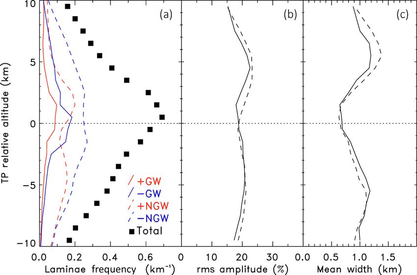
1858                 K. Minschwaner et al.: Detection and classification of laminae in balloon-borne ozonesonde profiles

ters’ altitude) which were counted as a single lamina in the
identification process. Most of the remaining non-detections
were due to simulated laminae with amplitudes just above
the 10 % threshold that were not counted because the derived
amplitudes for these laminae fell just below 10 %. On aver-
age, there is a 2 %–4 % low bias in derived amplitudes using
our version of the filter and difference method, and there is
a tendency to underestimate widths by 0.1 to 0.2 km com-
pared to the simulated inputs. Both of these small biases can
be seen in some of the simulated laminae shown in Fig. 4,
and they are an inevitable result of low-pass filtering to de-
termine the basic state. Laminae altitudes are, however, ac-
curately identified to within ±0.1 km.
   One factor that may introduce a systematic offset to
laminae central altitudes is the finite response time of the      Figure 5. Vertical profiles of ozone laminae characteristics in alti-
ozonesonde. Sonde ascent rates are consistently 4–6 m s−1         tude coordinates relative to the WMO tropopause. Panel (a) shows
and response timescales are ∼ 25 s, leading to a possible         laminae frequency as the number of laminae detected per sound-
systematic bias of between +100 and +150 m in altitude.           ing within 1 km wide altitude bins. Black squares are for all lami-
Note that the offset is unlikely to be any bigger than this be-   nae types and signs. Solid lines show frequencies of GW laminae,
cause we consistently find gravity wave laminae for which         dashed lines indicate NGW laminae, and red and blue colors indi-
the ozone and 2 perturbations (which are based on temper-         cate positive and negative anomalies, respectively. Panels (b) and
ature with response times on the order of a few seconds) are      (c) show profiles of rms amplitudes and mean widths, respectively.
                                                                  The rms amplitudes are derived from the square of the mean rel-
very well correlated on a 100 m grid, with no systematic alti-
                                                                  ative anomaly within each lamina and averaged over all laminae
tude offsets. Given the 1 Hz sampling for the raw data, the ef-
                                                                  detected within corresponding relative altitude bins. Widths are de-
fect of variations in ascent rate which can act to smooth mea-    fined as the full altitude range in which the anomaly amplitude ex-
sured profiles or to limit the resolving of laminar features,     ceeds 10 % (along consecutive 100 m sampling intervals), with a
with scales greater than 0.2 km, is minimal. There are also       minimum restriction of 0.2 km. As with panel (a), solid and dashed
rare, but documented (e.g., Morris et al., 2010), measure-        curves denote GW and NGW laminae, respectively.
ment artifacts that could be mistakenly identified as ozone
laminae. In the case of SO2 interference observed by Mor-
ris et al. (2010), RIO SOL would interpret apparent ozone         tropopause. Our simulations (discussed above) strongly sug-
“notches” as negative NGW ozone laminae.                          gest that this is not an artifact caused by the tropopause, as
                                                                  the false detection rate for simulated ozone laminae was in-
                                                                  dependent of altitude.
4     Results                                                        Figure 5 also displays occurrence frequencies for GW and
                                                                  NGW laminae, segregated by positive (+GW, +NGW) or
4.1    Overall statistics for ozone laminae                       negative anomalies (−GW, −NGW) with respect to the ba-
                                                                  sic states. The most common lamina type is −NGW, which
The RIO SOL analysis was applied to 1138 ozone soundings          accounts for nearly half of all laminae detected outside of
from Boulder, Colorado. As discussed in Sect. 2, these were       the tropopause region. Within 2 km of the tropopause, higher
obtained on a ∼ weekly basis between the years 1991 and           frequencies of +GW and −GW lamina contribute a more
2015. A total of 9952 ozone laminae were identified, cor-         significant amount to the total. Over all altitudes, 28 % of all
responding to a mean number of 8.7 laminae per sounding.          laminae are the GW type and 72 % are NGW laminae. Neg-
The variability in the number of lamina per sounding was          ative anomaly laminae outnumber positive anomaly laminae
very close to a normal distribution about the mean, with a        at most levels, and overall we detect about 15 % more nega-
standard deviation of 2.3 laminae. There were no soundings        tive anomaly laminae.
with fewer than 2 or with more than 16 laminae detections.           Two of the most important characteristics of a laminar
   There are considerable differences in the frequency of         structure are its amplitude and thickness (or width). Figure 5
lamina detections with respect to altitude, season, and lam-      includes panels for the vertical distributions of the root mean
ina type. The number of laminae observations per sound-           square (rms) amplitudes and widths of detected lamina. For
ing within 1 km thick altitude bins relative to the WMO           both rms amplitudes and widths, no significant differences
tropopause is shown in Fig. 5. The occurrence frequency           were found between positive and negative anomaly laminae.
for all ozone laminae maximizes near the tropopause and is        The amplitude of a lamina is defined by the mean of the per-
roughly evenly distributed above and below the tropopause.        turbation taken over the full altitude range in which the per-
Over 60 % of all laminae were observed within 5 km of the         turbation magnitude exceeds the 10 % minimum threshold.

Atmos. Chem. Phys., 19, 1853–1865, 2019                                              www.atmos-chem-phys.net/19/1853/2019/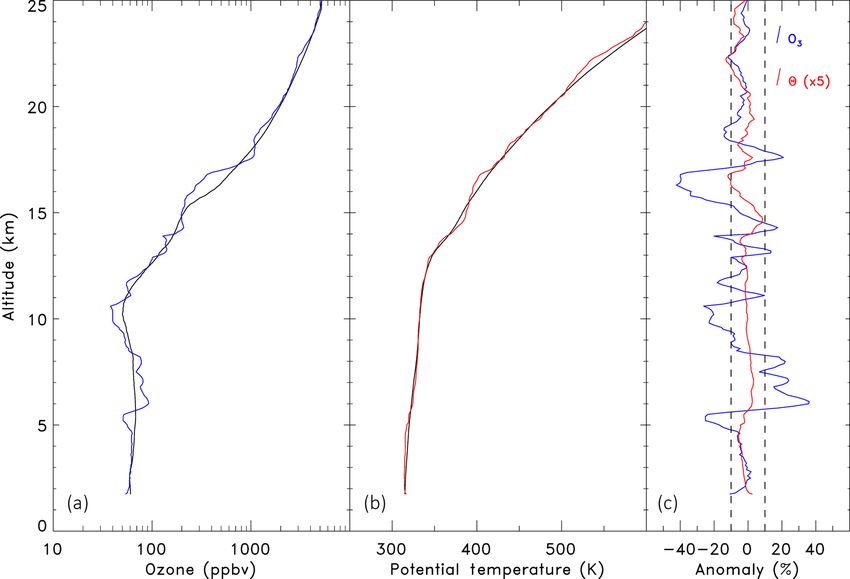
K. Minschwaner et al.: Detection and classification of laminae in balloon-borne ozonesonde profiles                                1859

Figure 5 shows that rms amplitudes are closely matched be-
tween GW and NGW laminae, with values between 15 % and
20 % in the troposphere and an overall tendency for larger
amplitudes in the LS. The mean rms amplitude taken over all
altitudes and laminae type is 20 %. The amplitude distribu-
tion is skewed by the presence of larger-amplitude (> 40 %)
laminae that are seen in ∼ 2 % of the soundings. These large-
amplitude laminae are most often observed in the LS.
   We define laminae widths by the continuous range of alti-
tude levels over which the 10 % minimum amplitude thresh-
old is met in the anomaly profile. Figure 5 shows that av-
erage widths for laminae at Boulder are about 1 km in the
troposphere, decreasing to ∼ 0.7 km near the tropopause and
increasing again in the stratosphere (as noted below, a large
fraction of this variation is a result of the detection method).
The largest mean widths (∼ 1.4 km) were found for NGW
laminae occurring about 5 km above the tropopause. As with         Figure 6. Probability density function (PDF) of the amplitude dis-
amplitudes, no significant differences were found between          tribution for all ozone laminae (a) and contour PDF of width dis-
the mean widths of positive and negative anomalies.                tribution for ozone laminae versus altitude relative to the WMO
   The frequency distribution of laminae widths is shown in        tropopause (b). For the amplitudes, the standard 10 % detection
Fig. 6. It varies with relative altitude as expected because of    threshold is indicated by the vertical dashed line and the solid curve
the variation in basic state smoothing parameters with respect     shows the amplitude distribution using this criterion. The dotted
to the tropopause. At relative altitudes larger than ±5 km,        curve shows the extension of the amplitude PDF if a 5 % detection
the distribution has a significant tail in which lamina widths     threshold is employed. For the width PDF, contours are separated
up to 2.5 km are observed. Closer to the tropopause, we find       by 0.02, and the black dashed line indicates the tropopause level.
a truncation of the width distribution around 1.5 km results
from changing the filtering parameters for the basic states.
If we assume that distribution of laminae widths far from          and 10 % shown in Fig. 6 should be regarded as an upper
the tropopause is representative of the entire profile, then       limit on the true occurrence of small-amplitude laminae.
we can estimate that roughly 16 % of ozone laminae near               The above statistics for Boulder may be contrasted with
the tropopause may not be identified because their widths          those obtained using previous methodologies, namely the use
are larger than our upper detection limit in this region. This     of a fixed width, 6 km boxcar filter for the basic state and
undetected fraction estimated from Fig. 6 is consistent with       a 5 km wide correlation window for O3 and 2 anomalies.
the laminae simulations discussed above, in which the frac-        For this particular method, the total number of laminae de-
tion of undetected laminae increased by 19 % within 2 km of        tected is 25 % smaller and their mean widths are more than
the tropopause. It should be noted, however, that the simu-        twice as large as those from RIO SOL shown in Fig. 5, rang-
lated negative lamina at 18 km in Fig. 4 is within 1.2 km of       ing from 1 km up to a maximum of 3 km at the tropopause.
the tropical tropopause, and it is accurately characterized by     These differences can be attributed to the dominating influ-
RIO SOL. On the narrow side of the width distribution, ex-         ence of tropopause-induced laminae for the case of a fixed-
trapolation of the smoothly decreasing widths below modal          width boxcar. The apparent tropopause lamina appears in
values of ∼ 0.4 km at all altitudes yields a detection loss rate   over half of the soundings and it is sufficiently wide to mask
of about 2 %–4 % due to lamina with widths narrower than           or absorb any other individual laminae that may be present
0.2 km.                                                            within 2–3 km of the tropopause. Not surprisingly, we also
   Figure 6 also shows the frequency distribution of laminae       detect fewer overall positive laminae when using the fixed-
amplitudes. Note that the distribution is truncated at 10 % by     width boxcar. There are also changes to the relative fraction
the minimum threshold used for lamina detection. Sensitivity       of GW and NGW laminae when using a 5 km wide correla-
runs using smaller minimum thresholds indicate a significant       tion window; relatively more GW laminae are detected and
number of small (5 %–10 % amplitude) laminae fall below            this fraction maximizes at the tropopause level in association
our 10 % minimum, as indicated in Fig. 6. A mean of about          with the aforementioned spurious tropopause-induced lami-
12 laminae are detected per sounding using a 5 % minimum           nae in both O3 and 2.
amplitude threshold, an increase of about 40 % laminae over           A preliminary analysis has also been done using RIO SOL
using a 10 % threshold. As discussed above, the fraction of        in its standard configuration for other measurement sites at
false detections grows with decreasing amplitude threshold,        midlatitude and low-latitude stations, and the results appear
so that the frequency estimate for amplitudes between 5 %          to be similar in accuracy to those from Boulder. At Pago
                                                                   Pago, Samoa, we find comparable statistics with a slightly

www.atmos-chem-phys.net/19/1853/2019/                                                Atmos. Chem. Phys., 19, 1853–1865, 2019
1860 K. Minschwaner et al.: Detection and classification of laminae in balloon-borne ozonesonde profiles
higher overall frequency of laminae (nearly 10 per profile), a
30 % GW fraction, and a similar altitude distribution relative
to the tropopause. On the other hand, when applying RIO
SOL to winter–spring soundings in and around the Antarctic
polar vortex or during particular cold periods in the Arctic
winter, the criteria and thresholds for both ozone laminae and
the tropopause would likely require significant changes in or-
der to maintain a robust analysis, especially under conditions
of significant ozone depletion and/or changes to the thermal
structure of the lower stratosphere. A detailed comparison of
ozone laminae from different measurement sites is planned
for future investigations, but in this paper, our emphasis is
on a description of techniques and on the climatology from
Boulder.
4.2 Basic states and ozone variance
Figure 7. Seasonal means of ozone basic states profiles from Boul-
der over the years 1991–2015 (a) and normalized standard devia-
As discussed in Sect. 3, the filter and difference approach tions of the basic states (b). The means and intra-seasonal standard
produces basic state profiles that can be used to quantify the deviations were taken over the periods December–February (DJF,
fraction of overall variability in ozone attributable to lami- black), March–May (MAM, blue), June–August (JJA, green), and
nar features in the profile. Figure 7 shows the climatologi- September–November (SON, red). The standard deviations were
cal means and standard deviations of basic states for each of normalized by mean values at each altitude, and seasonal mean
the four seasons (December–January–February is denoted by tropopause heights are indicated by colored triangles. Also shown
DJF, etc.). These are displayed in altitude coordinates rather is comparable magnitude of the seasonal variation in basic states
than tropopause-relative coordinates in order to highlight (dashed curve, b), estimated from the variance in the four seasonal
seasonal differences. Because of the filtering methods used to basic states and normalized by the annual mean. Note that this sea-
√
sonal magnitude is equivalent to Ap / 2 for a cosine seasonal vari-
derive these basic states, all of the basic state variability in the
ation, where Ap is the peak relative amplitude.
UT arises from ozone changes occurring on vertical scales
larger than 2–3 km. The mean basic states are nearly identi-
cal to climatological seasonal means obtained from the raw decomposed into these components, then
data, so that many of the expected seasonal effects are seen in
the mean basic state profiles. For example, larger ozone mix- (σT /χ )2 = (A)2 + (σs /χ )2 + (δ)2 , (3)
ing ratios occur during winter and spring in the 10 to 20 km
altitude range as a result of stratospheric transport and sea- where A is the rms amplitude of detected laminae, σs2 is the
sonal changes in the tropopause height. This seasonality can variance in the basic state profile, and δ is the normalized
be quantified by the standard deviation of the seasonal basic variance due to small-amplitude (< 10 %) features. The left
states at each altitude, as shown in Fig. 7, and can be directly side and the two largest terms on the right side of Eq. (3) are
compared with the intra-seasonal (i.e., within each season) shown in Fig. 8 for the seasons of DJF and JJA. Raw ozone
variability derived from the standard deviation of each of the data were used to calculate σT2 , while (A)2 and σs2 were de-
seasonal mean profiles. As noted above, the seasonal com- rived from the laminae amplitudes and basic state outputs of
ponent of ozone variability is largest between 12 and 16 km the RIO SOL analysis. Figure 8 shows that the total vari-
altitude. However, the intra-seasonal basic state variability ance in ozone is generally controlled by large vertical-scale
tends to follow the climatological tropopause and maximizes changes near and immediately below the tropopause. Lam-
in the UT about 1–2 km below the WMO tropopause. Dur- inae make up an important fraction of the total variance,
ing winter and spring, there is a secondary increase in LS however, and these features can be the dominant mode of
variability (12–15 km), which is likely to be related to deep ozone variability in the middle troposphere and lower strato-
stratospheric intrusions of tropical/subtropical air like those spheric regions. The contribution from small-amplitude fea-
investigated by Reid et al. (2000). tures (δ)2 was calculated from the results of the threshold
In summary, we expect contributions to the total intra- sensitivity experiments discussed above (or could also be es-
seasonal ozone variance arising from three types of features: timated as a residual from Eq. 3), and this contribution is
(i) detected laminae with widths between 0.2 and 2.5 km typically between 0 % and 5 % of the total variance. Figure 8
and amplitudes greater than 10 %, (ii) all variations with also shows seasonal and altitude means of the contributions
larger vertical scales (> 2.5 km), and (iii) small-amplitude from all three terms on the right side of Eq. (3), indicated
(< 10 %) features across all vertical scales. Assuming that within boundaries of a coordinate system defined by the am-
the total intra-seasonal ozone variance σT2 can be effectively plitude and the vertical scale of ozone variations. Our results
Atmos. Chem. Phys., 19, 1853–1865, 2019 www.atmos-chem-phys.net/19/1853/2019/K. Minschwaner et al.: Detection and classification of laminae in balloon-borne ozonesonde profiles 1861
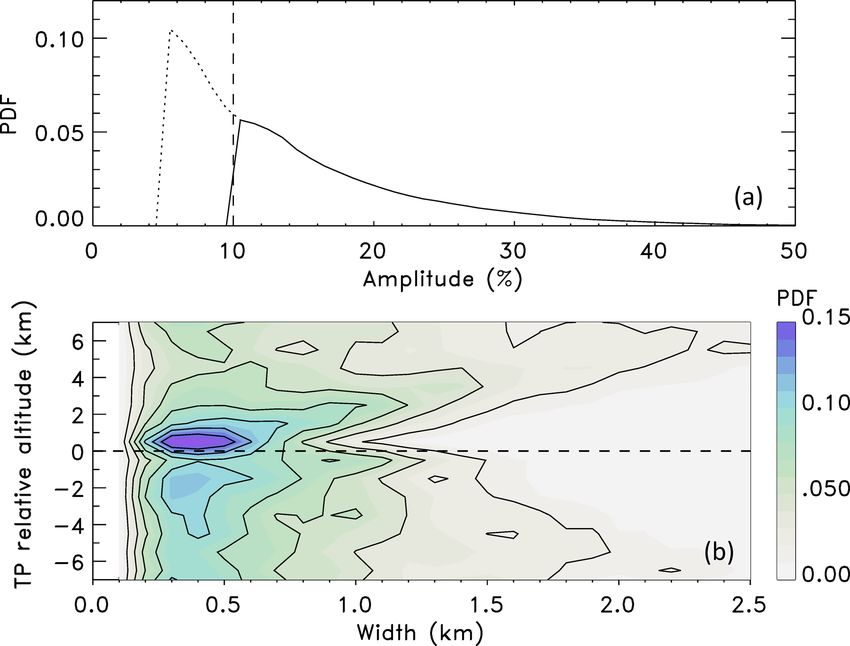
Figure 9. Climatology of ozone laminae frequency at Boulder, CO,
as a function of month and altitude relative to the WMO tropopause
for GW (a) and NGW (b) laminae. Frequency is expressed as the
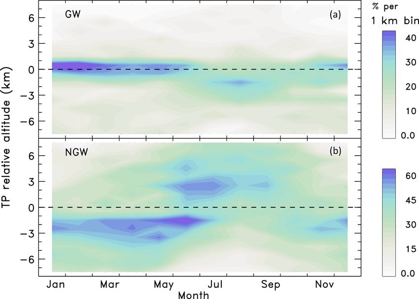
Figure 8. Normalized seasonal variances in ozone for DJF (a) and percent of soundings that contain one or more GW or NGW lam-
JJA (b). Plotted are the normalized total variance (solid gray), basic inae within 1 km altitude bins relative to the tropopause. Note the
state variance (dotted), laminae variance (solid black), and the sum different scales between GW and NGW frequencies.
of basic state and laminae variances (dashed). Panel (c) shows the
annual mean contributions to the total variance between 5 and 25 km
altitude, as a function of amplitude and the vertical scale of features
in the ozonesonde profile. example, our simulations suggest that GW laminae are more
readily detected and identified as such in regions where back-
ground vertical gradients of ozone and potential temperature
indicate that, on average, more than half of the intra-seasonal are both large, such as in the LS region.
variance in ozone between 5 and 25 km altitude is due to The distribution of NGW laminae stands in stark contrast
large-scale changes in the basic state, and that slightly over to that of GW laminae, and, as noted in the Introduction, the
one-third of ozone variations are due to laminar features that generating mechanisms for NGW laminae are much more
are identified by RIO SOL. uncertain. Previous analyses have used maximum correlation
threshold criteria between ozone and potential temperature to
4.3 Boulder laminae climatology infer the influence of Rossby waves on ozone (e.g., Pierce
and Grant, 1998; Thompson et al., 2007a). We have not
We examine here how the frequency of detected laminae adopted this approach in RIO SOL due to larger uncertain-
varies with altitude and season. Figure 9 shows monthly ties in positively classifying these laminae using ozone and
mean frequencies relative to the WMO tropopause for potential temperature alone, particularly since the connection
GW and for NGW ozone laminae. Consistent with Fig. 5, between O3 and 2 is not as clear as indicated in Eq. (1) for
GW laminae are most often observed within 2 km of the GW ozone laminae. However, it is plausible that a significant
tropopause, whereas NGW laminae are more evenly dis- fraction of NGW laminae are generated in processes associ-
tributed throughout the UTLS. Throughout most of the year, ated with Rossby wave activity. The seasonality of Rossby
the GW frequency distribution maximizes slightly above the wave breaking (RWB) in the UTLS at northern midlatitudes
tropopause, while the NGW frequency is larger below the (e.g., Hitchman and Huesmann, 2007; Isotta et al., 2008) is
tropopause. This situation reverses during the months of similar to the seasonality of UT NGW ozone laminae seen in
June–September, when more GW laminae are detected be- Fig. 9. Rossby wave breaking and stratosphere–troposphere
low the tropopause and most NGW laminae are found above exchange (STE) are both prevalent along the flanks of UT
the tropopause. jets (Gettelman et al., 2011 and references therein), and stud-
Climatologies of gravity wave momentum fluxes indicate ies of jets using meteorological reanalysis data show a maxi-
a wintertime maximum in the LS for this location (e.g., mum in subtropical UT jet frequencies near 30◦ latitude from
Geller et al., 2013). However, it should be noted that while November through April in the Northern Hemisphere (Man-
our ozone GW laminae climatology is expected to be related ney et al., 2011, 2014). An associated phenomenon of multi-
to the overall level of gravity wave activity, there are other ple tropopause events, which are often linked to tropopause
factors that can influence whether a GW lamina in ozone is folds and extratropical STE (e.g., Sprenger et al., 2003), also
generated at the location of an ozonesonde profile in the first shows maximum frequencies during December–March on
place, and then whether it will be detected by RIO SOL. For the northern flank of the subtropical jet maximum (e.g., Man-
www.atmos-chem-phys.net/19/1853/2019/ Atmos. Chem. Phys., 19, 1853–1865, 20191862 K. Minschwaner et al.: Detection and classification of laminae in balloon-borne ozonesonde profiles
ney et al., 2014), and these events are responsible for a sig- still significantly less than the number of laminae detected at
nificant fraction of the variability in ozone and other trace Boulder. The method used by Huang et al. (2015) limited the
gases in the tropopause region (Schwartz et al., 2015). smallest scale of detected laminae to 0.5 km as compared to
Mechanisms leading to the maximum in NGW laminae the 0.2 km limit used here; thus, it is likely that the differ-
frequency in the LS during summer are more uncertain. Jing ence can largely be explained by the detection of laminae at
and Banerjee (2018) found a maximum in anticyclonic RWB smaller scales and with smaller amplitudes (due to the use of
on the 350 and 370 K 2 surfaces during NH summer, and a relative amplitude threshold in RIO SOL). The root-mean-
both of these surfaces are typically at or above the tropopause square laminae amplitude at Boulder is about 20 % relative
level over Boulder during summer. In addition, they showed to the basic state. This mean amplitude does not vary sig-
that the zonal distribution of summer RWB favored those nificantly with altitude. It is slightly larger than the ∼ 15 %
regions above and immediately upstream of Boulder. How- mean amplitude determined by Pierce and Grant (1998) for
ever, the production of laminar features in summertime LS ozonesondes from Wallops Island, Virginia, although their
ozone from other mechanisms cannot be ignored. Impacts identification method could have been impacted by interfer-
on the composition of the midlatitude summer LS have been ence near the tropopause. The mean width of ozone laminae,
demonstrated from monsoon-related dynamics (e.g., Randel defined by the altitude range in which the anomaly amplitude
et al., 2010), deep summertime convection (e.g., Weinstock exceeds 10 %, varies between 0.7 and 1.4 km depending on
et al., 2007), and meridional transport from the tropical UT the altitude relative to the tropopause and is generally small-
(e.g., Bönisch et al., 2009). Clearly, more work is needed est near the tropopause. Some of the variation in mean width
to understand the full range of dynamical and chemical pro- with altitude is a result of the filtering procedure used in RIO
cesses that may produce the range of laminar ozone features SOL.
seen in these balloon profiles and in other ozone measure- Laminae statistics have been examined on a tropopause-
ments. The development of methods to further classify NGW relative altitude grid rather than on standard altitudes rela-
laminae and to associate mechanisms with their generation is tive to the surface. This gridding better delineates the subset
a focus of ongoing work using RIO SOL. of laminae generated by primarily tropospheric mechanisms
from those resulting from mainly stratospheric phenomena
and facilitates the identification of STE processes. The oc-
5 Conclusions currence frequency for ozone laminae shows a distinct maxi-
mum within ∼ 2 km of the tropopause and is nearly symmet-
We have described the RIO SOL analysis package for charac- ric above and below the tropopause. GW laminae make up
terizing ozone laminae in balloon soundings and presented an about one-third of all ozone laminae. These are most often
analysis of the ∼ 25-year ozonesonde dataset from Boulder, detected near the tropopause in the lower stratosphere. NGW
Colorado. RIO SOL involves an adaptation of the filter and laminae are more abundant, and negative NGW are the most
difference approach used in previous studies of ozonesonde dominant laminar feature throughout the UTLS region.
profiles, in which a unique basic state is generated for each The total variance in the Boulder ozonesonde dataset was
ozone profile and laminae are identified as deviations from decomposed into terms representing changes in the ozone ba-
this basic state. The major improvements in RIO SOL in- sic state, changes due to the presence of ozone laminae, and
clude methods for improved sensitivity in identifying GW changes due to weaker-amplitude (< 10 %) features. Large-
laminae using potential temperature from each sounding and scale changes in the basic state account for 60 % of the to-
for avoiding false detections of GW laminae near the thermal tal intra-seasonal ozone variance. The magnitudes of intra-
tropopause. The vertical gridding of the ozonesonde data and seasonal variations in basic states are comparable to those
the filtering method constrain the range of vertical scales for of the seasonal cycle. Laminae detected by RIO SOL are re-
identified laminae to between 0.2 and 2.5 km. Simulations in- sponsible for 37 % of the total variance in ozone, and the
dicate that RIO SOL can reliably identify most of the ozone remaining 3 % is estimated to originate from smaller-scale
laminae with relative amplitudes greater than 10 %, and vir- features. Although they are not the dominant form of ozone
tually all laminae above 20 % amplitude. variability, laminae must be considered in order to quantify
The mean number of ozone laminae observed per sound- ozone variability and trends in the UTLS region. Future re-
ing at Boulder is about nine. This is much higher than the search in this area should be directed towards methods for
number (one–two) reported by Reid and Vaughan (1991) and obtaining global laminae datasets, either from satellite mea-
Krizan et al. (2015) from analyses of northern midlatitude surements or from ozonesonde networks, and towards the de-
soundings, but as noted in the Introduction, the fixed detec- velopment of improved techniques for unambiguous identi-
tion threshold used in these studies emphasized stratospheric fication of the mechanisms responsible for generating NGW
ozone laminae at the expense of tropospheric laminae. Huang ozone laminae.
et al. (2015) used separate thresholds for the troposphere and
the stratosphere and found a mean of 2.5 laminae per profile
in the ozonesonde dataset from Huntsville, Alabama. This is
Atmos. Chem. Phys., 19, 1853–1865, 2019 www.atmos-chem-phys.net/19/1853/2019/K. Minschwaner et al.: Detection and classification of laminae in balloon-borne ozonesonde profiles 1863
Code and data availability. NOAA ozonesonde datasets may be ozonesondes from different manufacturers, and with differ-
accessed from the data archive maintained by the Ozone and Wa- ent cathode solution strengths: The Balloon Experiment on
ter Vapor Group at the NOAA Earth System Research Labora- Standards for Ozonesondes, J. Geophys. Res., 113, D04307,
tory, Global Monitoring Division, at https://www.esrl.noaa.gov/ https://doi.org/10.1029/2007JD008975, 2008.
gmd/ozwv/ozsondes/ (Johnson et al., 2018). The RIO SOL analy- Deshler, T., Stübi, R., Schmidlin, F. J., Mercer, J. L., Smit, H. G.
sis package is written in Interactive Data Language (IDL) program- J., Johnson, B. J., Kivi, R., and Nardi, B.: Methods to homoge-
ming code and is available upon request by contacting the lead au- nize electrochemical concentration cell (ECC) ozonesonde mea-
thor. surements across changes in sensing solution concentration or
ozonesonde manufacturer, Atmos. Meas. Tech., 10, 2021–2043,
https://doi.org/10.5194/amt-10-2021-2017, 2017.
Author contributions. KM led the writing and analysis for the Dobson, G. M. B.: The laminated structure of ozone in the atmo-
manuscript with significant contributions from GLM and IP and sphere, Q. J. Roy. Meteor. Soc., 99, 599–607, 1973.
comments from all authors. ATG and AFJ developed major com- Dütsch, H. A.: Two Years of Regular Ozone Soundings Over Boul-
ponents of the RIO SOL analysis package in consultation with all der, Colorado, NCAR Tech Note 01, National Center for Atmo-
authors. IP, BJJ, and AFJ provided ozonesonde data and advised on spheric Research, Boulder, CO, USA, 1966.
their use with RIO SOL. Ehhalt, D. H., Röth, E. P., and Schmidt, U.: On the temporal vari-
ance of stratospheric trace gas concentrations, J. Atrnos. Chern.
1, 27–71, 1983.
Competing interests. The authors declare that they have no conflict Fairlie, T. D., Avery, M. A., Pierce, R. B., Al-Saadi, J., Dibb,
of interest. J., and Sachse, G.: Impact of multiscale dynamical processes
and mixing on the chemical composition of the upper tropo-
sphere and lower stratosphere during the Intercontinental Chemi-
cal Transport Experiment–North America, J. Geophys. Res., 112,
Acknowledgements. Partial support was provided by a subcontract
D16S90, https://doi.org/10.1029/2006JD007923, 2007.
to New Mexico Tech from the Microwave Limb Sounder group
Geller, M. A., Alexander, M. J., Love, P. T., Bacmeister, J., Ern, M.,
at the Jet Propulsion Laboratory, for undergraduate student re-
Hertzog, A., Manzini, E., Preusse, P., Sato, K., Scaife, A. A., and
search in atmospheric physics. Kenneth Minschwaner is grateful
Zhou, T.: A comparison between gravity wave momentum fluxes
to Anne Thompson for valuable advice on ozonesonde flight
in observations and climate models, J. Climate, 26, 6383–6405,
operations, data analysis, and the study of ozone laminae.
2013.
Gettelman, A., Hoor, P., Pan, L. L., Randel, W. J., Heg-
Edited by: Andreas Hofzumahaus
glin, M. I., and Birner, T.: The extratropical upper tropo-
Reviewed by: three anonymous referees
sphere and lower stratosphere, Rev. Geophys., 49, RG3003,
https://doi.org/10.1029/2011RG000355, 2011.
Grant, W. B., Pierce, R. B., Oltmans, S. J., and Browell, E. V.:
Seasonal evolution of total and gravity wave induced laminae
References in ozonesonde data in the tropics and subtropics, Geophys. Res.
Lett., 25, 1863–1866, 1998.
Alexander, M. J. and Pfister, L.: Gravity wave momentum flux in Hassler, B., Petropavlovskikh, I., Staehelin, J., August, T., Bhartia,
the lower stratosphere over convection, Geophys. Res. Lett., 22, P. K., Clerbaux, C., Degenstein, D., Mazière, M. D., Dinelli, B.
2029–2032, https://doi.org/10.1029/95GL01984, 1995. M., Dudhia, A., Dufour, G., Frith, S. M., Froidevaux, L., Godin-
Anderson, G. P., Clough, S. A., Kneizys, F. X., Chetwynd, J. H., Beekmann, S., Granville, J., Harris, N. R. P., Hoppel, K., Hubert,
and Shettle, E. P.: AFGL atmospheric constituent profiles (0– D., Kasai, Y., Kurylo, M. J., Kyrölä, E., Lambert, J.-C., Levelt,
120 km), Rep. AFGL-TR-86-0110, 43 pp., Air Force Geophys. P. F., McElroy, C. T., McPeters, R. D., Munro, R., Nakajima,
Lab., Hanscom AFB, Mass., USA, 1986. H., Parrish, A., Raspollini, P., Remsberg, E. E., Rosenlof, K. H.,
Appenzeller, C. and Holton, J. R.: Tracer lamination in the strato- Rozanov, A., Sano, T., Sasano, Y., Shiotani, M., Smit, H. G. J.,
sphere: A global climatology, J. Geophys. Res., 102, 13555– Stiller, G., Tamminen, J., Tarasick, D. W., Urban, J., van der A,
13569, 1997. R. J., Veefkind, J. P., Vigouroux, C., von Clarmann, T., von Sav-
Bönisch, H., Engel, A., Curtius, J., Birner, Th., and Hoor, P.: Quanti- igny, C., Walker, K. A., Weber, M., Wild, J., and Zawodny, J.
fying transport into the lowermost stratosphere using simultane- M.: Past changes in the vertical distribution of ozone – Part 1:
ous in-situ measurements of SF6 and CO2 , Atmos. Chem. Phys., Measurement techniques, uncertainties and availability, Atmos.
9, 5905–5919, https://doi.org/10.5194/acp-9-5905-2009, 2009. Meas. Tech., 7, 1395–1427, https://doi.org/10.5194/amt-7-1395-
Bowman, K. P., Pan, L. L., Campos, T., and Gao, R.: Observa- 2014, 2014.
tions of fine-scale transport structure in the upper troposphere Hitchman, M. H. and Huesmann, A. S.: A seasonal climatology of
from the High-performance Instrumented Airborne Platform Rossby wave breaking in the 320–2000-K layer, J. Atmos. Sci.,
for Environmental Research, J. Geophys. Res., 112, D18111, 64, 1922–1940, 2007.
https://doi.org/10.1029/2007JD008685, 2007. Homeyer, C. R., Bowman, K. P., and Pan, L. L.: Extrat-
Deshler, T., Mercer, J. L., Smit, H. G. J., Stubi, R., Levrat, ropical tropopause transition layer characteristics from high-
G., Johnson, B. J., Oltmans, S. J., Kivi, R., Thompson, A. resolution sounding data, J. Geophys. Res., 115, D13108,
M., Witte, J., Davies, J., Schmidlin, F. J., Brothers, G., and https://doi.org/10.1029/2009JD013664, 2010.
Sasaki, T.: Atmospheric comparison of electrochemical cell
www.atmos-chem-phys.net/19/1853/2019/ Atmos. Chem. Phys., 19, 1853–1865, 2019You can also read