Scalable photonic-based nulling interferometry with the dispersed multi-baseline GLINT instrument - Caltech Authors
←
→
Page content transcription
If your browser does not render page correctly, please read the page content below
ARTICLE
                  https://doi.org/10.1038/s41467-021-22769-x                 OPEN

                  Scalable photonic-based nulling interferometry
                  with the dispersed multi-baseline GLINT
                  instrument
                  Marc-Antoine Martinod 1,2,3 ✉, Barnaby Norris 1,2,3, Peter Tuthill1,2,3, Tiphaine Lagadec 4,
                  Nemanja Jovanovic5, Nick Cvetojevic 6, Simon Gross7, Alexander Arriola7, Thomas Gretzinger                                                7,

                  Michael J. Withford7, Olivier Guyon8,9,10,11, Julien Lozi8, Sébastien Vievard8,10, Vincent Deo8,
1234567890():,;

                  Jon S. Lawrence12 & Sergio Leon-Saval 1,2,13

                  Characterisation of exoplanets is key to understanding their formation, composition and
                  potential for life. Nulling interferometry, combined with extreme adaptive optics, is among the
                  most promising techniques to advance this goal. We present an integrated-optic nuller whose
                  design is directly scalable to future science-ready interferometric nullers: the Guided-Light
                  Interferometric Nulling Technology, deployed at the Subaru Telescope. It combines four
                  beams and delivers spatial and spectral information. We demonstrate the capability of the
                  instrument, achieving a null depth better than 10−3 with a precision of 10−4 for all baselines,
                  in laboratory conditions with simulated seeing applied. On sky, the instrument delivered
                  angular diameter measurements of stars that were 2.5 times smaller than the diffraction limit
                  of the telescope. These successes pave the way for future design enhancements: scaling to
                  more baselines, improved photonic component and handling low-order atmospheric aber-
                  ration within the instrument, all of which will contribute to enhance sensitivity and precision.

                  1 Sydney Institute for Astronomy, School of Physics, The University of Sydney, Sydney, NSW, Australia. 2 Sydney Astrophotonic Instrumentation Laboratories,

                  Physics Road, University of Sydney, Sydney, NSW, Australia. 3 AAO-USyd, School of Physics, University of Sydney, Sydney, NSW, Australia. 4 Research
                  School of Astronomy and Astrophysics, Australian National University, Canberra, ACT, Australia. 5 California Institute of Technology, Pasadena, CA, USA.
                  6 Laboratoire Lagrange, Observatoire de la Côte d’Azur, Université Côte d’Azur, Nice, France. 7 MQ Photonics Research Centre, Macquarie University,

                  Sydney, Australia. 8 Subaru Telescope, National Astronomical Observatory of Japan, National Institutes of Natural Sciences, Hilo, HI, USA. 9 Steward
                  Observatory, University of Arizona, Tucson, AZ, USA. 10 Astrobiology Center, National Institutes of Natural Sciences, Mitaka, Tokyo, Japan. 11 James C.
                  Wyant College of Optical Sciences, University of Arizona, Tucson, AZ, USA. 12 Australian Astronomical Optics - Macquarie, Macquarie University, Sydney,
                  NSW, Australia. 13 Institute of Photonics and Optical Science, School of Physics, University of Sydney, Sydney, NSW, Australia. ✉email: marc-antoine.
                  martinod@sydney.edu.au

                  NATURE COMMUNICATIONS | (2021)12:2465 | https://doi.org/10.1038/s41467-021-22769-x | www.nature.com/naturecommunications                                 1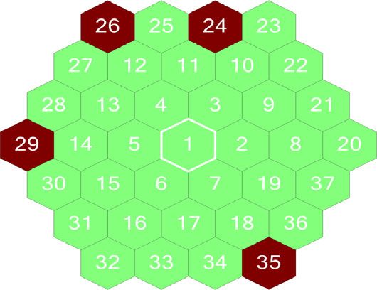
ARTICLE                                                                  NATURE COMMUNICATIONS | https://doi.org/10.1038/s41467-021-22769-x

W
             ith more than 4300 exoplanets confirmed so far1,                  null depth, defined as the ratio of the intensity of destructive over
             questions of the characterisation of their chemistry             constructive interference, which quantifies the degree of sup-
             and physical conditions have become pressing. Indir-             pression of the light due to spatial brightness distribution of the
ect detection methods, such as transit or precision radial velocity           source. It is recovered by the processing of the measured null
observations, have revealed the ubiquity and the diversity of                 depth, but biased by the instrumental response and seeing-
exoplanetary systems. However, few Earth-analogue exoplanets                  induced effects. The precision of its measurement is affected by
orbiting in the habitable zone of their host star have been dis-              fluctuations arising from various sources, including atmospheric
covered and present challenges for either technique. Direct ima-              seeing, vibrations, detector noise, etc. This precision can be
ging is one of the methods under development to study such                    improved using statistical data-analysis and fitting methods such
systems, not only able to provide orbital parameters but also                 as described here.
characterise the surface, the atmosphere, the weather and even                   Several conceptual improvements for space-based observa-
probe for signatures of life2–4. However, many observational                  tories have been proposed for imaging15 and high angular
challenges remain.                                                            resolution capabilities16. Theoretical studies into instrumental
   In order to observe and study planets located in the habitable             effects on the nulled light such as spectral dispersion and
zone, it is critical to suppress the overwhelming glare from direct           polarisation have also been made17. Several ground-based
starlight over scales of angular resolution much smaller than one             nullers have been built, including the BracewelL Infrared Nul-
arcsecond5. The contrast ratio between the faint speck of plane-              ling Cryostat18, the Keck Interferometric Nuller (KIN)19, the
tary light and the star ranges between ~10−4 for massive, self-               Palomar Fiber Nuller (PFN)20 and the Large Binocular Tele-
luminous hot exoplanets observed in the mid-infrared6, to 10−10               scope Interferometer Nuller (LBTI)21. In addition to their
for Earth-like exoplanets imaged in reflected light from their host            technological innovation, these instruments produced a range
star7. An exoplanet in the habitable zone (~1 AU) around a star               of important scientific results. For example, KIN, which com-
in a nearby star-forming region (~100 pc) has an angular                      bined both 10 m Keck Telescopes, performed a major survey of
separation from its host star of 10 milliarcseconds (mas here-                exozodiacal dust around 47 nearby stars, using 10 spectral
after). Such systems lie somewhat beyond the diffraction limit of             channels ranging from 8 μm to 13 μm wavelengths (N band)22.
8–10 m class telescopes (40 mas at 1.55 microns on an 8-m                     More recently, the LBTI has investigated the presence of dust
aperture and 32 mas on a 10-m aperture), and within range of                  closer to the habitable zone of nearby stars as part of the
next-generation large apertures. However, atmospheric turbu-                  HOSTS survey23, also in N band, critical for future exo-Earth
lence blurs the images and limits the uncorrected resolving power             imaging endeavours. While these instruments relied on con-
to about one arcsecond, hence the need for adaptive optics sys-               ventional bulk-optical components, the Palomar Fiber Nuller
tems to reach the diffraction limit of the telescope.                         used the spatial filtering properties of optical fibres to improve
   Coronagraphy, combined with adaptive optics, is the most                   the instrumental null depth, combining light from two sub-
developed method to address the needs for simultaneous high                   apertures of the 5.1 m Palomar Telescope at Ks band (~2.2 μm).
contrast ratio at high angular resolution. Several major instru-              It also introduced the numerical self-calibration method
ments worldwide such as SPHERE8, GPI9, SCExAO10 and the                       (NSC)24, i.e., the analysis of the statistical fluctuations of the
vortex coronagraphs of Keck11 all deploy various forms of                     measured null depth to deduce the underlying source null
coronagraphs. One performance metric for such devices is the                  depth, yielding sufficient precision to detect a faint companion
inner-working angle (IWA) conventionally defined as the                        in a binary system25 and a component of the disk around AB
spatial separation from the optical axis over which off-axis objects          Aur26.
would have a 50% throughput of the peak throughput of the                        We have built a nulling interferometer, built upon the GLINT
coronagraph. Current generation coronagraphs struggle to reach                (Guided-Light Interferometric Nulling Technology) framework.
IWAs close to the formal diffraction limit: Dλ (where λ is the                Unlike the aforementioned instruments, it performs all opera-
wavelength and D the diameter of the telescope)12. For a modern               tions within a photonic chip. An earlier prototype, (“GLINT
large (~8 m) telescope operating in the near-infrared, this                   South”) deployed at the Anglo-Australian Telescope in Australia,
limit rules out exploration of habitable zone orbits of Sun-like              emphasised study of the performance of the photonic technology
(or cooler) stars for all but a tiny handful of very nearby systems.          itself (refs. 27,28 and Lagadec et al., manuscript in prep.) under
   An alternative method is nulling interferometry13. Drawing                 seeing-limited conditions. The design of previous photonic nul-
upon long baseline interferometry (or aperture masking), beams                lers (like PFN) fundamentally limited the nulling to only be
of starlight from separate telescopes (or sub-apertures) are                  performed on a single baseline. The GLINT instrument is opti-
brought together where they interfere. The distinction is that a              mised for science by taking advantage of wavefront correction
nulling interferometer is configured with a π radian phase shift               provided by the adaptive optics system (AO)29 and by being the
between the beams so that on-axis light will destructively inter-             first photonic instrument capable of nulling multiple baselines
fere. Consequently, the starlight is cancelled out at the centre of           simultaneously, with the delivery of six non-redundant inter-
the image plane and often redirected into a separate path. The                ferometric baselines. Its optical circuitry yields dedicated outputs
light coming from an off-axis source carries a phase-shift                    for the destructive interference, the constructive interference as
imposed by the non-axial angle of incidence so that the condi-                well as a simultaneous photometric monitor for each beam, all
tion for destructive interference is not met and the light is not             reformatted to deliver spectral information by cross-dispersion in
nulled. Such an arrangement means that light coming from a                    a spectrograph. GLINT is integrated into the Subaru Corona-
nearby companion, such as a planet, may be isolated from the                  graphic Extreme Adaptive Optics system (SCExAO)10,30,31, at the
star. Unlike coronagraphs, the effective IWA of nulling inter-                Subaru Telescope.
ferometers (shortened to “nullers”) depends on the baseline                      This use of integrated-optics technology yields a straightfor-
                                               λ 14
B separating the apertures so that IWA ¼ 2B         . Also unlike cor-        ward and scalable approach to combine several apertures—up to
onagraphs, this effective IWA is not a hard limit; rather (as                 spanning the whole pupil for the case of a single large telescope
demonstrated in this paper) spatial structure can continue to be              aperture—delivering significant improvement to sensitivity and
resolved much closer to the star, at the expense of a lower                   imaging capability. The other assets of this technology are spatial
achievable contrast. The primary observable is called the source              filtering, flexibility of design, and straightforward implementation

2                 NATURE COMMUNICATIONS | (2021)12:2465 | https://doi.org/10.1038/s41467-021-22769-x | www.nature.com/naturecommunications
NATURE COMMUNICATIONS | https://doi.org/10.1038/s41467-021-22769-x ARTICLE
a) SCExAO system Subaru facility Object b) 3 4
AO188
Adapve opcs (low-order Telescope
system correcon)
GLINT
1
IMR MEMS Shuer
MASK
Prism V-groove MLA POLA
Detector
Photonic chip 2
Opcal fibres PUPIL
CAM
IMG
CAM
Fig. 1 Global schematic of GLINT and configuration of the apertures of the mask. a Global schematic of GLINT and its integration within the Subaru
Telescope and SCExAO. Within GLINT itself the sequence of optical systems encountered consists of the image rotator (IMR), a pupil mask, a steerable
segmented mirror (MEMS), a shutter and a linear polarising beamsplitter (POLA). The science beam is then injected by a microlens array (MLA) into the
photonic chip while the dichroic beamsplitter delivers light to cameras viewing both the image plane and pupil plane. The processed beams coming from
the photonic chip are spectrally dispersed in the GLINT spectrograph then imaged on the science detector (C-Red 2). b Diagram of the segmented MEMS
mirror with highlighted segments in red matching the pattern of holes in the mask. Segments 29, 35, 26 and 24 are identified with beams 1, 2, 3 and 4,
respectively. The lengths of baselines range from 2.15 m (combination of the beams 3 and 4) to 6.45 m (combination of the beams 2 and 3).
of complex optical processing such as GLINT’s spectroscopic the pupil plane. Each segment can be individually moved in tip
back-end. We therefore incorporate all the main characteristics of and tilt to maximise the injection of the light into the waveguides
previous-generation nullers, while adding the features enabled by in the chip, and in piston to scan the phase of the interferometer
integrated-optics (most notably multiple, simultaneously nulled arms hence the fringes and adjust the position of the dark fringe.
baselines), in a single device. Next, a polariser selects a single linear polarisation state and a
GLINT aims to demonstrate the design of a highly capable, dichroic beamsplitter divides the beams between the science
scalable instrument for future large telescopes, such as the channel and alignment-camera channel. Transmitted beams are
Extremely Large Telescope (ELT) or Thirty-Metre Telescope injected into the photonic chip by way of a microlens array. The
(TMT), and for long baseline interferometers like the Very Large beam reflected by the beamsplitter is sent to a two-camera system
Telescope Interferometer (VLTI). Furthermore, the use of pho- used for metrology and alignment that is capable of viewing both
tonic chips facilitates the realisation of advanced architectures the image and pupil planes. The image-viewing camera allows
such as the multi-tier combiner16 or kernel-nulling32,33 aiming setting the point-spread-function (PSF) position such that the
for robust performance against time-varying instrumental phase. beam is aligned with the optical axis of the chip. The pupil-
In this work, we show that the combination of integrated- viewing camera is used to align the MEMS mirror segments with
optics technology with more advanced data analysis algorithms the holes in the mask as well as with SCExAO’s telescope pupil
(built upon the numerical self-calibration method) improves the mask (which has spiders), all of which appear superimposed.
precision of the nulling data, with enhanced performance against Taken together, these viewing systems enable alignment and
both random and systematic errors. The achieved null depth monitoring of GLINT’s internal optics, together with registration
is better than 10−3 with a precision of 10−4 for all baselines, with with respect to SCExAO and Subaru.
λ/8 RMS simulated seeing applied. On-sky commissioning The core element of GLINT is the integrated-photonic chip
demonstrates the performance of GLINT in real condition with (for more detailed technical information, see ‘Specifications of the
the successful determination of the angular diameters of two stars instrument’ in “Methods”) which performs all the primary
that are 2.5 times smaller than the diffraction limit of the interferometric operations on the starlight. The chip consists of
telescope. two parts. The first one is a pupil remapper (Fig. 2a) which has
four inputs, each fed by a sub-aperture of the primary mirror. It
coherently reformats the 2-dimensional array of the beams into a
Results one-dimensional configuration suitable for feeding the second
Description of the instrument. GLINT’s underlying optical part. This is the beam combiner section (Fig. 2b–d) which
design has been described in a previous article29 and for con- interferometrically combines each pair of beams and provides
venience is briefly set out here. The Subaru Telescope’s 8-m monitoring of the injection efficiency. The chip delivers 16 output
mirror collects light and firstly routes it to the AO-188 adaptive beams: four photometric taps, six outputs carrying the destructive
optics facility34 for low-order wavefront correction. Starlight next interference of all six pairs of beams (baselines), identified as null
traverses the SCExAO extreme AO system where it receives high outputs, and six with the constructive interference from the same
order correction. The beam is finally redirected toward the pairs, identified as anti-null outputs. These outputs are individu-
GLINT optical table (Fig. 1a) with the first element being an ally redirected into the GLINT spectrograph, located in a stable
image rotator to control the angle of projection of the baselines place elsewhere on the Nasmyth platform via 16 separate optical
onto the sky plane. The telescope pupil is re-imaged onto an fibres inserted into a single protected cable. Finally, the spectrally
opaque carbon fibre mask, containing four apertures that provide dispersed beams are projected on a C-Red2 InGaAs camera35
six non-redundant baselines (Fig. 1b). The pupil is undersized to withARTICLE NATURE COMMUNICATIONS | https://doi.org/10.1038/s41467-021-22769-x
b)
Coupler
0.3
Z axis [mm]
Splitter
0.25
80
Beam 3
Beam 4 Beam 2 60
0.2 Beam 1 ]
m
-6.5 -6 -5.5
40 [m
-5 -4.5 is
-4 ax
X axis [mm] Y
c) 80 d) 0.3
70 0.28
Y axis [mm]
Z axis [mm]
60 0.26
50 0.24
40 Coupler 0.22
Inputs Outputs
Splitter
0.2
-6.5 -6 -5.5 -5 -4.5 -4 30 40 50 60 70 80
X axis [mm] Y axis [mm]
Fig. 2 Schematics of the integrated-optics chip. a Schematics of the pupil remapper of the chip, coherently transforming the 2D configuration of the inputs
(on the left) matching the desired pupil sampling pattern into a 1D configuration (on the right). The waveguide paths have been optimised to match their
optical path lengths despite their different routes. The green waveguide is associated with beam 1, orange with beam 2, red with beam 3 and blue with
beam 4. b Perspective view of the beam combiner of the chip. c Plan view in which light propagates from the 4 inputs at the bottom towards the top,
encountering 4-way splitters and codirectional couplers. d Right-side view of the chip showing the locations of the inputs and the outputs. The inputs,
outputs, splitters and couplers are indicated on the (b–d) diagrams. The axis scale proportions in all the schematics differ for clarity in the drawing.
observation. Therefore, the optical propagation lengths of the from small variations in intensity of the writing-laser) would
waveguides and the characteristics of the splitters and couplers manifest as refractive index variations along the waveguide.
were studied. Alternatively (or possibly in addition to), mismatched optical
The first phase of characterisation included the measurement paths external to the chip might arise in the alignment of the
of optical path length differences between all pairs of waveguides. microlens array with respect to the chip. As will be described, the
It was performed by scanning the phase of each baseline (by effects of the OPD mismatch for 4 baselines is presently managed
incrementally pistoning the associated MEMS segment) while the by accounting for the instrumental loss of coherence in the data
null-channel output intensities (integrated over a 200 nm analysis model, and performing measurements on some baselines
bandwidth) were recorded. The position of the centre of the sequentially. Improvements in the ULI manufacturing process,
fringe envelope was then recovered by fitting with a simple model including more comprehensive parameter scans and real-time
(a more comprehensive multi-wavelength model is detailed in the monitoring of waveguide OPD during fabrication, will address
subsection “Data processing”). The intensity I as a function of these issues in future chip iterations.
delay δ is given by: The second phase of characterisation focused on the coupling
! coefficients of the codirectional couplers and the splitting
2π δ δ0 coefficients of the splitters within the chip. The recovered null
IðδÞ ¼ A þ B sin ðδ δ 0 Þ þ ϕ sinc Δλ : ð1Þ
λ0 λ20 depth depends on both the coherence of the light and on any
variations in flux between the incoming beams. The latter may
where A and B are respectively the incoherent term and the arise as rapidly fluctuating phenomena (e.g., scintillation and
amplitude of the fringe pattern, λ0 is the wavelength at which the variations of injection) or on longer timescales (e.g., instrumental
scan is performed and Δλ the bandwidth, δ0 is the parameter of transmission along differing paths). Measurement of the
interest: the optical path difference (OPD) between the two beams instantaneous fluxes of all input beams, simultaneous with the
at the centre of the envelope. λ0 and Δλ were known and the other interference measurements, avoids inaccuracy arising due to
parameters were fitted to the data. time-varying fluxes (e.g. from fast wavefront errors coupling to
It is seen on Fig. 3 that, for this optical alignment, only two injection losses). This represents a more robust solution for flux
baselines, N1 and N4, exhibit data that span the centre of the fluctuations compared to non-simultaneous beam-chopping
fringe envelopes. To reach the central null the other baselines based methods implemented by previous generation nulling
require an OPD offset that exceeds the mechanical piston range interferometers19–21.
of the MEMS segmented mirror. Furthermore, the optical path Detailed knowledge of all splitting and coupling ratios
lengths are different between all waveguides. Although some level delivered by devices inscribed within the chip was needed to
of mismatch is inevitable, it is important to identify and perform an unbiased correction of the photometric contribution
subsequently improve the on-chip cophasing in future chip to the null depth. The coefficients of the four splitters and the six
fabrication rounds. couplers of the chip were measured as a function of wavelength
The most likely cause for the inconsistent optical delays is using the supercontinuum source of the SCExAO bench. The
physical differences in the optical paths through the system for splitting coefficient is defined by
the 4 input beams, either internal or external to the chip itself. Ix
Within the remapper or the coupler sections of the chip, non- Sx ¼ ; ð2Þ
uniformity in the waveguide engraving process (for example, Ip þ Ia þ Ib þ Ic
4 NATURE COMMUNICATIONS | (2021)12:2465 | https://doi.org/10.1038/s41467-021-22769-x | www.nature.com/naturecommunicationsNATURE COMMUNICATIONS | https://doi.org/10.1038/s41467-021-22769-x ARTICLE Fig. 3 Scanned fringe envelopes for each of the six baselines. Subplots (a to f) respectively represent the baselines N1 to N6 scanned over the full available range of the optical path difference (OPD) from data taken in July 2019 with illumination from the supercontinuum source within SCExAO. The blue dots are the data and the orange curve is the fitted model. The label of the horizontal axis “OPDx−y” shows the segment of the beam x was scanned with respect to the reference beam y. The value in each plot is the fitted δ0. Fig. 4 Splitting, coupling ratios and ζ coefficients of the beam combiner. a Splitting ratios of beam 1 between the photometric output and the three couplers with respect to wavelength. b Coupling ratios of the coupler combining the beams 1 and 2 with respect to wavelength. c ζ coefficients for beams 1 and 2 for the outputs of Null 1 with respect to wavelength. where I is the flux of the output of interest x of the splitter among The coupling coefficient Cn is defined as the fraction of light in p, a, b, c, which are respectively the photometric tap and the three a coupler going to the null output couplers. Figure 4a presents the splitting coefficients for beam In 1 into its 4 components, which are seen to be chromatic over the Cn ¼ ð3Þ full waveband. These plots are representative of all splitters, which I n þ I an produce similar results. where In and Ian are the fluxes in the null and anti-null output, NATURE COMMUNICATIONS | (2021)12:2465 | https://doi.org/10.1038/s41467-021-22769-x | www.nature.com/naturecommunications 5
ARTICLE NATURE COMMUNICATIONS | https://doi.org/10.1038/s41467-021-22769-x
respectively. Similarly to the case for the splitters, Fig. 4b shows
that the coefficients of the coupler combining the beams 1 and 2
are a function of wavelength; again a finding representative of all
couplers on the chip.
Consequently, a scale factor, the ζ-coefficient, was applied to
the flux measured in a photometric tap before using it to correct
the bias in the null depth. This coefficient is defined by
I i±
ζ i± ¼ ð4Þ
I p;i
where I i± is the flux of beam i in the antinull or null output and
Ip,i is the flux of beam i in the photometric output. This coefficient
was measured when only one beam is illuminated (Fig. 4c). These
ζ-coefficients not only took into account the spectral variations of
the splitting and coupling ratios, but also the instrumental
transmission coefficients between the chip and the detector,
ensuring a direct estimation of the contribution of a beam in the
coupler over all wavelengths. Following this analysis, it was
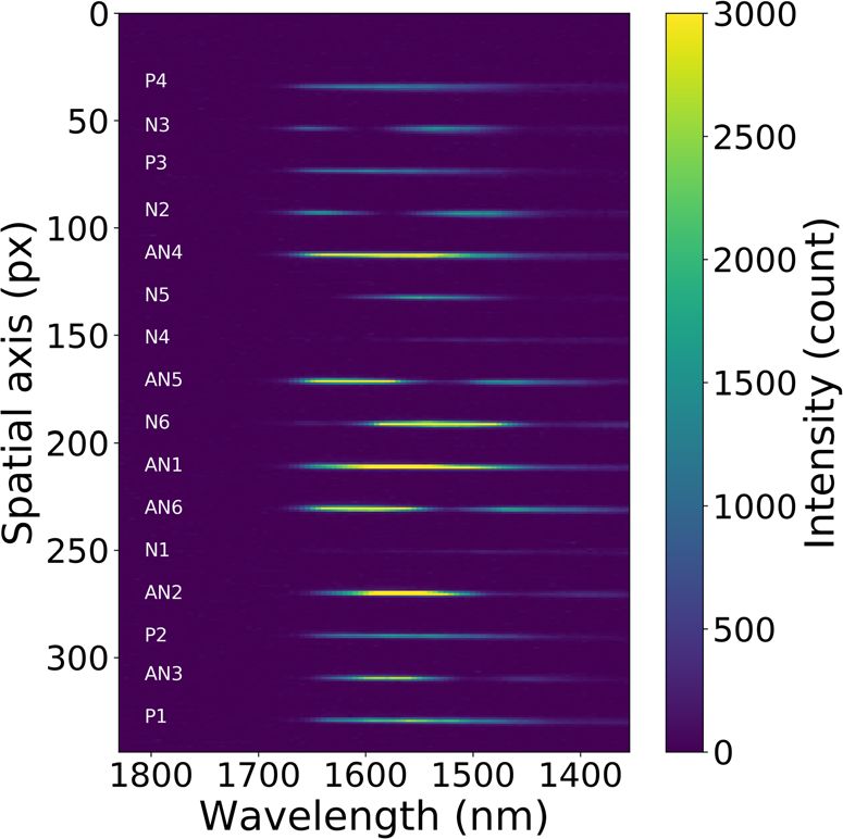
Fig. 5 A data frame from the science sensor illuminated with a laboratory
possible to determine the contribution of any given beam to the
source. Spectral dispersion runs along the horizontal direction, while
null or anti-null signal by using the measurement of flux from the
outputs from different waveguides are displaced in vertical rows. The rows
photometric tap.
labelled “P” are the photometric tap. “N1-6” are the outputs corresponding
to the null output and “AN1-6” are the outputs corresponding to the
Data processing. The data processing relies on the NSC method,
respective anti-null outputs. On this occasion, pistons on the MEMS mirror
which has been adapted to this particular configuration of GLINT
were configured to produce a nulled signal on N1 and N4.
that has multiple baselines, and expanded to encompass spectral
dispersion36. NSC uses measured statistical distributions of the
anti-null outputs were swapped. In order to mitigate the impacts
various seeing-induced and instrumental perturbations along
of these long-tails with poor phase control and recover a
with the measured null depth to determine the underlying source
distribution closer to Gaussian, frames were sorted and those
null depth. This self-calibration reduces or removes the reliance
with high phase variation removed by a sigma-clipping filter. This
on observations of calibrator stars. It has been shown that
filter operated by keeping frames for which the fluxes in the null
operation over large bandwidths introduces a bias that limits the
(anti-null) output lie within two standard deviations from the
attainable null depth17. In spectrally dispersing the light, GLINT
smallest (largest) value. Frames falling outside sigma-clipping
observes narrow bands, minimising any bias and effectively
limits for either null or anti-null outputs were discarded from the
approaching monochromatic performance. Spectrally dispersing
analysis.
light also yields new information, both astrophysical and instru-
The data processing consisted of two steps: (i) measuring the
mental. Fluctuations in injection and phase variations are key to
photometry, detector noise, the null depths and determining their
the measurement of the source null depth but are affected by
probability density function (PDF) using histograms after
chromaticity. Biases for both can be more accurately compen-
applying the sigma-clipping, and (ii) fitting a model PDF—which
sated with wavelength-diverse information. Consequently, spec-
is a function of the source null depth—to the observed PDF of the
tral dispersion reduces bias on null depth measurements and
null depth.
improves precision over non-dispersed detection, as illustrated
The flux of a spectral channel (defined by the width of a pixel)
with on-sky data in the following sections. Astrophysical
at wavelength λ was measured by summing the flux along the
exploitation of the spectral diversity of null depths is also possible,
spatial axis over the width of each output (Fig. 5). This operation
but not yet done. Whereas fluctuations of injection were directly
was done for every spectral channel of the 16 outputs, for every
measured in each spectral channel and used in the data proces-
remaining frame. The same procedure was performed on dark
sing, the version of GLINT discussed here was not able to mea-
frames.
sure the instantaneous phase of the fringes. Thus, the fluctuations
Next, data was processed for the baseline of interest over the
of phases were assumed not to be wavelength-dependent to first
desired spectral bandwidth. For each of its spectral channels at
order; an approximation that had been tested and validated with
wavelength λ, the histograms of the photometric outputs of the
the results in the following sections. Recovery of instantaneous
data were calculated. The same operation was done for the
fringe phase is planned for the next instrument upgrade, however
detector noise in the interferometric outputs of the dark frames.
even just correcting for chromatic injection, spectral dispersion
The null depth, defined as the ratio of the flux of the null
delivers enhanced null depth measurements with less systematic
output divided by the flux in the anti-null, was calculated for each
error compared to broadband light.
spectral channel for all remaining data frames. The uncertainty at
It was assumed that the variations of OPD were normally
each point in the null depth histogram was derived from the
distributed in the statistical analysis. Although the true distribu-
number of elements in each bin i and follows a binomial
tion was unknown, this assumption was reasonable as the AO
distribution:
system ensured that phase variations remain smaller than 2π,
preventing drift or phase wrapping of the fringes during the f obs;λ ðiÞð1 f obs;λ ðiÞÞ
acquisition. However, various atmospheric issues, uncorrected by σ 2obs;λ ¼ ; ð5Þ
the AO, could skew the phase variations away from a normal M null;λ
distribution, such as the island effect37 which consists of sharp
phase discontinuities across the telescope’s spiders mainly where σobs,λ(i) is the uncertainty of the normalised histogram fobs,
exacerbated by thermal effects when the ground wind speed is λ(i) for the i-th bin at the wavelength λ, and Mnull,λ is the number
low. The variations could be as high as π radians, so the null and of data frames measured for this wavelength.
6 NATURE COMMUNICATIONS | (2021)12:2465 | https://doi.org/10.1038/s41467-021-22769-x | www.nature.com/naturecommunicationsNATURE COMMUNICATIONS | https://doi.org/10.1038/s41467-021-22769-x ARTICLE
average seeing during the night of the 20th of June 2020 ranged
between 0.3 and 0.5 arcseconds at 1600 nm, but with some
significant wavefront error resulting from low-wind-effect and
telescope vibrations. Data were acquired for 15 min at a frame
rate of 1400 Hz for the pairs of baselines N1, N4 and N5, N6. The
null depth was measured for all baselines on a spectrally dispersed
signal from 1525 to 1575 nm. An illustrative example of model
fitting to the histograms of the null depth of the baseline N1 on α
Boo is given in Fig. 7.
δ Vir is also a red giant branch star, with a magnitude in H
band of −1.05 mag and a measured angular diameter of 10.6 ±
Fig. 6 Source null depth with respect to baseline by observing the 0.736 mas in H band39, i.e., around 20% of the diffraction limit.
supercontinuum source of the SCExAO bench. The blue dots represent the The conditions of observation for the night of the 5th of July
null depths measured from the binned spectral channel while the orange 2020, and the configuration of the acquisition were the same as
dots represent the null depths measured with spectrally dispersed light. for α Bootis, detailed above.
Once the null depths were obtained for the four baselines, the
The model of the PDF was generated for each spectral channel angular diameter of α Bootis was deduced from the fitting of these
from the known distributions of the intensities and detector four null depths by a model that gave the expected null leakage
noise, and from the unknown quantities that are the source null given the stellar size, here parameterised by a uniform disk
1V diameter:
depth N obj;ij ¼ 1þV obj;ij , the position μOPD and the scale factor σOPD
obj;ij
1 V UD
of the OPD normal distribution; they constituted the three free N UD ¼ ; ð6Þ
parameters to fit (see “Modelling the null depth” in “Methods”). 1 þ V UD
The generation was done with a Monte-Carlo approach because so that
of the presence of large phase errors despite the AO corrections29.
J πθ B
The PDF models were fitted to the observed PDF on all spectral 1 UD λ
V UD ¼ 2 ð7Þ
channels, simultaneously, to obtain the parameters. πθUD Bλ
where J1 is the Bessel function of the first kind, θUD is the angular
Laboratory performance: null depth of an unresolved source. diameter, B the baseline and λ the wavelength.
The aim of this part of the study was to use null depths measured The result of this fit of null depth as a function of the baseline
by GLINT to explore the efficacy of spectral dispersion in nulling. is given in Fig. 8a. The four source null depth points are an
GLINT also enables exploration of the stability of the instru- excellent match to the form of the expected curve and yield
mental null depth between different baselines. parameters within the range of expected literature values. The
The supercontinuum source of SCExAO was used. It provides angular diameter found is 19.7 ± 0.1 mas with a reduced χ2 of
a spatially coherent wavefront so that the theoretically-expected 52.0. The uncertainty has been rescaled by the square root of the
null depth should be zero. Atmospheric turbulence was simulated reduced χ2. The χ2 is high because the error bars are derived only
by applying a moving Kolmogorov phase screen to the SCExAO from statistical diversity in the data and do not account for
deformable mirror, corresponding to a winds peed of 10 m.s−1 systematics (for example blurring due to seeing variations faster
with an RMS wavefront error of 200 nm (~λ/8). The null depth than the frame rate.)
was then calculated in the bandwidth between 1525 and 1575 nm To evaluate the efficacy of spectral dispersion, the stellar
both with and without the spectrally dispersed signal (the latter diameter was also obtained from spectrally binned null depth
obtained by binning the spectral channels). First, the observed data over the same bandwidth. The found diameter is 24.2 ± 1.7
null depths appear to be independent of baseline (Fig. 6), mas, which is systematically larger than the established value
confirming the expected stability of the instrument and spatial (between 19.1 and 20.4 mas). This overestimation of null depth is
coherence of the source. explained by the fact the fringes of the two baselines N5 and N6
Second, the instrumental non-dispersed null is around 3.5 ± could not be set to the central dark fringe (Fig. 3e) causing a
0.31 × 10⁻³ over a bandwidth of 50 nm. The use of spectral systematic loss of coherence. The spectrally dispersed signal
dispersion over the same bandwidth allows us to reach a null allows this to be accounted for in the model resulting in the
depth 3.8 times deeper at 0.92 ± 0.11 × 10⁻³ and with a similar delivery of the expected value of null depths.
improvement in measurement precision. The histograms of the null depths for δ Vir were processed and
This improvement between the dispersed and the non- fitted in the same way. As before, the four source null data points
dispersed null depths and their measurement precision illustrates yield an excellent fit to the model (Fig. 8b), which in turn is in
the influence of the bandwidth on the measurements, and the agreement with literature expectations for this star (expected UD
improvement afforded by the spectrally-dispersed measurement diameter of 10.6 mas). The angular diameter found is 10.9 ± 0.1
and model. Even so, the null depth is not quite zero, which may mas with a reduced χ2 of 11.2 where the uncertainty has been
be due to factors not included in the model such as blurring of the rescaled as before. As for α Boo, the high χ2 betrays the presence
fringes by vibrations faster than the frame rate. of systematic errors not taken into account in the measurement of
the null depth, such as high-frequency phase jitter40. One option
Performance on sky: measurement of two stellar diameters. would be to combine the self-calibration with a standard PSF-
GLINT was deployed on-sky to determine the apparent angular reference star calibration.
diameters of α Bootis and δ Virgo.
α Bootis is a red giant branch star, with magnitude in H band Discussion
of −2.81 mag and with published angular diameter measure- GLINT embodies a new generation of source nulling inter-
ments between 19.1 and 20.4 mas38 in K band. This is around ferometers. It exploits photonic technology to create multiple
40% of the λ/D diffraction limit of the telescope in our band. The interferometer baselines which can be simultaneously nulled.
NATURE COMMUNICATIONS | (2021)12:2465 | https://doi.org/10.1038/s41467-021-22769-x | www.nature.com/naturecommunications 7ARTICLE NATURE COMMUNICATIONS | https://doi.org/10.1038/s41467-021-22769-x Fig. 7 Histograms of the measured null depth of base N1 computed over 10 dispersed spectral channels with the fitted curves. Each subplot from (a) to (j) shows the histogram of the measured null depth of base N1 on α Boo (blue dots) and the fitted model (orange curve), in each of the spectral channel spanning from 1525 to 1570 nm. The fitted parameters are Nobj,12 = 7.05 × 10⁻² ± 1.86 × 10⁻⁴, μOPD = 302 ± 0.465 nm and σOPD = 163 ± 0.163 nm for a reduced χ2 of 2.51. Fig. 8 Variations of the source null depth of α Boo and δ Vir and their respective fitted curves with respect to the baseline. a Variation of the source null depth of α Boo (blue dots) as a function of baseline together with the best-fit model (blue solid curve). The orange area highlights the expected range of null depth at 1550 nm for an expected UD diameter between 19.1 and 20.4 mas (obtained from the literature). Error bars represent the standard error of the measurements. b Source null depth of δ Vir (blue dots) with baseline together with the best-fit model (blue solid curve). The orange gives the expected range of null depth for a UD diameter between 9.86 and 11.3 mas (from the literature). The error bars represent the standard deviation of the fitted value of the source null depth given by the covariance matrix of the fit of the histogram, rescaled by the reduced χ2 of that fit. Active optical elements within the instrument allow delays to be describing the random statistical error contribution. GLINT was finely adjusted, switching different pairs into null operation, or demonstrated on-sky with measurements of the diameters of two even swapping null and anti-null configuration. The instrument stars, both well below the formal λ/D diffraction limit of also boasts multi-channel spectral information by way of a the telescope (the smaller of the two being 5 times less than the spectroscopically dispersed back-end. diffraction limit). The spatial angular scales probed by GLINT are Source null depths measured on the laboratory test-bench with of immediate relevance to direct imaging campaigns targeting a point-like source and a seeing simulator are better than 10−3, exoplanets in the habitable zone around nearby star systems. 3.8 times deeper than that obtained using the non-spectrally- Considered individually, the raw performance metrics of GLINT dispersed method. These measurements also gave results con- are comparable with the best previous-generation nullers, how- sistent with on-sky data, yielding precision of the order of 10−4, ever this instrument shows a pathway in which the 8 NATURE COMMUNICATIONS | (2021)12:2465 | https://doi.org/10.1038/s41467-021-22769-x | www.nature.com/naturecommunications
NATURE COMMUNICATIONS | https://doi.org/10.1038/s41467-021-22769-x                                                                                                                      ARTICLE

                                                                                          R = 160 at 1.55 μm. It consists of an AusOptic 16-channel V-groove glass array
 Table 1 Identification table cross-referencing the nulled and
                                                                                          with a 127 μm pitch and an angled physical-contact (APC) fibre connector, in
 anti-nulled outputs with the corresponding pair of beams                                 which the photonic chip output fibres are set, a collimator with a focal length of
 together with the length of the baseline on sky.                                         65.1 mm then a BK7-glass 1-inch equilateral prism from Altechna. The sixteen
                                                                                          dispersed beams are focused, by a lens of focal length of 150 mm, on the detector.
                                                                                               Photodetection is performed with a C-Red2 InGaAs camera, replacing the
 (Anti-)null                         Pair of beams                    Baseline (m)        photodetectors used in the previous version of GLINT. The total detector area is
 (A)N1                               1-2                              5.55                cropped around the dispersed beams so that the dimensions of the grabbed frames
 (A)N2                               2-3                              6.45                are reduced to 344 × 96 pixels (Fig. 5), allowing a maximum frame rate of 1400 Hz,
 (A)N3                               1-4                              4.65                i.e., an integration time of 0.7 ms. This value is around 7 times faster than the
                                                                                          median atmospheric coherence time of 5.14 ms at Mauna Kea49 so the turbulent
 (A)N4                               3-4                              2.15                phase screen is effectively “frozen” for each frame. The subsequent improvement of
 (A)N5                               3-1                              3.2                 the instrumental null is counterbalanced by a reduction in the final sensitivity due
 (A)N6                               2-4                              5.68                to the read-out noise of the detector at high frame rates. Future evolution of the
                                                                                          instrument plans to use an e-APD camera with better (less than one electron) read-
 The numbering is as adopted in Fig. 1b.                                                  out noise.

straightforward ability to scale photonics technology up to                               Observing procedure. Due to the optical path delay limitations noted in the
                                                                                          subsection “Characterisation of the photonic chip” in “Results”, simultaneous nulls
encompass more beams, more combined baselines and incorpo-                                on four baselines at once were not achievable and so observations were performed
rate spectral diversity both optically and as an integrated aspect of                     by nulling two baselines at a time.
the data reduction. The goal to span the entire telescope pupil,                              The instrument was aligned using the supercontinuum source integrated into
making use of the full light gathering capability of a large tele-                        the SCExAO bench the day before the night of observation. The static aberrations
                                                                                          on the bench were corrected by the deformable mirror to deliver a flat wavefront,
scope, is within reach.                                                                   and an active tip-tilt control loop prevented any drift during the alignment
   These ambitions point the way to future improvements in the                            procedure of GLINT.
design of next-generation photonic chips for nulling inter-                                   The first step consisted of maximising the injection of the light into GLINT by
ferometry. The achromatic performance of the couplers, and the                            moving the tip-tilt positions of the segments of the MEMS. The real-time software
                                                                                          of GLINT automatically performs this operation by mapping and interpolating the
internal and external optical path length matching should both be                         injection with respect to the tip-tilt of the segments.
better controlled to enable straightforward operation of a larger                             The second and last step consisted in finding the appropriate delay to be added
number of simultaneous nulled baselines. This would form a base                           by the MEMS mirror to achieve the deepest null depth for each baseline. Each
for the deployment of photonic nulling interferometers on future                          baseline was scanned by pistoning the appropriate MEMS segment while the total
                                                                                          flux of the null output was monitored, and fitted with a sine function to find the
ELTs or interferometers, such as in the mid-infrared for the                              point corresponding to maximum contrast and to determine the actual OPD of the
VLTI41. Further areas of research include management of wave-                             dark fringe for data processing. The optimal set of values for tip/tilt and piston
front errors, and new architectures capable of recovery of the                            were then stored.
instantaneous baseline phase, while delivering astrophysical data                             Once on-sky, these optimisation scans were repeated with starlight (in a smaller
within the same device. Such improvements would deliver feed-                             domain about the optimum found in the lab, to save time). This accounted for any
                                                                                          mechanical drifts in the instrument between the lab and on-sky measurements,
back to adaptive optics systems tasked with correcting low-order                          different static aberrations and atmospheric angular dispersion. The drift in terms
aberrations, with immediate gains in performance for future                               of OPD between the lab optimisation and on-sky was found to vary by between λ/8
extremely large telescopes, better data calibration, and improved                         and λ/2. Once the pair of baselines was optimised, data was acquired for 15 min
flagging to reject problematic data that are caused by AO                                  with a frame rate of 1400 Hz. The same procedure was repeated for the second pair
                                                                                          of baselines. Finally, dark frames were acquired for 15 min by closing the shutter
instabilities (for example, the “island effect”).                                         (Fig. 1a).

Methods                                                                                   Modelling the null depth. Analysis of nulling interferometry data by way of
Specifications of the instrument. The waveguides of the GLINT chip are                     statistical distributions has been described by various authors24,29; here the model
inscribed in a monolithic block of boroaluminosilicate glass (Schott AF-45) of 75 ×       used is detailed with specific reference to extensions in the method for the richer set
3.5 × 2 mm (length × width × height) by using the Ultrafast Laser Inscription             of observables delivered by GLINT.
method (ULI hereafter)42–45. ULI allows the fast manufacturing of complex single-             The interference between two beams within the chip is performed in a
mode waveguide in three dimensions as well as splitters and codirectional couplers.       codirectional coupler, with the relationship between the inputs and the outputs of
    The remapper is designed with an S-shape “side-step” to avoid coupling                the coupler written as48:
unguided stray light (Fig. 2a)46. The output waveguides are translated by 3 mm                                       !                                      !       !
                                                                                                             aout;i        cosðκij Lij Þ   j sinðκij Lij Þ   ain;i
with respect to the inputs over the first 25 mm while keeping the optical path                                          ¼                                              ;      ð8Þ
length of the waveguides matched to within 0.17 μm. In addition, the smallest bend                            aout;j      j sinðκij Lij Þ  cosðκij Lij Þ     ain;j
radius is 42 mm and the closest proximity is 60 μm. Keeping within these design
constraints results in minimal loss of light at bends in the waveguides and               where ain,i/j (respectively aout,i/j) is the complex amplitude of the incoming
eliminates unwanted coupling effects between them47.                                      monochromatic wavefront of modulus ∣ain,i/j∣ and phase ϕi/j (resp. the outcoming
    Following the remapper, a set of couplers performs the interference between           monochromatic wavefront of ∣aout,i/j∣ and phase ± Δϕ = ± (ϕi − ϕj)). κij and Lij are
inputs to produce the nulling (Fig. 2b–d). This section of the chip spans a length of     respectively the coupling coefficient depending on the wavelength, and the
45 mm, a width of 2 mm and a height of 0.08 mm. The first operation in the                 coupling length of the coupler.
coupling section is to split each of the four waveguides from the remapper into four         The wavefront injected into the waveguides has a phase offset of π2 imposed (Eq.
individual waveguides.                                                                    (8)), so that the fluxes at the output of the coupler ∣aout,i∣2 and ∣aout,j∣2 are
    One of these is routed directly to the output where it forms the photometric tap,     respectively described by:
yielding a measurement of the flux injected into that waveguide. The remaining                                                                    qffiffiffiffiffiffiffi
three are each paired with the waveguides from the three other inputs via                  I  ¼ I i sin ðκij Lij Þ2 þ I j cos ðκij Lij Þ2  2    I i I j cosðκij Lij Þ sinðκij Lij Þ ´ V obj;ij sin Δϕ þ I
                                                                                                                                                                                                            dark
codirectional couplers where the beams interfere by evanescent coupling. The                                                                                                                                  ð9Þ
interaction length is tailored so that the coupler behaves as a 50/50 beam splitter at
the centre of the H band: the length is 5 mm, and the proximity is 0.01 mm.               and
    The coupling process shifts the phases of the wavefronts from both coupled                                                                qffiffiffiffiffiffiffi
waveguides by π2 during the process48. Consequently, a phase-shift of π2 should be         I þ ¼ I i cos ðκij Lij Þ2 þ I j sin ðκij Lij Þ2 þ 2 I i I j cosðκij Lij Þ sinðκij Lij Þ ´ V obj;ij sin Δϕ þ I þ
                                                                                                                                                                                                         dark ;
added to create destructive interference in one waveguide after the coupler and                                                                                                                              ð10Þ
constructive in the other. This is done by pistoning the segmented mirror which
induces an air-delay in the optical path; the phase-shift is chromatic so the piston is   which are respectively the flux of the destructive and constructive interference, at
set to create destructive interference at 1.55 μm.                                        wavelength λ, measured at their respective null and anti-null outputs. Ii, Ij are
    The GLINT chip provides six interferometric baselines which range from                the contribution of the beams i and j to the interference. Vobj,ij is the modulus of
                                                                                                                                                             ±
2.15 to 6.45 m (Table 1) and photometric taps. The photometric, null and antinull         the visibility of the observed object measured at baseline i, j. I dark is the detector
outputs are redirected toward the spectrograph, whose spectral resolution is              noise in the anti-null or null output, respectively. The term Δϕ can be explicitly

NATURE COMMUNICATIONS | (2021)12:2465 | https://doi.org/10.1038/s41467-021-22769-x | www.nature.com/naturecommunications                                                                                           9
ARTICLE NATURE COMMUNICATIONS | https://doi.org/10.1038/s41467-021-22769-x
written as 6. Marois, C. et al. Direct imaging of multiple planets orbiting the star HR 8799.
2π Science 322, 1348 (2008).
Δϕ ¼ ðδ 0;ij þ ΔδÞ; ð11Þ 7. Schworer, G. & Tuthill, P. G. Predicting exoplanet observability in time,
λ
contrast, separation, and polarization, in scattered light. A&A 578, A59
where δ0 is the instrumental OPD between the beams set to the deepest null and Δδ (2015).
is the variation of OPD caused by the atmospheric turbulence around δ0. 8. Beuzit, J.-L. et al. SPHERE: a ‘Planet Finder’ instrument for the VLT, volume
The intensities Ii and Ij are known thanks to the photometric taps while the ζ- 7014 of Society of Photo-Optical Instrumentation Engineers (SPIE)
coefficients were recovered from test data, so that the Eqs. (9) and (10) are Conference Series, 701418, https://doi.org/10.1117/12.790120 (2008).
rewritten as follows: 9. Macintosh, B. A. et al. The Gemini planet imager: first light and
qffiffiffiffiffiffiffiffiffiffiffiffiqffiffiffiffiffiffiffiffiffiffiffi
2π commissioning, volume 9148 of Society of Photo-Optical Instrumentation
I ¼ I p;i ζ
i þ I p;j ζ j 2 I p;i I p;j ζ
i ζ j ´ V obj;ij sin ðδ 0 þ ΔδÞ þ I
dark ð12Þ Engineers (SPIE) Conference Series, 91480J, https://doi.org/10.1117/
λ
12.2056709 (2014).
and 10. Jovanovic, N. et al. The subaru coronagraphic extreme adaptive optics
qffiffiffiffiffiffiffiffiffiffiffiffiqffiffiffiffiffiffiffiffiffiffiffi
2π system: enabling high-contrast imaging on solar-system scales. PASP 127, 890
þ
I ¼ I p;i ζ þ þ I p;j ζ þ þ 2 I p;i I p;j ζ þ þ
i ζ j ´ V obj;ij sin ðδ0;ij þ ΔδÞ þ I þ
dark : (2015).
i j
λ
11. Serabyn, E. et al. The W. M. Keck observatory infrared vortex coronagraph
ð13Þ
and a first image of HIP 79124 B. AJ 153, 43 (2017).
Ip,x is the flux of beam x = i, j in the photometric output and ζ x±
is the ratio of the 12. Llop-Sayson, J. et al. High-contrast demonstration of an apodized vortex
flux of beam x in the anti-null or the null output over the flux of this beam in the coronagraph. AJ 159, 79 (2020).
photometric one. Finally, the measured null depth is defined by 13. Bracewell, R. N. Detecting nonsolar planets by spinning infrared
I interferometer. Nature 274, 780–781 (1978).
N ¼ þ: ð14Þ 14. Lay, O. P. Imaging properties of rotating nulling interferometers. Appl. Opt.
I
44, 5859–5871 (2005).
The model of the PDF was obtained based on the NSC method and with a
Monte-Carlo approach. Synthetic sequences of the intensities Ip,i/j, the detector 15. Léger, A. et al. Could we search for primitive life on extrasolar planets in the
±
noises I dark were created from their measured distributions for each spectral near future? Icarus 123, 249–255 (1996).
channel, and a synthetic sequence of OPDs from a Gaussian distribution 16. Angel, J. R. P. & Woolf, N. J. An imaging nulling interferometer to study
of parameters μOPD and σOPD. These values were injected into the model extrasolar planets. ApJ 475, 373–379 (1997).
(Eqs. (12)–(14)) to create the synthetic sequence of spectrally-dispersed null 17. Serabyn, E. Nulling interferometry: symmetry requirements and experimental
depths. The joint distributions of null depths between the spectral channels were results, volume 4006 of Society of Photo-Optical Instrumentation Engineers
deduced and compared to the measured joint histograms. It was found that each (SPIE) Conference Series, 328–339, https://doi.org/10.1117/12.390223 (2000).
sequence required around 108 realisations to produce consistent results between 18. Hinz, P. M. et al. Imaging circumstellar environments with a nulling
Monte-Carlo model evaluations. interferometer. Nature 395, 251–253 (1998).
The parameter space is periodic with respect to μOPD because of the sine 19. Colavita, M. M. et al. Keck interferometer nuller data reduction and on-sky
function in the model. Scans of the fringes (see “Observing routine” in “Methods”) performance. PASP 121, 1120 (2009).
were used to determine the approximate μOPD of the measured null. Usually, this is 20. Mennesson, B., Haguenauer, P., Serabyn, E. & Liewer, K. Deep broad-band
roughly λ4 (the measurement was taken at the true, darkest null). But due to the infrared nulling using a single-mode fiber beam combiner and baseline
limitations imposed by the OPD mismatches in the chip and the available piston rotation, volume 6268 of Society of Photo-Optical Instrumentation Engineers
range of the MEMS segments, some measurements were performed in nulls up to 7 (SPIE) Conference Series, 626830, https://doi.org/10.1117/12.672157 (2006).
fringes away from the central null in non-dispersed light. The loss of coherence was 21. Defrère, D. et al. Nulling data reduction and on-sky performance of the large
taken into account in the model to deliver null depths corrected for this effect. binocular telescope interferometer. ApJ 824, 66 (2016).
Next, the parameter space surrounding the measured OPD was coarsely gridded 22. Mennesson, B. et al. Constraining the exozodiacal luminosity function of
to find bounds for the subsequent gradient-descent fit. Finally, the non-linear least- main-sequence stars: complete results from the Keck Nuller mid-infrared
square Trust Region Reflective algorithm50 was used to find the parameters of the surveys. ApJ 797, 119 (2014).
model and particularly the source null depth. The uncertainties of the fitted 23. Ertel, S. et al. The HOSTS survey—exozodiacal dust measurements for
parameters were deduced from the pseudo-inversion of the Jacobian matrix 30 stars. AJ 155, 194 (2018).
according to the Moore-Penrose pseudo inversion method then they were rescaled 24. Hanot, C. et al. Improving interferometric null depth measurements using
by the reduced χ2 of the fit. statistical distributions: theory and first results with the palomar fiber nuller.
ApJ 729, 110 (2011).
25. Serabyn, E., Mennesson, B., Martin, S., Liewer, K. & Kühn, J. Nulling at short
Data availability wavelengths: theoretical performance constraints and a demonstration of faint
The data produced in this study are available from the corresponding author on
companion detection inside the diffraction limit with a rotating-baseline
reasonable request.
interferometer. MNRAS 489, 1291–1303 (2019).
26. Kühn, J. et al. Exploring intermediate (5-40 au) scales around AB aurigae with
Code availability the palomar fiber nuller. ApJ 800, 55 (2015).
The code of the data reduction of GLINT is available on Github36: https://github.com/ 27. Lagadec, T. et al. GLINT South: a photonic nulling interferometer pathfinder
SydneyAstrophotonicInstrumentationLab/GLINTPipeline. The documentation is hosted at the Anglo-Australian Telescope for high contrast imaging of substellar
on the platform Readthedoc.org: https://glintpipeline.readthedocs.io/en/latest/. companions. In Proc. SPIE, volume 10701 of Society of Photo-Optical
Instrumentation Engineers (SPIE) Conference Series, 107010V, https://doi.org/
10.1117/12.2313171 (2018).
Received: 16 August 2020; Accepted: 29 March 2021; 28. Lagadec, T. Advanced photonic solutions for high precision astronomical
imaging. Doctor of philosophy ph.d., https://hdl.handle.net/2123/22078
(2019).
29. Norris, B. R. M. et al. First on-sky demonstration of an integrated-photonic
nulling interferometer: the GLINT instrument. MNRAS 491, 4180–4193
(2020).
References 30. Guyon, O. et al. Wavefront control with the Subaru Coronagraphic Extreme
1. Schneider, J., Dedieu, C., LeSidaner, P., Savalle, R. & Zolotukhin, I. Defining Adaptive Optics (SCExAO) system, volume 8149 of Society of Photo-Optical
and cataloging exoplanets: the exoplanet.eu database. A&A 532, A79 (2011). Instrumentation Engineers (SPIE) Conference Series, 814908, https://doi.org/
2. Fujii, Y. et al. Colors of a second earth: estimating the fractional areas of ocean, 10.1117/12.894293 (2011).
land, and vegetation of earth-like exoplanets. ApJ 715, 866–880 (2010). 31. Jovanovic, N. et al. SCExAO as a precursor to an ELT exoplanet direct
3. Kawahara, H. et al. Can ground-based telescopes detect the oxygen 1.27 μm imaging instrument. In Proceedings of the Third AO4ELT Conference, 94,
absorption feature as a biomarker in exoplanets? ApJ 758, 13 (2012). https://doi.org/10.12839/AO4ELT3.13396 (2013).
4. Seager, S., Bains, W. & Petkowski, J. J. Toward a list of molecules as potential 32. Martinache, F. & Ireland, M. J. Kernel-nulling for a robust direct
biosignature gases for the search for life on exoplanets and applications to interferometric detection of extrasolar planets. A&A 619, A87 (2018).
terrestrial biochemistry. Astrobiology 16, 465–485 (2016). 33. Laugier, R., Cvetojevic, N. & Martinache, F. Kernel nullers for an arbitrary
5. Guyon, O. et al. How ELTs will acquire the first spectra of rocky habitable number of apertures. arXiv e-prints, art. arXiv:2008.07920 (2020).
planets, volume 8447 of Society of Photo-Optical Instrumentation Engineers 34. Hayano, Y. et al. Commissioning status of Subaru laser guide star adaptive
(SPIE) Conference Series, 84471X, https://doi.org/10.1117/12.927181 (2012). optics system. In Adaptive Optics Systems II, volume 7736 of Society of
10 NATURE COMMUNICATIONS | (2021)12:2465 | https://doi.org/10.1038/s41467-021-22769-x | www.nature.com/naturecommunicationsYou can also read