DLR-IB-MO-HF-2021-62
A Novel Approach to Flight Phase
Identification using Machine
Learning

Masterthesis

Emy Arts
←
→
Page content transcription
If your browser does not render page correctly, please read the page content below
DLR-IB-MO-HF-2021-62 A Novel Approach to Flight Phase Identification using Machine Learning Masterthesis Emy Arts
A Novel Approach to Flight Phase
Identification using Machine Learning

                        Masterthesis
      at Research Group Knowledge Technology, WTM
                  Prof. Dr. Stefan Wermter
                 Department of Informatics
                       MIN-Faculty
                   Universität Hamburg

                     In cooperation with:
              DLR - German Aerospace Center
       Institute of Maintenance, Repair and Overhaul
                Prof. Dr. Hans Peter Monner
                       Hein-Saß-Weg 22
                        21129 Hamburg
    Department of Process Optimisation and Digitalisation
                   Dr. Ing. Florian Raddatz

                       submitted by:
                         Emy Arts
        Course of study: Intelligent Adaptive Systems
                    Matrikelnr.: 7132887
                              on
                          16.03.2021

           Examiners:   Prof. Dr. Stefan Wermter
                        Dr. Annika Peters
           Adviser:     Hendrik Meyer

                             II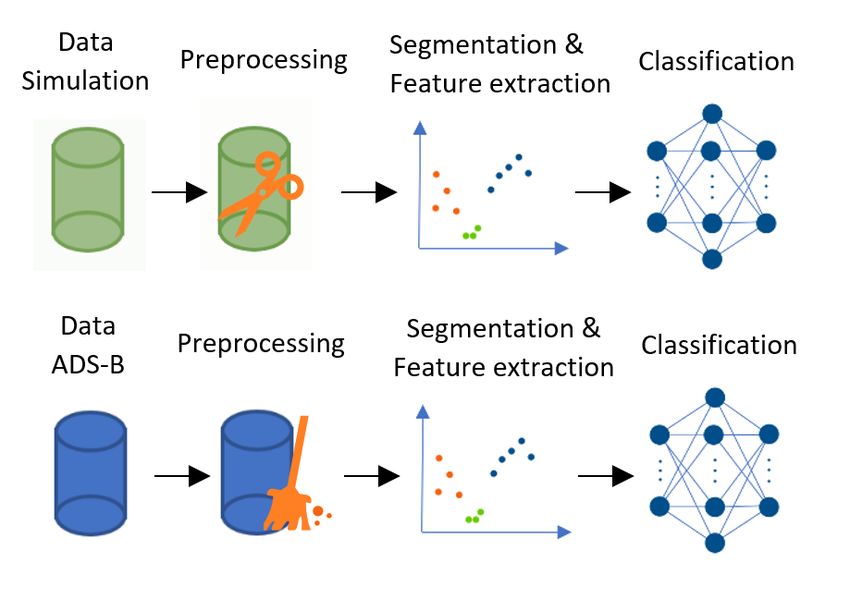
Abstract

Abstract
Flight phases are essential for many applications of aviation research. In this
project, a novel machine learning model for the identification of flight phases is
presented. The identification is performed on aircraft trajectory data, which in
contrast to other flight data, is a publicly available resource obtained through the
Automatic Dependent Surveillance Broadcast (ADS-B) concept. With the help
of supervised simulation data, a model that aims at improving state-of-the-art
flight phase identification on trajectory data is developed. The model combines K-
means clustering, allowing the segmentation to capture transitions between phases
more closely, with a Long Short-Term Memory (LSTM) network, able to learn the
dynamics of a flight. The improvement of this work, compared with the state-of-
the-art model by Sun et al. [41] based on fuzzy logic, comprises: increasing the
accuracy by more than 2%, adhering to the International Civil Aviation Organ-
isation (ICAO) standard, and increasing the number of flight phases to include
take-off, landing, and others. The latter shows potential, considering the perfor-
mance on simulation data, however, requires more realistic training data to achieve
similar performance on actual flights.

                                        IV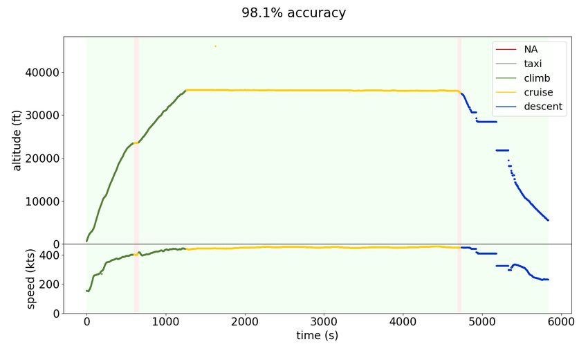
Contents

   Abstract                                                                                                          IV

   List of Figures                                                                                                   VII

   List of Tables                                                                                                    IX

1 Introduction                                                                                                         1
  1.1 Aviation . . . . . . . . . . . . . . . . . . .         .   .   .   .   .   .   .   .   .   .   .   .   .   .     2
       1.1.1 Flight Phases . . . . . . . . . . . .           .   .   .   .   .   .   .   .   .   .   .   .   .   .     2
       1.1.2 Flight Trajectory Data . . . . . . .            .   .   .   .   .   .   .   .   .   .   .   .   .   .     3
  1.2 Machine Learning . . . . . . . . . . . . . .           .   .   .   .   .   .   .   .   .   .   .   .   .   .     4
       1.2.1 Clustering . . . . . . . . . . . . . .          .   .   .   .   .   .   .   .   .   .   .   .   .   .     4
       1.2.2 Density-based Clustering . . . . . .            .   .   .   .   .   .   .   .   .   .   .   .   .   .     6
       1.2.3 Long Short-Term Memory (LSTM)                   .   .   .   .   .   .   .   .   .   .   .   .   .   .     6

2 Related Work                                                                                                         9
  2.1 Flight phase estimation with fuzzy logic . . . . . . . . . . . . . . .                                          11
  2.2 Other machine learning models . . . . . . . . . . . . . . . . . . . .                                           13

3 Methods                                                                                                             15
  3.1 Data . . . . . . . . . . . . . . . . . .   .   .   .   .   .   .   .   .   .   .   .   .   .   .   .   .   .    16
      3.1.1 Broadcasted Trajectory Data          .   .   .   .   .   .   .   .   .   .   .   .   .   .   .   .   .    16
      3.1.2 Simulation Data . . . . . . . .      .   .   .   .   .   .   .   .   .   .   .   .   .   .   .   .   .    19
  3.2 The classifier . . . . . . . . . . . . .   .   .   .   .   .   .   .   .   .   .   .   .   .   .   .   .   .    23
      3.2.1 Segmentation . . . . . . . . .       .   .   .   .   .   .   .   .   .   .   .   .   .   .   .   .   .    23
      3.2.2 Features . . . . . . . . . . . .     .   .   .   .   .   .   .   .   .   .   .   .   .   .   .   .   .    25
      3.2.3 Classification . . . . . . . . .     .   .   .   .   .   .   .   .   .   .   .   .   .   .   .   .   .    26

4 Results                                                                                                             29
  4.1 Simulation Data . . . . . . . . . . .   . . . .        .   .   .   .   .   .   .   .   .   .   .   .   .   .    30
      4.1.1 Different data cuts . . . . .     . . . .        .   .   .   .   .   .   .   .   .   .   .   .   .   .    30
      4.1.2 Different penalty influence .     . . . .        .   .   .   .   .   .   .   .   .   .   .   .   .   .    32
      4.1.3 Segmentation . . . . . . . .      . . . .        .   .   .   .   .   .   .   .   .   .   .   .   .   .    33
  4.2 Broadcasted Trajectory Data . . .       . . . .        .   .   .   .   .   .   .   .   .   .   .   .   .   .    35
      4.2.1 Comparison with fuzzy logic       model          .   .   .   .   .   .   .   .   .   .   .   .   .   .    39

                                        V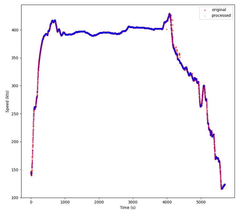
Contents

5 Conclusion                                                                                                    43
  5.1 Benefits of the model . . . . . . . . . . .   .   .   .   .   .   .   .   .   .   .   .   .   .   .   .   43
  5.2 Limitations of the model . . . . . . . . .    .   .   .   .   .   .   .   .   .   .   .   .   .   .   .   44
  5.3 Future Work . . . . . . . . . . . . . . . .   .   .   .   .   .   .   .   .   .   .   .   .   .   .   .   46
      5.3.1 Supplementary Real Flight Data          .   .   .   .   .   .   .   .   .   .   .   .   .   .   .   46
      5.3.2 Feature Improvement . . . . . . .       .   .   .   .   .   .   .   .   .   .   .   .   .   .   .   46
  5.4 Applications in Other Fields of Research      .   .   .   .   .   .   .   .   .   .   .   .   .   .   .   47

Acronyms                                                                                                        49

Bibliography                                                                                                    53

                                      VI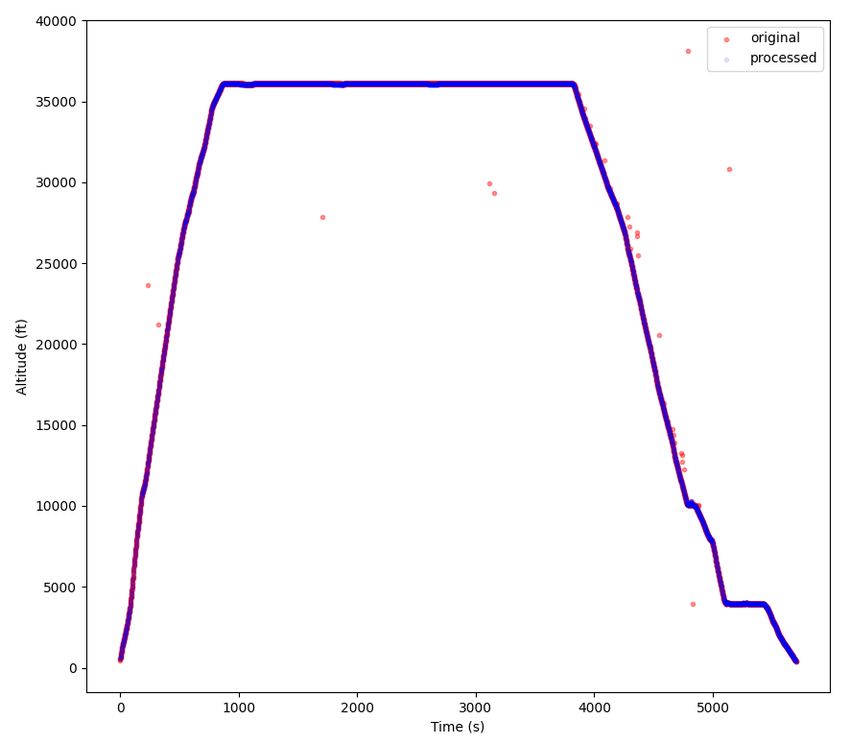
List of Figures
1.1 Flight phase progression over time relative to altitude. . . . . . . . 2
1.2 The structure of NN, RNN hidden nodes, and LSTM hidden nodes. 6
2.1 Membership functions used for flight phase estimation by Sun et al.
[41]. . . . . . . . . . . . . . . . . . . . . . . . . . . . . . . . . . . . 11
2.2 Valid transitions between flight phases according to Sun et al. [41]. . 11
2.3 Flight phases estimated as by Sun et al. [41] on sample data provided. 12
3.1 Structure of the model with different data sources. . . . . . . . . . . 15
3.2 Comparison between original noisy data and preprocessed data. . . 17
3.3 Classification error introduced through segmentation for different
number of clusters. . . . . . . . . . . . . . . . . . . . . . . . . . . . 24
4.1 Validation accuracies, loss, and loss penalty influence during train-
ing of 3500 epochs with penalty (α = 4) and without. . . . . . . . . 33
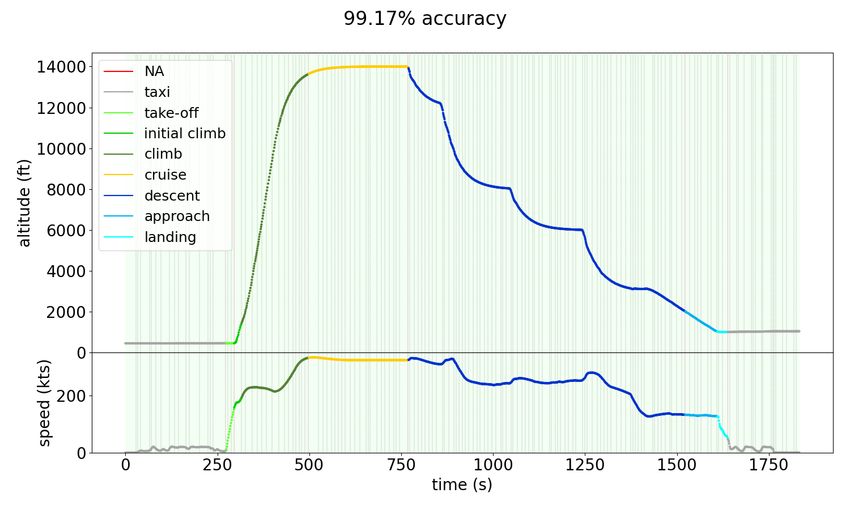
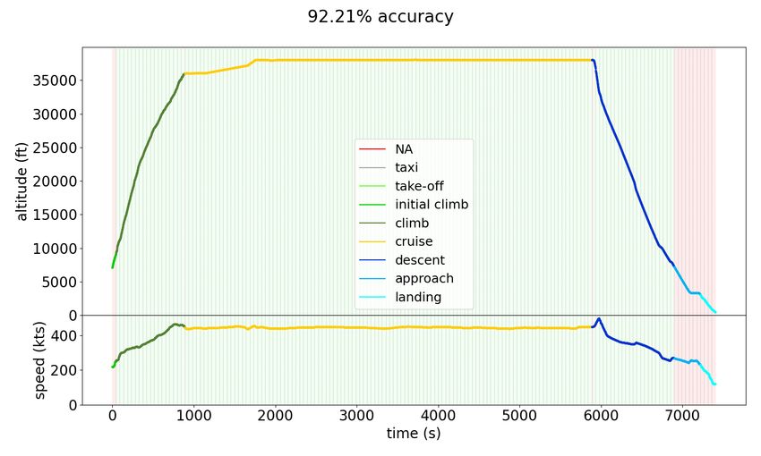
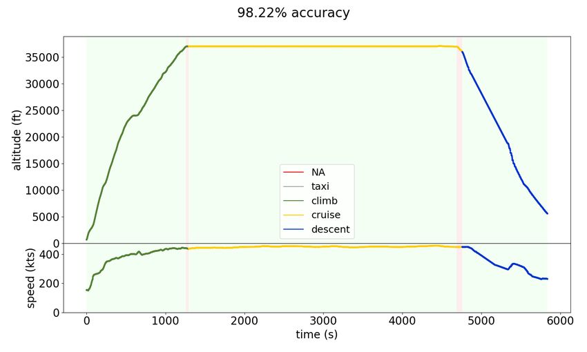
4.2 Results of the model with K-means segmentation and loss penalty. . 37
4.3 Classification performance on a noisy flight: comparison between
fuzzy logic [41] and this work. . . . . . . . . . . . . . . . . . . . . . 41
5.1 Comparison between computed rate of climb and original rate of
climb variable. . . . . . . . . . . . . . . . . . . . . . . . . . . . . . . 47
VII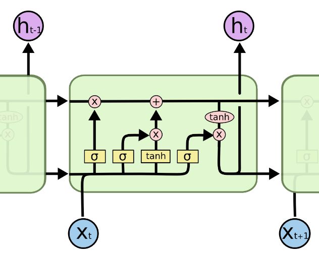
List of Figures

                  VIII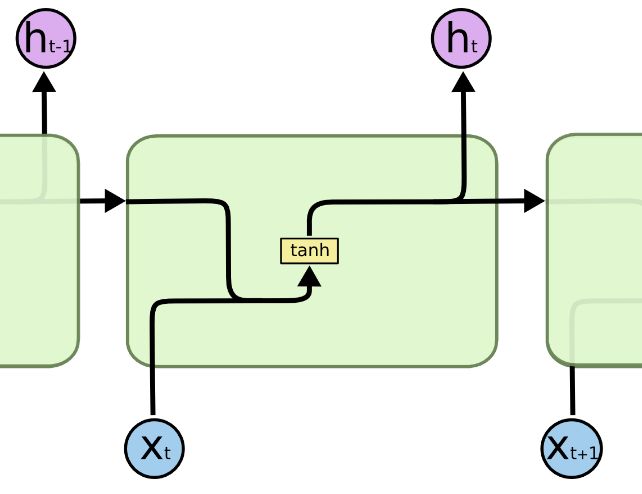
List of Tables

 2.1   Comparison of variables used and phases identified by related work
       and this work. . . . . . . . . . . . . . . . . . . . . . . . . . . . . . .     10

 3.1   Quality Statement of ADS-B flights. . . . . . . . . . . . . . . . . .          18
 3.2   Flight phases used in this work combined as compared to ICAO
       ADREP. . . . . . . . . . . . . . . . . . . . . . . . . . . . . . . . . .       20
 3.4   The rules applied for the rule based flight phase identification from
       aircraft variables. . . . . . . . . . . . . . . . . . . . . . . . . . . . .    22
 3.3   Aircraft state variables used in this work to label the data. . . . . .        22
 3.5   The average time, number of segments and time per segment of a
       flight phase in a full-length flight (flown in simulator). . . . . . . . .     24

 4.1   Influence of different data clippings on validation accuracy and test
       accuracy. . . . . . . . . . . . . . . . . . . . . . . . . . . . . . . . . .    31
 4.2   Influence of penalty on loss on identification performance. . . . . . .        32
 4.3   K-means segmentation compared to uniform segmentation on the
       simulation test data. . . . . . . . . . . . . . . . . . . . . . . . . . .      35
 4.4   The average time of a flight phase over different data clippings. . . .        36
 4.5   The models’ performance on ADS-B test data. . . . . . . . . . . . .            38
 4.6   Comparison of model in this work to the fuzzy logic approach by
       Sun et al. [41]. . . . . . . . . . . . . . . . . . . . . . . . . . . . . . .   40

                                         IX
List of Tables
XChapter 1
Introduction
Flight phases are part of the aircrafts state and essential for many applications of
aviation. Air traffic management uses flight phases in trajectory prediction [23],
which is essential for traffic flow prediction at airports and accident avoidance [39].
In aviation research, flight phases are, among other purposes, used to analyse and
reduce environmental impact [4, 10, 3]. The flight phase variable is either part of,
or computed on the aircrafts internal data which is very sensitive and has scarce
availability to the public. This is not the case for aircraft trajectory data. Sun et al.
[41] present a model for the identification of flight phases on large scale with only
trajectory data. This work uses internal aircraft data to label trajectory data and
develop a model that identifies flight phases with supervised learning, to answer
the following research question:
How much can the identification of flight phases using machine learning on
aircraft trajectory data be improved by supervised learning?
The identification consists of the following steps:
1. Data preprocessing
2. Data segmentation (K-means [28])
3. Segment feature extraction
4. Flight phase identification on segments (Long Short-Term Memory (LSTM)
[17])
5. Transfer flight phases from segments to original preprocessed data.
In this chapter, a brief description of flight phases is given together with an
introduction to using Automatic Dependent Surveillance Broadcast (ADS-B) tra-
jectory data and why it is important for the identification of these, after which
a background on the machine learning methods used in this work is provided. In
chapter 2 state-of-the-art flight phase identification from ADS-B trajectory data
based on fuzzy logic by Sun et al. [41] and other related work is presented. After-
wards, chapter 3 presents the details of this work’s model and chapter 4 discusses
1Chapter 1. Introduction
Figure 1.1: Flight phase progression over time relative to altitude.
the obtained results. Finally, the contributions of the model to aviation and ma-
chine learning research are evaluated and the possibilities of potential future work
are discussed.
1.1 Aviation
Each aircraft produces a lot of data during a flight, the majority of this data stays
within the aircraft during the flight and is later collected for post analysis by the
airline and the manufacturer of the aircraft. In this work, this data is referred
to as aircraft internal data and contains information regarding the flight phases.
However, in order to manage air traffic most aircrafts transmit information regard-
ing their trajectory, this data is received by other aircrafts but also by receivers
on ground making this data public. The internal aircraft data on the other hand
contains very sensitive information1 and is thus maintained private. This is why
research is aiming at enriching trajectory data [40] to allow for more data intensive
processing in the field of aviation, flight phases are at the basis of this as many
applications rely on them [43, 34, 49].
1.1.1 Flight Phases
Flight phases (also referred to as Phase of Flight or PoF) identify the operational
stages during an aircraft’s flight and are defined on board the aircraft and included
in the aircraft’s internal data. While there are multiple definitions and acronyms
for flight phases, the most commonly used are given by International Civil Aviation
Organisation (ICAO)’s Accident Data Reporting (ADREP) and International Air
Transport Association (IATA)2 [46] rather similar to each other, except for the
1
https://www.easa.europa.eu/domains/safety-management/safety-promotion/europe
an-operators-flight-data-monitoring-eofdm-forum accessed on: 15/03/2021
2
https://www.skybrary.aero/index.php/Flight Phase Taxonomy accessed on:
15/03/2021
21.1. Aviation
standing phase, which is not of interest to this work. This work focuses on the
definitions of the ICAO standard that provide a set of constraints on aircraft
parameters for each primary-phase and their sub-phases, the specifics of these
constraints and parameters, however, depend on the individual aircraft. By using
the ICAO standard, it will be possible to align this work with maintenance issues
and accident databases in future applications. As flight phases are used in post-
analysis, different models have been developed to estimate the flight phases based
on aircraft data or create simulations that include flight phases. These models often
generalise or group flight phases [41, 37, 44, 19, 23], as is done as well in this work.
Figure 1.1 shows a schematic overview of the progression of the flight phases used
in this work over time and relative to the aircrafts. A more technical definition of
the flight phases used in this work and their exact relation to the ICAO standard
will be given in chapter 3.
Applications of flight phases can be grouped in two main approaches: applica-
tions that focus on specific segments of the flight that correspond to one or more
flight phases and the analysis of the change to a parameter or behaviour during the
flight, comparing the different phases. The analysis of the environmental impact
of air traffic uses such segmentation and analyses mainly two sources: sound emis-
sion and fuel emission. Sound emission analysis requires a focus on the initial and
final phases as they are the ones closest to the earth [50]. Fuel emission analysis,
on the other hand, excludes these [15]. Flight segmentation is also necessary for
air traffic management purposes: aircraft initial mass estimation models either use
the climb phase [2] or the take-off phase [42], a more recent approach [43] instead
combines estimations on the different phases. As flight phases are characterised
by different events or parameter values, the comparison of the aircraft’s behaviour
during different phases is not only done for mass estimation but also for the anal-
ysis of the behaviour of pilots and crew during the flight or for accident analysis
and avoidance [1].
1.1.2 Flight Trajectory Data
The vast majority of aircrafts broadcast information about their trajectories, which
contain information to determine their current position and path. This information
is transmitted by means of ADS-B technology and received by ADS-B receivers
around the world. Currently in Europe over 82% of the aircrafts are equipped
with these transmitters and this number is expected to rise above 95% by 20253 .
The OpenSky Network [38] is one of the platforms using the ADS-B technology
to openly provide air traffic data for research purposes. This makes this data very
accessible and widely used. With ADS-B data the aircraft’s trajectory informa-
tion (position, altitude, velocity, and rate of climb), obtained from the different
systems inside the aircraft, is transmitted mostly every second together with the
information needed to identify the aircraft and the transmission.
OpenSky collects data from various receivers worldwide and groups them into
3
https://ads-b-europe.eu/ accessed on: 15/03/2021
3Chapter 1. Introduction
flights, as the signals acquired by the ADS-B receivers are obtained by multiple air-
crafts broadcasting their information, there can be interference between aircrafts.
This, combined with the internal errors and different sampling rates of the sensors
causes gaps in the data and noisy values (see figure 3.2). The quality of the data
thus varies from one flight to another, therefor, in this work, a quality statement
will be made regarding each analysed flight. Initial data preprocessing is thus nec-
essary to ensure that the quality of the input data is as high as possible. More
details on the processing of the data are provided in chapter 3.
1.2 Machine Learning
Machine learning algorithms are algorithms that learn from experience [29]. In
this study, two of the main categories of machine learning are used: supervised
learning algorithms and unsupervised learning algorithms. Supervised learning is
the machine learning task of learning by example: finding a mapping between input
and output by training on supervised data. In this work the input is the flight data
and the output is the flight phase. Supervised data consists of two components for
each element of the dataset: the input (xi ) and the corresponding labels (yi ), where
a label identifies the desired output that the model should produce from the input.
Different tasks can be performed with supervised learning. In this work, the focus
is on a classification task, as such the labels of the inputs consist of the class this
input belongs to (the flight phase). Once the supervised model is trained, it is able
to produce the correct output for new unlabeled inputs. A generalised supervised
learning algorithm can be seen as a black box that approximates a function:
G:X→Y
where X and Y are the input and output space respectively. The function is ap-
proximated by learning on a training set:
T = {(x0 , y0 ), ..., (xn , yn )}
The training set used for flight phase identification model consists of 256 flights
each divided into 160 segments where each segment is represented by 9 features
and is given a label corresponding to one of the 8 flight phases considered in this
work. As such X is a 256 × 160 × 9 matrix and Y a 256 × 160 matrix. The LSTM is
a supervised learning algorithm that will be described in more detail later in this
chapter. For unsupervised learning, the data is not enriched with a correct label.
As such unsupervised learning algorithms are used to find patterns or structures in
the data [5]. One of the main tasks suitable for unsupervised learning is clustering,
which is used in this work and described as follows.
1.2.1 Clustering
Clustering is the concept of putting together data points that are similar and sepa-
rating data points that are dissimilar. The similarity measure between data points
41.2. Machine Learning
and the representation of a cluster are the key differences between the various
clustering algorithms. In this work, two different clustering algorithms are used:
K-means [28] and Density-based Spatial Clustering of Applications with Noise
(DBSCAN) [14]. K-means is used to group together flight data points that are
similar into one segment, as similar data points belong to the same flight phase.
DBSCAN, on the other hand, is used in the last step of outlier removal, by group-
ing the data points belonging to the flight together and removing those that do
not (the outliers).
K-means
K-means [28] is a centroid-based clustering algorithm, meaning that a cluster is
represented by the centroid of the data points belonging to it. A centroid is identi-
fied with a distance similarity measure, in the majority of cases squared Euclidean
distance.
The standard K-means algorithm starts by randomly assigning each data point
to one of the K clusters, where K is a predetermined number. It then proceeds by
alternating the following two steps until convergence:
• Assigning each data point (x) to the cluster (C) with the nearest mean (µ).
∀i ∈ {1, ..., k}. Ci = {∀x ∈ data : ||x−µi ||2 ≤ ||x−µj ||2 ∀j ∈ {1, ..., k}∧j =
6 i}
(1.1)
• Update the clusters’ means (µ) based on the newly assigned data points
that compose them.
1 X
∀i ∈ {1, ..., k}. µi = xj (1.2)
|Ci | x ∈C
j i
The algorithm converges when no points are assigned to different clusters, in com-
parison to the previous iteration or until the predetermined maximum number of
iterations is reached.
In this work K-means is used for dividing a signal into K segments of variable
length, where K = 160. The data corresponds to a full flight and each data point
represents the speed and altitude of one second during the flight. Compared to the
standard K-means algorithm, the following differences are introduced:
• The clusters are initialised with uniform segmentation, dividing the signal
into K equally long segments.
• Only the edge points of each cluster are able to change their currently as-
signed cluster based on the nearest mean.
More details about the algorithm used are provided in chapter 3.
5Chapter 1. Introduction
1.2.2 Density-based Clustering
DBSCAN [14] is one of the most known algorithms for density-based clustering,
which relies on the idea that clusters consist of data space regions of high point
density. Clusters are defined with the concept of core points and reachability:
• Core points are data points that have at least the minimum amount of
points to constitute a cluster within the reach of the maximum distance,
where the minimum amount of points and the maximum distance are prede-
termined.
• A point is reachable from a core point if it is within the maximum distance
of it.
A cluster is composed by all core points reachable from one another and non-core
points reachable from these core points. In this work DBSCAN is used to cluster
together all the data points belonging to the flight as these will have other flight
data points in their vicinity since abrupt changes within one second are physically
impossible.
1.2.3 Long Short-Term Memory (LSTM)
The main component of the model presented in this work, the classifier, is given by
a Long Short-Term Memory (LSTM), a type of Artificial Neural Network (NN).
An Artificial Neural Network is a computational architecture that consists of layers
of nodes interconnected to each other by weighted edges, inspired by the neurons
and synapses of the biological brain [16].
(a) NN structure (b) RNN cell (c) LSTM cell
Figure 1.2: source for b and c: https://colah.github.io/ accessed on:
15/03/2021
Structure of Artificial Neural Network (NN), Recurrent Neural Network (RNN)
hidden nodes, and Long Short-Term Memory (LSTM) hidden nodes.
61.2. Machine Learning
Three types of layers compose an Artificial Neural Network as can be seen in
figure 1.2a:
• The input layer represents the input for which a result is to be computed.
The dimensionality of the input defines how many nodes are present in this
layer. Many applications require feature extraction and data scaling before
the raw data can be processed by the network, in this case each feature will
have its own node in the input layer which receives values between 0 and 1.
In this work, the features are the first and last values of a segment for each
trajectory component that has been scaled to fit the interval between 0 and
1, as will be further explained in chapter 3.
• The output layer contains the result of the computation, depending on the
task at hand the number of nodes and the meaning of their values vary. The
task addressed in this thesis is a classification task, meaning that the output
layer contains a node for each class, more specifically each possible flight
phase, that represents the likelihood of the input belonging to that class.
• Hidden layers are the layers between the input and output layer. The num-
ber of hidden layers together with the number of nodes in each layer define
the computational capacity of the NN. A simple task can be solved with a sin-
gle hidden layer, however, complex tasks require multiple of them, networks
with many hidden layers are called Deep Neural Networks.
For supervised learning tasks, a NN is trained by receiving feedback on the
output it produces through its computation and adjusting the weights between
the nodes accordingly. The difference between the produced output and the desired
output is computed with a loss function and is called the loss. The influence of
the loss of a single data entry on the adjustment of the weights is regulated by
the learning rate. This is generally done with backpropagation, where the loss is
computed on the output layer and from that the error of each node in the network
is traced back by using the current weights, these same weights are then adjusted
to minimize the node error.
There are many types of NNs, the one used in the model presented in this
thesis is a LSTM, a type of Recurrent Neural Network (RNN) [36]. RNNs have
the peculiarity of having a memory of the past inputs allowing them to handle
sequential data. When feeding a sequence of data to a RNN, the output of each
element of the sequence is computed not only on the current element but also
through the memory of the previous elements of the sequence. As each node passes
its computed value of the element (t − 1) in the sequence to the computation of
that same node on the next element (t) in the sequence, this value is stored in the
cell state, see figure 1.2b. A known problem of RNNs is their vanishing gradient,
this occurs as the network only receives feedback on the produced outputs once the
whole sequence has been processed. Once the feedback reaches the early elements
of the sequence, the influence is too small compared to the later elements as the
backpropagation has to unravel for each element in the sequence, making it hard
to learn long-term dependencies.
7Chapter 1. Introduction
The LSTM tackles this problem by introducing a long-term memory, the mem-
ory of an LSTM cell remains unchanged if not by changes applied through the
forget gate activation vector and the output gate activation vector, the two left-
most vertical lines in the LSTM cell (figure 1.2c). The result of each cell at each
element of the sequence is a weighted computation between the memory and the
direct input. In this work, the network receives a sequence of flight segments that
compose a full flight, which allows the network to learn dependencies over the full
flight, and returns the flight phases for each segment of the flight after having seen
a full flight.
8Chapter 2
Related Work
Flight phases are essential for many applications of aircraft research and air traffic
management. At the same time, they are defined on board the aircraft by the
pilot or by internal system parameters [9], which are mostly unavailable on a large
scale because of their confidentiality. This has called for the need to identify them
externally either online or offline. Recent research shows that machine learning
approaches outperform previous statistical modelling approaches [23]. However, the
number of phases identified is often reduced compared to the number of existing
phases, especially neglecting the takeoff, initial climb, approach and landing phases
where most accidents occur [1] and which are thus much needed for air traffic
management. The aim of this work is to increase the number of identified phases,
including takeoff and landing, while keeping a similar accuracy to state-of-the-
art flight phase identification from trajectory data. It is worth mentioning that
compared to other identifiers in this work, the climb and descent are not merely
given by a positive or negative rate of climb as is mostly done for simplification in
other models.
Tables 2.1a and 2.1b provide an overview of the different aircraft variables used
and the flight phases detected by the models referenced in this chapter and this
work. More information regarding the referenced models is provided as follows and
more details regarding the variables and phases used in this work are found in
chapter 3.
9Chapter 2. Related Work
(a) Trajectory variables used in related work
state variable Sun et al. [41] Liu et al. [26] Kovarik et al. [23] this work
Paglione et al. [32]
Altitude X X X X
Speed X X
Rate of Climb X X X*
XY coordinates X
Pitch, Roll and
True Heading angle X
Power Lever Angle X
Engine Fan Speed X
* Rate of Climb is computed from altitude
(b) Flight phases identified by related work
Kovarik et al. [23]
flight phase Sun et al. [41] Liu et al. [26] this work
Paglione et al. [32]
ground / taxi X X X X
take-off X
climb X X X X*
cruise X X** X** X
level X X** X** *
descent X X X X*
turn X***
landing X
* climb is further divided into initial climb and climb, descent is divided into descent and approach, level is
considered part of climb or descent
** cruise and level are considered the same phase
*** In a separate model than for the other phases
Table 2.1: Comparison of variables used and phases identified by related work
and this work. The Sun et al. [41] model is based on fuzzy logic. Liu et al. [26]
use a Gaussian Mixture Model. Kovarik et al. [23] compare 3 different models
using Support Vector Machine, Long Short-Term Memory, and Neural Ordinary
Differential Equations. Paglione et al. [32] use linear regression.
102.1. Flight phase estimation with fuzzy logic
2.1 Flight phase estimation with fuzzy logic
An approach to the identification of flight phases from ADS-B data has been pro-
vided by Sun et al.[41] based on Density-based Spatial Clustering of Applications
with Noise (DBSCAN) clustering[14] and fuzzy logic[48]. This model uses data
from a single ADS-B receiver, which means it has to process all raw broadcasted
messages and divide them into flight segments. This, together with denoising, is
done by standardization and clustering using DBSCAN. From these single flights,
it then estimates flight phases by applying fuzzy logic to flight segments of a fixed
number of seconds. Fuzzy logic introduces partial truth to Boolean logic: rather
than a statement being true or false, it can range anywhere in between these two
values. The truth value is called the degree of membership or membership value
of the input, which is calculated through the membership function. The trajec-
tory variables used by Sun et al. are: altitude (H), speed (V), and rate of climb
(RoC). Values of each of these variables are mapped to a membership value with
the membership functions in figure 2.1.
Figure 2.1: Membership functions used for Figure 2.2: Valid transitions be-
flight phase estimation by Sun et al. [41]. tween flight phases according to
The upper three graphs show the membership Sun et al. [41]: ground (GND),
functions for the region of values of each flight climb (CL), cruising (CR), de-
trajectory variable and the lower graph shows scending (DE), and levelling
the membership function for each phase given (LVL).
the logic statement that defines it.
11Chapter 2. Related Work
(a) Flight with valid phase transitions. (b) Flight with invalid phase transitions.
Figure 2.3: Flight phases estimated as by Sun et al. [41] on sample data provided.
Possible phases are ground (GND), climb (CL), cruising (CR), descending (DE),
levelling (LVL) or unknown (NA). The flight labeled with invalid transitions shows
a transition from climb to descent and from descent to cruise, both not valid.
The following logic is applied to define the flight phases are defined:
• Ground = Hgnd ∧ Vlo ∧ RoC0
• Climb = Hlo ∧ Vmid ∧ RoC+
• Cruise = Hhi ∧ Vhi ∧ RoC0
• Descent = Hlo ∧ Vmid ∧ RoC−
• Level f light = Hlo ∧ Vmid ∧ RoC0
To evaluate this model, Sun et al. count the number of invalid transitions, where
the valid transitions are the ones shown in figure 2.2. One could argue that the
image shows possible transitions from cruise to climb and from descent to climb,
which are not universally identified as possible transitions [9]. Of the 500 flights
used for validation, less than 5% had at least one invalid transition as defined
by the authors. The main disadvantage of this tool is that the number of flight
phases identified is rather small and with the available data, the takeoff and landing
phase could be identifiable using acceleration [41]. Figure 2.3 shows a positive and
negative example of the identification with the model obtained by execution of the
model and data given in their public repository1 .
1
https://github.com/junzis/flight-data-processor accessed on: 15/03/2021
122.2. Other machine learning models
2.2 Other machine learning models
A different model for flight phase estimation with machine learning has been pre-
sented by Liu et al., using a Gaussian Mixture Model (GMM) clustering [26]. This
unsupervised model offers nearly the same phases as the previously discussed model
by Sun et al. but rather than trajectory data, this model also uses aircraft internal
data such as: pitch angle, roll angle, true heading angle, power lever angle, and
engine fan speed.
There are also models that aim at predicting the phase of flight as part of
trajectory prediction. Kovarik et al. [23] compared 3 machine learning models for
this purpose to a simple regression model proposed by Paglione et al. [32]: Support
Vector Machine (SVM), Long Short-Term Memory (LSTM), and Neural Ordinary
Differential Equations (NODE). They found that the LSTM model performed best
among the 3 analysed. The LSTM model consists of two separate networks that
predict the next horizontal or vertical flight phase one step ahead. The horizontal
flight phases consist of straight and turn, however, the vertical flight phases consist
of ascending, descending, and level flights. These flight phases were predicted from
X and Y coordinates and altitude but do not specify the optimal window length
and or sequence length used by the LSTM.
The model in this work has combined the approach of clustering and LSTM.
Firstly, similar values are grouped together, as similar values often belong to the
same flight phase. In contrast to previous work, more clusters than the number of
flight phases are identified and kept continuous in time to give them to a LSTM
that learns the sequential dependencies of these clusters and identifies flight phases
with potentially multiple clusters. The details of this implementation are provided
in the next chapter.
13Chapter 2. Related Work
14Chapter 3
Methods
In this chapter the details of the implementation of the model and the data used
are described, a schematic overview can be seen in figure 3.1. First, the their
usage and labeling of the different sources of data are described. After which, the
various components of the model are described: segmentation, feature extraction,
and classification.
Figure 3.1: Structure of the model with different data sources, which require dif-
ferent preprocessing. ADS-B data contains noise originating from transmission
interference, different sampling rate of the sensors, and internal sensor errors. The
ADS-B data thus requires cleaning, which is done in the preprocessing. Simulation
data requires clipping in order to resemble the real data more closely, since the
data collected from flights is often incomplete.
15Chapter 3. Methods
3.1 Data
As internal aircraft data is scarce in availability, but required for the labeling of
the data, the model presented is trained on simulation data and evaluated both on
the simulation data itself and on the 7 real flights, of which both the broadcasted
trajectory data and the internal data, are available. These two sources differ in
their form of acquisition and thus require different preprocessing: the Automatic
Dependent Surveillance Broadcast (ADS-B) data mostly requires cleaning (see
subsection 3.1.1) and the simulation data clipping (see subsection 3.1.2) in order
to resemble the real data more closely.
3.1.1 Broadcasted Trajectory Data
ADS-B was developed as surveillance technology, able to provide easy access to
flight tracking and planning1 , at the same time . For this purpose aircrafts broad-
cast a message containing the message identification, flight identification (call sign),
GPS-derived latitude and longitude, barometric altitude, rate of climb, azimuth di-
rection and speed every one or two seconds. All flights considered in this work had
1 Hz transmissions, which is the most common transmission rate. The signals are
then acquired by the ADS-B receivers, which receive signals of multiple aircrafts
broadcasting their trajectory on the same channel. As such, there is some interfer-
ence between transmissions from different aircrafts [30]. This combined with the
internal errors from the sensors and sometimes different sampling rates is the cause
of gaps in the data and noise (see figure 3.2) [35].
Initial data preprocessing is thus necessary to ensure that the quality of the
input data is as high as possible. For this, outliers are removed, using filters and
density based clustering, after which the data is interpolated. The details of this
preprocessing are described in the following subsection. As the quality of the data
varies between flights, the data preprocessing also provides a quality statement for
each flight, airport and route. The quality statement can be used to find a relation
between the accuracy of the flight phase identification and the quality of the data.
Broadcast Data Preprocessing
As will be subsequently explained in this chapter, the ADS-B information of in-
terest to the model are the altitude and speed of the aircraft at each time point.
The following preprocessing steps are, hence, applied to these two variables.
At first, the invalid values in the data are removed. When a new value for a
variable is missing, the old one is repeated in the new transmission, these repeated
values are invalid data points. As such, the values that are identical to their pre-
decessors are removed. Since the values are given up to the 10th decimal in speed
and 2nd decimal for altitude, the event of two subsequent measurements produc-
ing the identical value is excluded. For the values that have valid predecessors,
outliers are removed based on a physically possible change within one second, the
1
https://ads-b-europe.eu/ accessed on: 15/03/2021
163.1. Data
transmission rate of the data of interest. For altitude this is 150 meters, while for
speed, 1.5 meters per second. This first step eliminates the majority of outliers
and is sufficient for the speed variable. However, the altitude variable is often more
noisy and in order to provide a more reliable interpolation, the second and third
steps further eliminate the remaining outliers.
The second step consists in applying the same thresholds as the first but this
time to the median of the 12 points before and after the point taken into con-
sideration. This allows to find outliers also where there are invalid points in the
vicinity of the outlier, or when there are multiple consecutive outliers. This method
is applied to the altitude variable since there are no valid sudden variations in it
which, instead, could occurs in the speed variable.
The third step consists in applying a density-based scanner (Density-based
Spatial Clustering of Applications with Noise (DBSCAN)) aimed at identifying
the main flight as a single cluster. This is done by providing relatively large hy-
perparameters. The minimum points to form a cluster is 75 and the maximum
distance between points is 300, based on Euclidean distance and calculated over
the 2 dimensions of time and altitude. At this point, less than 1% of flights have
visibly remaining outliers and the missing values are linearly interpolated between
two valid values.
Finally, the edges where either of the two variables presents missing data are
removed and the flights converted to a different metric system. For this application,
the Deutsches Zentrum für Luft- und Raumfahrt (DLR) prefers the use of feet (f t)
rather than meters (m) and knots (kts) rather than meters per second.(m/s).
(a) Altitude (b) Speed
Figure 3.2: Comparison between original noisy data in red and preprocessed in blue.
The original data has 30% missing values and 14% outliers, which are identified
and interpolated.
17Chapter 3. Methods
The preprocessing of steps for ADS-B data are defined as follows:
1. Removing values where difference within one second is larger than physically
possible.
(
N aN, if alt(t − 1) 6= N aN ∧ abs(alt(t) − alt(t − 1)) > 150 m
alt(t) =
alt(t), otherwise
(3.1)
(
N aN, if spd(t − 1) 6= N aN ∧ abs(spd(t) − spd(t − 1)) > 1.5 m/s
spd(t) =
spd(t), otherwise
(3.2)
2. Removing values where distance to the median over a window of empirically
found length is greater than the same threshold of the previous point.
NaN, if 12 ≤ t ≤ max(t) − 12 ∧
alt(t) = ∧abs(alt(t) − med(alt(t − 12, ..., t + 12))) > 150 m
alt(t), otherwise
(3.3)
3. Applying a density based clustering algorithm that identifies the main group
of data points and those outside it.
4. Linear interpolation for all points between two valid points.
5. Cutting off the edges where either of the used values presents invalid points.
This procedure was applied to 2088 flights, of which the summary of the quality
statement is reported in table 3.1. 7 of these flights had accompanying sensor data
that allows to label them.
The labeling is performed with the tool provided by the DLR described in sub-
section 3.1.2. This tool was developed for the real internal aircraft sensor data of
the DLR’s research aircraft and with some minor adjustments extended to pro-
vide the same labelling for the simulation data. Once the internal sensor data is
labeled, the two sources representing the same flight, the broadcasted trajectory
and the internal data, are aligned. At which point the labels are transferred from
the internal flight data to the ADS-B data.
Average Min Max
Percentage of missing values 33% 20% 77%
Percentage of outliers 13% 0% 22%
Table 3.1: Quality Statement of 2088 ADS-B flights analysed.
183.1. Data
3.1.2 Simulation Data
As the number of available ADS-B flights with sensor data is limited, the X-plane2
flight simulator is used to produce additional sensor data which will be labeled
with the flight phase tool. In the X-plane flight simulator, an aircraft model can
be chosen and flown, the creators of this simulator claim that with the advanced
computation of aircraft forces, their flight model is much more detailed than what is
used by most other flight simulators. In fact the X-plane simulator software can be
used to create Federal Aviation Administration of the United States Department
of Transportation (FAA) certified34 training devices, which require detailed and
close to reality simulations. FAA approved training devices can, for example, be
used for pilot training.
For the collection of simulation data in this work, a Boeing 737, one of the
most commonly used commercial aircrafts5 , was flown by the artificial intelligence
pilot made available by the simulator. These flights have no corresponding ADS-B
data, however, the simulator provides the same trajectory information as ADS-B
and will thus be used for training the model. Although the two sources provide the
same values, there are differences that cause a decrease in performance on the real
data compared to the simulation data. The main difference is that the simulation
provides much smoother and clean data than the transmitted ADS-B data. This
is mainly due to the noise of the transmission itself but also because the simulator
flies without air traffic which can effect the maneuvers of the aircraft. More details
regarding the differences in the sources of data will be discussed in the following
chapters.
A total of 421 simulation flights were recorded, of which 256 were used for
training, 65 for validation and 100 for testing. Each of these flights contains the
variables necessary to label the data and the trajectory information needed by the
model.
Simulation Data Preprocessing
The simulation data includes the values of the aircraft state variables that can be
seen in table 3.3. The majority of the variables are solely needed for labeling the
data. As there is no unified or universal definition to quantitatively specify flight
phases, many phases of flight are descriptively defined without quantitative con-
straints on the aircraft state variables [12]. In this research the International Civil
Aviation Organisation (ICAO) standard is used and the definitions are translated
into specific aircraft state variables rules. The relation between the complete set
of ICAO Accident Data Reporting (ADREP) primary phases and sub-phases and
the phases used in this work can be seen in table 3.2.
2
https://www.x-plane.com/
3
https://www.x-plane.com/pro/certified/ accessed on: 15/03/2021
4
https://www.faa.gov/regulations policies/advisory circulars/index.cfm/go/do
cument.information/documentID/1034348 accessed on: 15/03/2021
5
https://centreforaviation.com/analysis/reports/aircraft-fleets-western-v-eas
terncentral-europe-airbus-leads-orders-410122 accessed on: 15/03/2021
19Chapter 3. Methods
The Standing phase is excluded because there are no ADS-B transmissions in
this phase. The Maneuvring primary phase and Holding sub-phase are excluded
as they are phases that do not occur in commercial aircrafts. The taxi, cruise,
approach, and landing phases are a combination of their sub-phases for simplicity.
The Go Around and Rejected Takeoff are infrequent sub-phases, which is why they
are grouped together with their more frequent counterparts.
ICAO primary phases ICAO sub-phases Phase in this work
Standing (STD) - -
Taxi to Runway
Taxi (TXI) Taxi to Takeoff Position taxi (TXI)
Taxi from Runway
Takeoff
Takeoff (TOF) take-off (TOF)
Rejected Takeoff
Initial Climb (ICL) - initial climb (ICL)
Climb to Cruise climb (CLI)
Cruise
cruise (CRZ)
En Route (ENR) Change of Cruise Level
Descent descent (DST)
Holding -
Aerobatics
Maneuvering (MNV) -
Low Flying
Initial Approach (IFR)
Circuit Pattern - Downwind
Approach (APR) -
Circuit Pattern - Base approach (APR)
Visual Flight Rules (VFR)
Circuit Pattern - Final
Circuit Pattern - Crosswind
Go Around
Flare
Landing (LDG) landing (LDG)
Landing Roll
Table 3.2: Flight phases used in this work combined as compared to ICAO ADREP.
The standing and maneuvring phases, together with the holding sub-phase, are
excluded for being out of the scope of this work. The taxi, approach, and landing
are a combination of their sub-phases for simplicity, with the exception of the go
around sub-phase which together with the rejected takeoff sub-phase are included
in their primary phase because of their infrequency.
The data labeling consists of applying a rule-based approach for flight phase
identification based on the ICAO standard. For this purpose, a tool has been devel-
203.1. Data
oped by the DLR6 to augment aircraft internal sensor data with the corresponding
flight phase as closely to the ICAO definitions as possible. The relation between
the rules used in this work and the ICAO nomenclature can be found in table 3.2.
This tool has been developed for an Airbus A320 aircraft7 for which the DLR has
access to some internal flight data (the 7 real flights used in this work). This tool
has been adapted to the X-plane simulation data of the Boeing 7378 as the state
variables for the two sources of data slightly differ. Table 3.3 shows the adapta-
tion made on the simulation data to fit the real data state variables. The specific
rules for each phase in this work are described in table 3.4 with the use of the
abbreviations given in table 3.3. In these tables, the altitude indicates altitude
above runway, the functions max(param), min(param), abs(param) indicate the
maximum, minimum or absolute value of that parameter and ts(event) indicates
the time frame (in seconds) of a certain event.
Descriptively, the flight phases of tables 3.2 and 3.4 are defined as follows:
• taxi (TXI): The phase before take-off or after landing when the engine is on
and the aircraft is on ground.
• take-off (TOF): The engine is at at least 80% of its maximum achieved during
the flight and the aircraft is below 35 feet above the runway.
• initial climb (ICL): From the end of the take-off phase until the altitude
reaches 1000 feet above the runway.
• climb (CLI): From the end of the initial climb phase until the cruise phase.
• cruise (CRZ): The altitude rate is near to 0 and the aircraft’s altitude is above
1000 feet altitude and one of the following conditions is true: the aircraft is
flying at near to maximum altitude or the altitude rate is near to 0 for more
than 6 minutes.
• descent (DST): The aircraft’s rate of climb is negative for more than 2 min-
utes and the approach phase has not yet started.
• approach (APR): The aircraft’s rate of climb is negative and the altitude is
below 1000 feet from the runway.
• landing (LDG): 5 seconds before the aircraft reaches the ground and until it
leaves the runway (i.e., when it starts steering) or stops.
6
developed by Alexander Kamtsiuris (alexander.kamtsiuris@dlr.de) in the department of Pro-
cess Optimisation and Digitalisation, part of the Maintenance Repair and Overhaul institute.
7
https://www.airbus.com/aircraft/passenger-aircraft/a320-family.html accessed
on: 15/03/2021
8
https://www.boeing.com/history/products/737-classic.page accessed on: 15/03/2021
21Chapter 3. Methods
Flight Phase Rule
TXI gear compr ∧ tgt epr > 0 ∧ (ts < ts(T OF ) ∨ ts > ts(LDG))
TOF alt > 35 ∧ gear lvr down ∧ cmd epr · tgt epr > 0.8 · max(tgt epr)
ICL ts > ts(T OF ) ∧ 35 < alt < 1000
CLI ts > ts(ICL) ∧ ts < ts(CRZ)
CRZ −500 < roc < 500 ∧
∧ ((alt > max(alt) − 1000) ∨ (alt > 1000 ∧ (tsend − tsbegin ) > 360))
DST roc < −10 ∧ (tsbegin − tsend ) > 120 ∧ ts < ts(AP R)
APR roc < −10 ∧ alt < 1000
LDG ts > ts(T OF ) ∧ tsbegin − ts(gear compr) < 5 ∧
∧ (abs(steer ang) < 3 ∨ spd == 0)
Table 3.4: The rules applied for the rule based flight phase identification from
aircraft variables.
Measurement Labeling (L) /
State Variable Abbreviation Unit Conversion
Conversion (C)
Time ts seconds L -
Barometric altitude alt feet L -
Ground Speed spd knots L -
alt
Altitude Rate roc feet per minute L
ts
Target Take-off
tgt epr - L -
Engine Pressure Ratio
Throttle thro - C -
Commanded Take-off
cmd epr - L 1 + thro · (max(tgt epr) − 1)
Engine Pressure Ratio
Landing Gear Deployment gear lvr down boolean value L
Engine Normal Force norm pound C
(
T rue, if norm > 0
Force on Main Landing Gear gear compr boolean value L
F alse, if norm ≤ 0
(
steer ang, if gear comp
Nose Gear Steering Angle steer ang degrees L
0, if ¬gear comp
Table 3.3: Aircraft state variables used in this work to label the data: internal
aircraft values used for labeling (L) and the internal aircraft values used to convert
or compute (C) differing or missing values in the simulation data.
As ground data is not often available in ADS-B due to the complexity of trans-
mission such as obstacles, the flight data often does not include, or only partially
includes, phases that are close to the ground. These are the taxi, take-off, initial
climb, approach, and landing phases. For this purpose, the training and valida-
tion set of the simulation data has been replicated with different clippings in the
beginning and in the end to more closely resemble the ADS-B data.
223.2. The classifier
Each flight can thus appear in the following forms:
• Initial cut: an arbitrary point is chosen between the beginning of the take-off
phase and the end of the initial climb where the flight starts.
• Final cut: an arbitrary point is chosen between the beginning of the approach
phase and the end of the landing phase at which the flight ends.
• Dual cut: a flight has both an initial cut and a final cut.
• No cut: a flight is left intact.
In chapter 4 the effects of different combinations of cuts will be evaluated on the
validation set consisting of an equal distribution of these cuts and the real data.
3.2 The classifier
The model developed for the flight phase identification consists of two main steps:
the segmentation of the flight and the classification of the segments, after each
segment is translated into features. For the segmentation a variation of the K-
means clustering algorithm [28] is used, while for the classification a Long Short-
Term Memory (LSTM) [17] is used with a loss penalty function.
3.2.1 Segmentation
The first step of the model is the segmentation of the flight, which consists of
dividing it into a fixed number of segments. This is achieved by using a variation
of the K-means algorithm, further referred to as K-means segmentation.
K-means segmentation initializes segments by dividing the input into equal
parts after which it allows the edge points of segments to either belong to their
current segment or the neighboring one, based on their distance to the segment
means and if their current cluster has at least 4 points belonging to it. When two
neighboring edges both try to change their cluster of belonging, only the one that
has a bigger difference in distance between the two means is allowed to do so.
The hyperparameters of this algorithm are the number of clusters, the maxi-
mum number of iterations, and the weights used in the distance function:
• nclusters is found empirically with the right trade-off between size and the
minimum error introduced, it is set to 160. The mean error introduced by
the segmentation for the different values can be seen in figure 3.3
• The distance weights have been found with a parameter gridsearch. 10 weights
in the range (0,1] are considered for each of the trajectory variables. The op-
timal weights found for the minimum error introduced by segmentation were
0.1 altitude and 0.8 for speed.
• The maximum number of iterations is set by taking the 95th percentile of
iterations until convergence which corresponds to 100 iterations.
23Chapter 3. Methods
Flight phase time (s) segments segment time (s)
TXI 397 35.2 11.3
TOF 22 2.5 8.8
ICL 15 1.0 15
CLI 197 17.7 11.1
CRZ 174 13.0 13.4
DST 907 81.4 11.1
APR 70 5.8 12.1
LDG 30 3.4 8.8
Figure 3.3: Classification error in- Table 3.5: The average time, number of seg-
troduced through segmentation for ments and time per segment of a flight phase
different number of clusters, the in a full-length flight (flown in simulator).
number of segments used for the
model is marked in red.
The result is clusters that represent segments that are continuous in time, which
size varies with the amount of change over time. The pseudo code can be found in
algorithm 1 where:
1. x is the 2 dimensional input array of shape lengthf light × variablesf light , in
this case the number of variables is 2 (altitude and speed), each normalised
by variables subtracting that variable’s minimum of the flight and dividing
by the maximum of that variable in the flight.
2. c is the array of length lengthf light that indicates the cluster for each input
entry.
3. µ is the 2 dimensional array of shape numberclusters × variablesf light
4. div(x, y) is the integer division function.
5. mod(x, y) is the modulo operation.
6. get means(x, c) is the function that computes the means of each cluster.
7. dist(x, y) is the weighted Euclidean distance between two arrays of the same
shape.
The aim of this segmentation is to be able to reduce the error induced by phases
overlapping in a single segment. A change of flight phase most likely occurs at a
point where there is more change, i.e., where there is a bigger distance between
two consecutive data points.
243.2. The classifier
Algorithm 1 K-means segmentation
start ← 0
for i ← 1, ..., nclusters do
end ← start + div(lenx , nclusters )
if i ≤ mod(lenx , nclusters ) then
end ← end + 1
end if
c[start : end] ← i
start ← end
end for
µ ← get means(x, c)
c0 ← c
for iter ← 0, ..., niterations do
for i = 1, ..., f light len do
if counts(c0 , c[i]) > 4 then
if c[i] 6= c[i + 1] ∧ dist(x[i], µ[c[i + 1]]) < dist(x[i], µ[c[i]]) then
c0 [i] ← c[i + 1]
else if c[i] 6= c[i − 1] ∧ dist(x[i], µ[c[i − 1]]) < dist(x[i], µ[c[i]]) then
if c0 [i − 1] = c[i − 1] then
c0 [i] ← c[i − 1]
else if dist(x[i−1], µ[x[i−1]])−dist(x[i], µ[c[i−1]) < dist(x[i], µ[c[i]])−
dist(x[i], µ[c[i − 1]]) then
c0 [i] ← c[i − 1]
c0 [i − 1] ← c[i − 1]
end if
end if
end if
end for
c ← c0
µ ← get means(x, c)
end for
3.2.2 Features
After the flight has been divided into segments, these segments need to be given
to the classification network, this is achieved by extracting features from each
segment. As has been mentioned previously, the aircraft state variables given to the
model are altitude and speed, together with time. Other models [41, 23] also used
the rate of climb and XY coordinates. The latitude and longitude provided in ADS-
B data can be transformed into XY coordinates [13]. Since both XY coordinates
and latitude and longitude are referenced to the earth, for the network to be able to
generalize flights from different airports, the origin coordinates are required. ADS-
B flights, however, are often incomplete which means that the origin coordinates
are not always available. It would be possible to retrieve the coordinates from the
25Chapter 3. Methods
origin airport, but this is out of the scope of this work. To circumvent this issue,
the latitude and longitude could be used taking their difference over time, yet this
would correspond to using the speed, as such, these variables are excluded in this
work. The rate of climb, on the other hand, is fairly easy to compute through the
difference in altitude, as such, rather than using the aircraft variable, it is directly
computed from the altitude and introduced as a feature, as has been done for the
labelling provided by DLR.
The following features given to the network are computed for each segment
provided by K-means segmentation:
1. length of the segment (n)
2. initial altitude (alt0 )
3. final altitude (altn )
4. initial speed (spd0 )
5. final speed (spdn )
6. initial rate of climb (alt1 − alt0 )
7. final rate of climb (altn − altn−1 )
Each of these features is normalised: for the first 5 features (length, altitude,
and speed), this consists in dividing each of them by the maximum value of that
feature in each flight. For the rate of climb features, this consists in subtracting the
minimum value of that feature in the flight it belongs to and subsequently dividing
it by the maximum. The altitude and speed are always positive, and if a flight is
incomplete, the minimum altitude or speed might not correspond to the value of
these in a complete flight.
3.2.3 Classification
The features extracted from the segments, as explained previously, are used by
the classification network that labels each segment with a flight phase. For the
classification, a neural network is needed that is able to capture longer temporal
relations of a flight. For this purpose, an Long-Short Term Memory (LSTM) model
suits this task as it was designed for this purpose [17]. The LSTM receives features
of the segments, described previously, as inputs and learns to classify the clusters
according to the prevailing label of that cluster. The Artificial Neural Network
(NN) is implemented in Pytorch [33] and consists of an input layer, 2 layers of 16
LSTM cells, followed by an activation layer consisting of the logarithm of a softmax
function. The output is a value between 0 and 1 for each of the classes, where 1
indicates the segment belongs to that class and 0 indicates that it does not belong
to that class. For training, a batch size of 16 and a negative log likelihood loss
(NLLL) are used for stochastic gradient descent. The overview of the architecture
26You can also read