Dmitri Krioukov CAIDA/UCSD - Hyperbolic geometry of complex networks

Hyperbolic geometry of complex networks

           Dmitri Krioukov
            CAIDA/UCSD
              dima@caida.org
          F. Papadopoulos, M. Boguñá,
             A. Vahdat, and kc claffy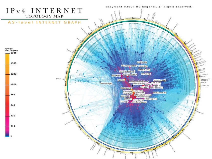

Complex networks
Technological             Can there be anything
„   Internet              common to all these
„   Transportation        networks???
„   Power grid
Social                    Naïve answer:
„   Collaboration         „   Sure, they must be complex
„   Trust                 „   And probably quite random
„   Friendship            „   But that’s it
Biological                Well, not exactly!
„   Gene regulation
„   Protein interaction
„   Metabolic
„   Brain

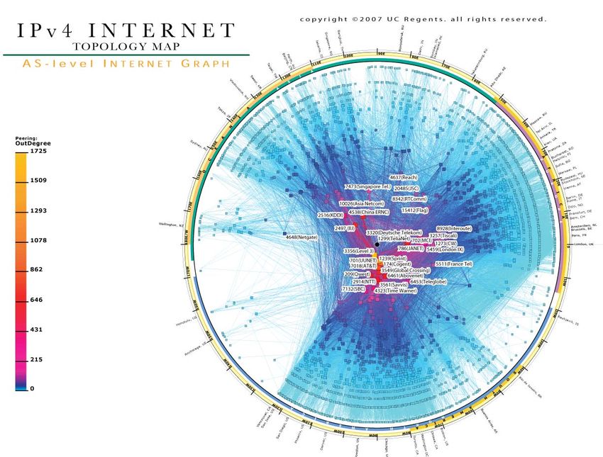
Internet
Heterogeneity:
distribution P(k)
of node degrees k:
 „   Real:   P(k) ~ k-g
 „   Random: P(k) ~ lke-l/k!
Clustering:
average probability that
node neighbors are connected:
 „   Real:   0.46
 „   Random: 6.8μ10-4

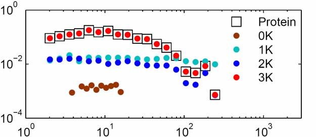
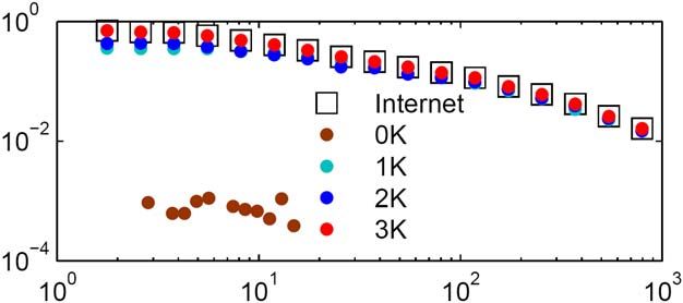
Internet vs. protein interaction

Strong heterogeneity and clustering as
common features of complex networks
 Network               Exponent of the     Average
                       degree distribution clustering
 Internet                     2.1             0.46

 Air transportation           2.0             0.62

 Actor collaboration          2.3             0.78

 Protein interaction          2.4             0.09

 Metabolic                    2.0             0.67

 Gene regulation              2.1             0.09

Any other common features?
Heterogeneity, clustering, some randomness, and
their consequences:
„   Small-world effect (prevalence of short paths)
„   High path diversity (abundance of different paths
    between the same pair of nodes)
„   Robustness to random breakdowns
„   Fragility to targeted attacks
„   Modular/hierarchical organization
pretty much exhaust all the commonalities—the
networks are quite different and unique in all other
respects
Can we explain these two fundamental common
features, heterogeneity and clustering?

Hidden metric space explanation
All nodes exist in a metric space
Distances in this space abstract node
similarities
„   More similar nodes are closer in the space
Network consists of links that exist with
probability that decreases with the hidden
distance
„   More similar/close nodes are more likely to be
    connected

Mathematical perspective:
Graphs embedded in manifolds

All nodes exist in “two places at once”:
„ graph
„ hidden metric space, e.g., a Riemannian manifold

There are two metric distances between each
pair of nodes: observable and hidden:
„ hop length of the shortest path in the graph
„ distance in the hidden space

Hidden space visualized

Hidden metric spaces explain the
complex network structure

Clustering is a consequence of the metric
property of hidden spaces
Heterogeneity is a consequence of their
negative curvature (hyperbolic geometry)

Hidden metric spaces explain the
complex network function

Transport or signaling to specific destinations is
a common function of many complex networks:
„   Transportation
„   Internet
„   Brain
„   Regulatory networks
But in many networks, nodes do not know the
topology of a network, its complex maze

Complex networks
as complex mazes
To find a path through a
maze is relatively easy if
you have its plan
Can you quickly find a
path if you are in the maze
and don’t have its plan?
Only if you have a
compass, which does not
lead you to dead ends
Hidden metric spaces are
such compasses

Milgram’s experiments
Settings: random people were asked to forward a
letter to a random individual by passing it to their
friends who they thought would maximize the
probability of letter moving “closer” to the
destination
Results: surprisingly many letters (30%) reached
the destination by making only ~6 hops on
average
Conclusion:
„   People do not know the global topology of the human
    acquaintance network
„   But they can still find (short) paths through it

Navigation by greedy routing
To reach a destination, each node forwards
information to the one of its neighbors that
is closest to the destination in the hidden
space

Hidden space visualized

Result #1:
Hidden metric spaces do exist

Their existence appears as the only
reasonable explanation of one peculiar
property of the topology of real complex
networks – self-similarity of clustering

                     Phys Rev Lett, v.100, 078701, 2008

Result #2:
Complex network topologies are navigable

Specific values of degree distribution and
clustering observed in real complex
networks correspond to the highest
efficiency of greedy routing
Which implicitly suggests that complex
networks do evolve to become navigable
Because if they did not, they would not be
able to function

                      Nature Physics, v.5, p.74-80, 2009

Real networks are navigable

Result #3:
Successful greedy paths are shortest

Regardless the structure of the hidden
space, complex network topologies are
such, that all successful greedy paths are
asymptotically shortest
But: how many greedy paths are successful
does depend on the hidden space geometry

                    Phys Rev Lett, v.102, 058701, 2009

Result #4:
In hyperbolic geometry, all paths are successful

Greedy routing in complex networks, including the
real AS Internet, embedded in hyperbolic spaces, is
always successful and always follows shortest paths
Even if some links are removed, emulating topology
dynamics, greedy routing finds remaining paths if
they exist, without recomputation of node coordinates
The reason is the exceptional congruency between
complex network topology and hyperbolic geometry

Result #5:
Emergence of topology from geometry

The two main properties of complex
network topology are direct consequences
of the two main properties of hyperbolic
geometry:
„ Scale-free degree distributions are a
  consequence of the exponential expansion of
  space in hyperbolic geometry
„ Strong clustering is a consequence of the fact
  that hyperbolic spaces are metric spaces

                        Phys Rev E, v.80, 035101(R), 2009

Motivation for hyperbolic spaces
under complex networks

Nodes in complex networks can often be
hierarchically classified
„   Community structure (social and biological networks)
„   Customer-provider hierarchies (Internet)
„   Hierarchies of overlapping balls/sets (all networks)
Hierarchies are (approximately) trees
Trees embed almost isometrically in hyperbolic
spaces

Mapping between balls B(x,r) in d
and points α = (x,r) in d+1

                      If |α-α'| § C, then
                      there exist k(C) s.t.
                      k-1 § r/r' § k and
                      |x-x'| § k r
                      If |x-x'| § k r and
                      k-1 § r/r' § k, then
                      there exist C(k) s.t.
                      |α-α'| § C

Metric structure of hyperbolic spaces
The volume of balls and surface of spheres grow
with their radius r as
                         eαr
where α = (–K)1/2(d–1), K is the curvature and d is
the dimension of the hyperbolic space
The numbers of nodes in a tree within or at r hops
from the root grow as
                         br
where b is the tree branching factor
The metric structures of hyperbolic spaces and
trees are essentially the same (α = ln b)

Hidden space in our model:
hyperbolic disc

Hyperbolic disc of radius R, where
N = c eR/2, N is the number of nodes in the
network and c controls its average degree
Curvature K = -1

Node distribution in the disc:
uniform

Uniform angular density
              rq(q) = 1/(2p)
Exponential radial density
    r(r) = sinh r / (cosh R – 1) ≈ er-R

Connection probability:
step function

Connected each pair nodes located at (r,q)
and (r',q'), if the hyperbolic distance x
between them is less than or equal to R,
where

 cosh x = cosh r cosh r' - sinh r sinh r' cos Dq

Average node degree at distance r
from the disc center

Average node degree at distance r
from the disc center
Terse but exact expression

Simple approximation:
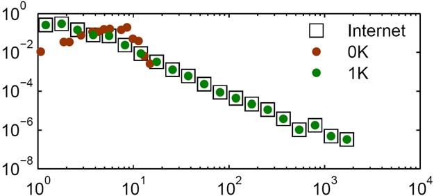
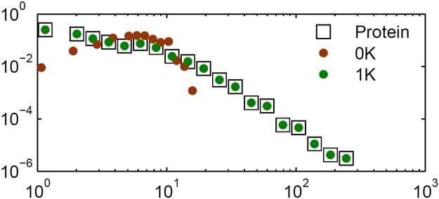
          k(r) ≈ (4c/p) e(R-r)/2

Degree distribution
Since r(r) ~ er and k(r) ~ e-r/2,
        P(k) = r[r(k)] |r'(k)| ~ k-3
Power-law degree distribution naturally
emerges as a simple consequence of the
exponential expansion of hyperbolic space

Generalizing the model
Curvature
                   K = - z2
and node density:
                r(r) ≈ a ea(r-R)
lead to the average degree at distance r
         k(r) ~ e-zr/2      if a/z ¥ 1/2; or
         k(r) ~ e- ar/2     otherwise

Generalized degree distribution
Degree distribution
                 P(k) ~ k-g
where
        g = 2 a/z + 1      if a/z ¥ 1/2
        g=2                otherwise
Uniform node density (a = z) yields g = 3 as
in the standard preferential attachment

Node degree distribution:
theory vs. simulations

The other way around
We have shown that scale-free topology
naturally emerges from underlying
hyperbolic geometry
Now we will show that hyperbolic
geometry naturally emerges from scale-free
topology

The 1 model
The hidden metric space is a circle of radius
                     N/(2p)
The node density is uniform (=1) on the circle
Nodes are assigned an additional hidden variable
k, the node expected degree, drawn from
                 rk(k) = (g-1)k-g
To guarantee that k(k) = k, the connection
probability must be an integrable function of
                  c ~ NDq /(kk')
where Dq is the angle between nodes, and k, k' are
their expected degrees

The 1-to-2 transformation
Formal change of variables
k = ez(R-r)/2            (cf. k(r) ~ e-zr/2 in 2)
where
z/2 = a/(g-1)            (cf. g = 2 a/z + 1 in 2)
yields density
r(r) = a ea(r-R)         (as in 2)
and the argument of the connection probability
                    c = ez(x-R)/2
where
              x = r + r' + (2/z) ln(Dq/2)
is approximately the hyperbolic distance between
nodes on the disc

Fermi connection probability
Connection probability can be any function of c
Selecting it to be 1 / (1 + c1/T), T ¥ 0, i.e.,
           p(x) = 1 / (1 + ez(x-R)/(2T))
allows to fully control clustering between its
maximum at T = 0 and zero at T = 1
At T = 0, p(x) = Q(R-x), i.e., the step function
At T = 1 the system undergoes a phase transition,
and clustering remains zero for all T ¥ 1
At T = ¶ the model produces classical random
graphs, as nodes are connected with the same
probability independent of hidden distances

Physical interpretation
Hyperbolic distances x are energies of
corresponding links-fermions
Hyperbolic disc radius R is the chemical
potential
Clustering parameter T is the system
temperature
Two times the inverse square root of
curvature 2/z is the Boltzmann constant

Hyperbolic embedding
of real complex networks

Measure the average degree, degree
distribution exponent, and clustering in a
real network
Map those to the three parameters in the
model (c, a/z, T)
Use maximum-likelihood techniques (e.g.,
the Metropolis-Hastings algorithm) to find
the hyperbolic node coordinates

Navigation in 1 and 2
The 1 and 2 models
are essentially                Embedded Synthetic
equivalent in terms of         Internet networks
produced network
topologies
But what distances, 1
                          1    76%      § 70%
or 2, should we use to
navigate the network?     2    95%      § 100%
Successful greedy paths
are asymptotically
shortest
But what about success
ratio?

Visualization of a modeled network

Successful greedy paths

Unsuccessful greedy paths

Robustness of greedy routing in 2
w.r.t. topology perturbations

As network topology changes, the greedy
routing efficiency deteriorates very slowly
For example, for synthetic networks with
g § 2.5, removal of up to 10% of the links
from the topology degrades the percentage
of successful path by less than 1%

Why navigation in 2
is better than in 1
Because nodes in the 1 model are not connected
with probability which depends solely on the 1
distances NDq
Those distances are rescaled by node degrees to
c ~ NDq /(kk'), and we have shown that these
rescaled distances are essentially hyperbolic if
node degrees are power-law distributed
Intuitively, navigation is better if it uses more
congruent distances, i.e., those with which the
network is built

2
             10

                  2

1

    20

2
             10

                  2

1

    20

Shortest paths in scale-free graphs
and hyperbolic spaces

In summary
Hidden hyperbolic metric spaces explain, simultaneously, the
two main topological characteristics of complex networks
„   scale-free degree distributions (by negative curvature)
„   strong clustering (by metric property)
Complex network topologies are congruent with hidden
hyperbolic geometries
„   Greedy paths follow shortest paths that approximately follow shortest
    hidden paths, i.e., geodesics in the hyperbolic space
     „   Both topology and geometry are tree-like
This congruency is robust w.r.t. topology dynamics
„   There are many link/node-disjoint shortest paths between the same source
    and destination that satisfy the above property
     „   Strong clustering (many by-passes) boosts up the path diversity
„   If some of shortest paths are damaged by link failures, many others
    remain available, and greedy routing still finds them

Conclusion
To efficiently route without topology
knowledge, the topology should be both
hierarchical (tree-like) and have high path
diversity (not like a tree)
Complex networks do borrow the best out of
these two seemingly mutually-exclusive worlds
Hidden hyperbolic geometry naturally explains
how this balance is achieved

Applications
Greedy routing mechanism in these settings may
offer virtually infinitely scalable information
dissemination (routing) strategies for future
communication networks
„   Zero communication costs (no routing updates!)
„   Constant routing table sizes (coordinates in the space)
„   No stretch (all paths are shortest, stretch=1)
Interdisciplinary applications
„   systems biology: brain and regulatory networks, cancer
    research, phylogenetic trees, protein folding, etc.
„   data mining and recommender systems
„   cognitive science