Drivers and projections of global surface temperature anomalies at the local scale - IOPscience
←
→
Page content transcription
If your browser does not render page correctly, please read the page content below
LETTER • OPEN ACCESS

Drivers and projections of global surface temperature anomalies at the
local scale
To cite this article: Susanne A Benz et al 2021 Environ. Res. Lett. 16 064093

View the article online for updates and enhancements.

                               This content was downloaded from IP address 46.4.80.155 on 15/08/2021 at 22:20
Environ. Res. Lett. 16 (2021) 064093 https://doi.org/10.1088/1748-9326/ac0661
LETTER
Drivers and projections of global surface temperature anomalies
OPEN ACCESS
at the local scale
RECEIVED
16 February 2021 Susanne A Benz1,∗, Steven J Davis2 and Jennifer A Burney1,∗
REVISED 1
25 May 2021 School of Global Policy and Strategy, University of California San Diego, La Jolla, CA, United States of America
2
Department of Earth System Science, University of California Irvine, Irvine, CA, United States of America
ACCEPTED FOR PUBLICATION ∗
27 May 2021
Authors to whom any correspondence should be addressed.
PUBLISHED
E-mail: sabenz@ucsd.edu and jburney@ucsd.edu
17 June 2021
Keywords: urban heat, surface energy balance, land surface temperatures, urbanization scenarios, heat mitigation
Original Content from Supplementary material for this article is available online
this work may be used
under the terms of the
Creative Commons
Attribution 4.0 licence. Abstract
Any further distribution More than half of the world’s population now lives in urban areas, and trends in rural-to-urban
of this work must
maintain attribution to migration are expected to continue through the end of the century. Although cities create
the author(s) and the title
of the work, journal efficiencies that drive innovation and economic growth, they also alter the local surface energy
citation and DOI. balance, resulting in urban temperatures that can differ dramatically from surrounding areas. Here
we introduce a global 1 km resolution data set of seasonal and diurnal anomalies in urban surface
temperatures relative to their rural surroundings. We then use satellite-observable parameters in a
simple model informed by the surface energy balance to understand the dominant drivers of
present urban heating, the heat-related impacts of projected future urbanization, and the potential
for policies to mitigate those damages. At present, urban populations live in areas with daytime
surface summer temperatures that are 3.21 ◦ C (−3.97, 9.24, 5th–95th percentiles) warmer than
surrounding rural areas. If the structure of cities remains largely unchanged, city growth is
projected to result in additional daytime summer surface temperature heat anomalies of 0.19 ◦ C
(−0.01, 0.47) in 2100—in addition to warming due to climate change. This is projected to raise the
urban population living under extreme surface temperatures by approximately 20% compared to
current distributions. However we also find a significant potential for mitigation: 82% of all urban
areas have below average vegetation and/or surface albedo. Optimizing these would reduce urban
daytime summer surface temperatures for the affected populations by an average of −0.81 ◦ C
(−2.55, −0.05).
1. Introduction potential consequences for city populations: atmo-
spheric UHIs increase vulnerability to heat-related
More humans now live in cities than in rural areas, morbidity and mortality (Patz et al 2005, Luber and
and urbanization is expected to intensify over the McGeehin 2008, Mora et al 2017) and affect the
next century (Grimm et al 2008). The concentra- energy demand and efficiency of the urban pop-
tion and density of humans in urban settlements has ulation through altered heating and cooling needs
driven innovation and economic growth by simul- (Santamouris 2014b).
taneously increasing the efficiency of human trans- Urban heat anomalies are usually quantified as
actions and interactions, and by providing returns UHI Intensities—the difference between the tem-
to scale on infrastructure investments (Hanson 2001, perature (atmospheric, surface, or groundwater) of
2005, Bettencourt et al 2007, Bettencourt 2013). a city as a whole and its surrounding rural back-
However, conversion of natural landscapes to urban ground (Howard 1818, Oke 1973, Kalnay and Cai
ones has also dramatically changed the urban energy 2003); recent studies have begun to assess the global
balance, resulting in different, often higher, local variability of surface UHI Intensities (Peng et al
temperatures experienced by inhabitants. This so- 2011, Chakraborty and Lee 2019) and the relation-
called urban heat island (UHI) effect has important ship of urban heat with factors like city size (Huang
© 2021 The Author(s). Published by IOP Publishing LtdEnviron. Res. Lett. 16 (2021) 064093 S A Benz et al
et al 2019, Manoli et al 2019) and climate (Scott et al Urban Center Database (Florczyk et al 2019). These
2018). However, this city-level metric is inadequate urban agglomerations, defined by UN’s Degree of
for characterizing the consequences of urban temper- Urbanization methodology, house a total of 2.288 bil-
ature anomalies at higher spatial resolution. Indeed, a lion people worldwide (hereafter, urban population).
number of localized studies have shown that within- Figure 1(B) shows LST anomalies at full resolution,
city variations in urban temperatures can be large along with several defined urban agglomerations; our
(Grimmond 2007), and larger-scale efforts have clas- ∆T algorithm is sensitive enough to detect smaller
sified UHIs of selected cities into local climate zones urban settlements outside of the major urban areas
to account for heterogeneity in the urban morpho- defined by the GHS Database.
logy and landscape characteristics (Stewart and Oke We find that 67% of all urban pixels (housing 75%
2012, Yang et al 2021). Yet to date, a comprehensive of the urban population) show daytime and night-
assessment of drivers and impacts of urban temper- time warming (upper right quadrants in figure 2(A)),
ature anomalies both within individual cities and at while 9% of urban pixels (5% of urban population)
global scale has been lacking. show warming only during daytime, and 19% (17%
Here we introduce a global assessment of of urban population) show warming only at night.
local (1 km) surface temperature anomalies (∆T). Globally, on average, each person living in an urban
We derive the average ∆T—total, seasonal, and area is exposed to annual mean surface temperature
diurnal—for the world over the past decade to anomalies of +2.11 ◦ C (−2.58, 7.10, 5th–95th per-
quantify the heat burden created by the current dis- centiles) during daytime (+3.21 ◦ C (−3.97, 9.24) in
tribution of human population and city structure. Summer and +0.94 ◦ C (−2.27, 5.24) in Winter) and
We then use a simple empirical model informed by +1.49 ◦ C (−0.20, 3.91) during nighttime (+1.70 ◦ C
the surface energy balance (Oke 1988) to test the (−0.18, 4.59) in Summer and +1.34 ◦ C (−0.75, 4.76)
physically-predicted relationships between local sur- in Winter). Presently, 55% of the urban population
face temperature anomalies and a set of observable lives in areas with average summer daytime surface
and scalable measures on a global scale. We combine temperatures greater than 35 ◦ C, compared to 33% of
these relationships with a set of potential urbaniz- people in rural areas. If cities did not create these sur-
ation futures to derive likely distributions of urban face temperature anomalies, only 23% of the urban
surface temperatures at the end of the century, and population would live under such extreme daytime
discuss their impact on the number of people living summer surface temperatures (figure 2(B)). Import-
under extreme temperatures. antly, this pixel-scale analysis reveals a much higher
population share in areas with extreme surface sum-
2. Global patterns of urban surface mer daytime temperatures: city-scale analysis under-
temperature anomalies estimates the population living in areas with summer
daytime temperatures above 35 ◦ C by 13% and for
We define ∆T for each 1 km pixel, i, as the difference areas above 38 ◦ C by 36% (figure 2(B)).
between local satellite-observed land surface temper- Worldwide urban daytime ∆T tends to be more
ature (LST) and the median LST of rural surrounding extreme than urban nighttime anomalies, with an
areas (Benz et al 2017): average of 1.46 ◦ C (−2.63, 5.83) compared to 1.00 ◦ C
(−0.48, 3.02). Similarly, urban summer ∆T is most
∆Ti = LSTi − median(LSTrural )i (1) extreme (daytime 2.14 ◦ C (−3.97, 8.05) and night-
time 1.21 ◦ C (−0.43, 4.03)). However, urban winter
LSTs are 10-year mean (2004–2014) seasonal daytime ∆T shows an increased range for nighttime (0.79 ◦ C
and nighttime surface temperatures from MODIS (Z (−1.00, 3.49)) and a decreased range for daytime
Wan 2015a, 2015b). (See supplement S1 (available (0.79 ◦ C (−2.07, 4.21)). For all seasons, the highest
online at stacks.iop.org/ERL/16/064093/mmedia) for urban daytime surface temperature anomalies are
more information on data used in this study. LST found in Japan, and Central and South America.
images have an error ⩽2 K—this error is not dis- Urban cooling is primarily observed in dry areas
played in our analysis). Rural background pixels for of central Asia, North Africa, and the Middle East
comparison are defined as those falling within a (figure 1(A)). Figures 1(B) and (S)3 show full resolu-
100 km distance of pixel i, with nighttime lights below tion images of several archetypal locations. Although
a defined threshold, and similar elevation and aspect substantially different in climate and absolute surface
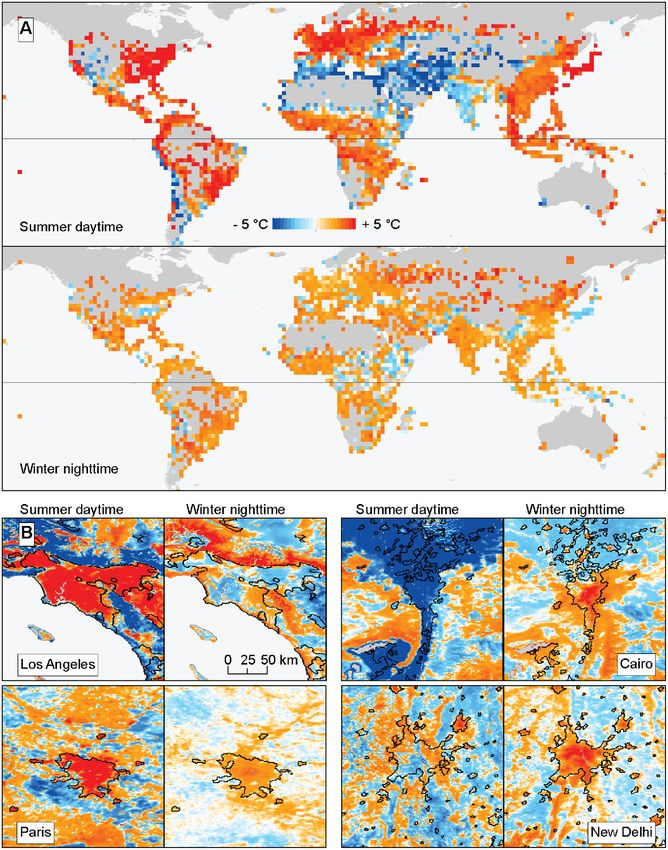
(see supplement 2.1). Figure 1(A) shows aggreg- temperatures, Parts of Los Angeles, California, US
ated global patterns of urban ∆T; our accompany- and Paris, France have summer daytime ∆T of more
ing app (https://sabenz.users.earthengine.app/view/ than 5 ◦ C, and reduced nighttime warming (with
surface-delta-t) shows full coverage and resolution. slight cooling in LA). Cairo, Egypt and New Delhi,
Although we calculate ∆T for all land areas, urban India are prime examples of urban cooling. Daytime
or rural, between −60◦ and 70◦ latitude, we high- summer LSTs in these cities are up to −5 ◦ C lower
light here a subset of 874 096 pixels (hereafter, urban than their background and ∆T becomes significant
pixels) defined by the Global Human Settlement only at night within the city centers.
2Environ. Res. Lett. 16 (2021) 064093 S A Benz et al
Figure 1. (A) Map of urban surface temperature anomalies (∆T). Shown is the average of all urban pixels in each grid cell
(aggregated to a 2◦ grid to show basic distribution). (Full 1 km resolution data are available at https://sabenz.users.
earthengine.app/view/surface-delta-t). Grid cells not included in a city defined by the Urban Center Database (Florczyk et al
2019) are left blank. (See figure S1 for all seasons and annual mean). (B) Summer daytime ∆T and winter nighttime ∆T for
selected locations. Shown are urban and non-urban ∆T, outlines of cities are shown in black.
Our data reveal large within-city variance in sur- 2.16), indicating the importance of analysis at local
face temperature anomalies. We calculate a global scales. We furthermore find qualitative evidence of
average standard deviation of ∆T within each city the differential impacts towards different communit-
to be 0.63 ◦ C (0.12, 1.62) for daytime and 0.34 ◦ C ies, with disadvantaged neighborhoods experiencing
(0.06, 0.85) for nighttime (figure 2(C)). Broken higher urban surface heat anomalies (figure S4) sup-
out by season, within-city daytime standard devi- porting claims by Chakraborty et al (2019) and
ation in ∆T increases in summer to 0.84 ◦ C (0.17, Benz and Burney (2021).
3Environ. Res. Lett. 16 (2021) 064093 S A Benz et al
Figure 2. (A) Heat map of daytime and nighttime urban surface temperature anomalies (∆T) averaged over the whole year, and
broken out by season (see figure S2 for spring and fall). Black markings indicate the mean point and 90% confidence ellipse. The
total area and population represented in each quadrant is shown. (B) Distributions of average summer daytime (left) and average
winter nighttime (right) surface temperatures that populations in cities are exposed to, compared to all other areas. In red the
distribution based on average city surface temperatures. The light blue line shows the surface temperatures at the homes of the
urban population in a scenario without urban heat (LST—∆T). C: Heat map of the standard deviation (Std) of ∆T of each city
within the Urban Center Database of the Global Human Settlement Layer (Florczyk et al 2019).
3. Urban surface temperature anomalies 2019, Manoli et al 2019). This approach, however,
and the surface energy balance conflates population density (the presence of more
humans) with other structural qualities of cities that
While a rich literature of localized studies has strongly govern the surface energy balance (Oke 1988,
explored the relative importance of different energy Grimmond et al 2010, Ward et al 2016, Fuladlu et al
fluxes and urban microclimate on temperature 2018) such as building density and height. Here we
anomalies in very specific contexts, most large scale try to strike a balance between these two approaches:
studies of urban heating have focused on empirical we construct an empirical statistical model informed
statistical relationships between temperature anom- by the urban surface energy balance and test whether
alies and simple metrics of city size, like popula- these relationships hold globally at the pixel scale.
tion or area (Oke 1973, Zhou et al 2017, Huang et al To do this we relate our observed urban surface
4Environ. Res. Lett. 16 (2021) 064093 S A Benz et al
temperature anomalies (∆T) to observable satellite-
derived proxies for the relevant energy fluxes (see
supplement S2.2 for derivation):
(2)
Here AHF is the anthropogenic heat flux, repres- density the diurnal effect is much less pronounced but
enting the heat output of humans both directly and still significant (table S2). ∆T is inversely correlated
through heating systems and electricity use. We use with albedo—a low albedo anomaly means high pos-
pixel-level population density (Pop) as a proxy for itive NHS at daytime and negative at nighttime. In this
AHF. RR is reflected short-wave radiation shown global study, this effect is visible at night when stored
as the difference between urban pixels u and their heat is released. This contradicts previous findings for
rural background r. Within cities, reflected radi- cities in the southern United States where a increase
ation causes warming by being re-reflected and effect- in albedo is linked to daytime cooling and has no
ively ‘trapped’ by buildings in urban street canyons; effect at night (Zhao et al 2014). We understand this
we therefore use the normalized difference built-up to imply that local conditions may vary. And finally,
index (NDBI) as a proxy for RR, calculating its anom- ∆T is inversely proportional to the NDVI anomaly,
aly analogously to ∆T as the difference between each for both daytime and nighttime, with a stronger effect
pixel’s value and its local median background value during the day. If NDVI within the city is higher
(a positive NDBI anomaly indicates more short-wave than outside, which is commonly the case in more
trapping in urban areas and less RR). Net heat stor- arid regions where vegetation within cities is irrigated,
age (NHS) is driven by building materials in cities that urban cooling is observed (e.g. figure 1(B)). These
can store heat. We find this effect reflected by satellite- relationships also follow predicted patterns by sea-
derived black-sky albedo (BSA), since darker mater- son (figure S5) and when conducted as the average
ials absorb incoming radiation (again we calculate of each city included in the Urban Center Database
the difference compared to rural background pixels). (figure S6). It is also consistent with findings from
The sensible heat flux (SH) is determined by build- figure 2(A)—pixels that show daytime and nighttime
ing materials and surface roughness, and thus prox- warming have high population density and NDBI but
ied by both NDBI and albedo. Finally, LH, or latent low NDVI whereas pixels with daytime and nighttime
heat flux, is driven by evapotranspiration, and we use cooling are opposite (figure S7). Because we calculate
the normalized difference vegetation index (NDVI) ∆T and its drivers at the pixel level, we do not account
anomaly as a proxy (again, compared to background for horizontal thermal or radiation exchange between
levels). These four proxies are not fully independ- neighboring pixels. We do observe a slight increase
ent (e.g. NDVI/tree cover also affects reflected radi- in average ∆T for cities of a larger size S8, consist-
ation), and they do not comprehensively describe all ent with observations of the impact of urban form on
relevant city features (e.g. aerodynamic and moisture surface UHIs (Zhou et al 2017).
effects), but they are nevertheless useful for under- Because urban surface temperature anomalies
standing the extent to which physical fluxes are rep- should be determined by the total effect of all heat
resented by observable parameters at scale. fluxes (equation (2)), we also jointly model the rela-
Indeed we find that urban ∆T is correlated with tionship between ∆T and all four parameters; best-
each of the four observed measures as expected from fit coefficients are shown in figure 3(B) and table S3.
physical principles (figure 3(A)): ∆T is positively cor- Most notably, the impact of population density on
related with population density and NDBI anomaly, ∆T is smaller when design features of an urban area
for both daytime and nighttime; since incoming radi- are included. Indeed, NDBI and NDVI dominate the
ation is much higher during daytime, the NDBI rela- daytime effect. This finding is in agreement with the
tionship is less pronounced at night, for population large literature of local-scale studies that find that city
5Environ. Res. Lett. 16 (2021) 064093 S A Benz et al
Figure 3. (A) Bivariate relationships between urban surface temperature anomalies (∆T) and observable satellite measures
impacting the surface energy balance. The inner 90 percentile of each parameter is fit with a simple linear regression, shown in
red, 90% confidence interval are dashed in black (see table S2 for coefficients and goodness of fit; figure S5 for results of seasonal
(summer and winter) ∆T). (B) Predicted changes in urban ∆T for each satellite measure, based on a multiple regression model
including all four parameters. Shown is the predicted change in ∆T for a change in the predictor variable over the entire analyzed
range (5th to 95th percentile). Uncertainties are constructed by conducting 1000 versions of the regression using sub-samples of
data (see supplement S2.3); median regression is shown as a dot, outliers (following the box-plot convention defined as outside
±2.7σ) are displayed as circles.
type and building style impact urban surface temper- (table 1). Our long-term scenarios can be understood
atures much more than human waste heat and energy as a simplified but globally quantifiable representa-
use (e.g. Zhou et al (2018)). Our results also indic- tion of optimized local climate zones and ventilation
ate that NDVI is equally important for nighttime ∆T (He et al 2019, Yang et al 2020).
on a global scale. While nighttime transpiration from Our short-term mitigation scenario (hereafter
plants is on average only 5% to 15% of daytime val- Mitigation, see supplement S2.4 for details) acknow-
ues (Caird et al 2007) this can be much higher for dry ledges the long life of physical infrastructure such
and warm regions (de Dios et al 2015). Accordingly, as buildings (holds NDBI constant), but that two
our global analysis—which includes urban areas in strategies might nevertheless be used to address urban
warm and arid regions—shows a much higher impact surface temperature anomalies: (1) urban greening
of NDVI than case studies focusing primarily on cities and (2) increased albedo. (1) Urban greening is often
in moderate climates. discussed as an efficient and effective response to
urban heating (e.g. Li et al 2019), however water
4. Short-term urban surface temperature constraints might limit implementation of greening
mitigation strategies. Caveat water availability, we assume all loc-
ations could reach conditional average amounts of
Because non-population parameters are such strong vegetation. This is an average technical feasibility, but
drivers of ∆T, a key question is the extent to which does not convey realities like the need to potentially
urban design might realistically help reduce present store and move water to support enhanced greenness.
and future urban LST anomalies. We hence develop To identify conditional average amounts of vegeta-
scenarios for short-term mitigation (recognizing that tion we use the best fit of the observed relationship
the design and density of cities is likely to evolve between NDVI, population density (as a measure of
gradually), and long-term scenarios that describe available space and water demand) and precipita-
how urban planning might mediate future heating tion (NDVI ∝ log (precipitation per capita)). We can
6Environ. Res. Lett. 16 (2021) 064093 S A Benz et al
Table 1. Schematics of our scenarios for short-term mitigation and long term urban planning. While scenario Mitigation does not have a
trigger and simply quantifies the potential for mitigation at present, all other scenarios are a result of changing populations and as such
behave different depending on whether a given SSP shows a population increase or decrease for a given pixel. For each scenario, the
modeled behavior response to a projected trigger (e.g. increase ↑ or decrease ↓) of population density, NDBI, BSA and NDVI are shown.
Scenario Trigger Population density NDBI BSA NDVI
Mitigation — — — Optimized Optimized
Business-as-Usual Pop increase ↑ ↑ — ↓
Pop decrease ↓ — — —
Preserve Density Pop increase ↑ — — ↓↓
Pop decrease ↓ — — —
Preserve Green Pop increase ↑ ↑↑ — —
Pop decrease ↓ — — —
Best Case Pop increase ↑ ↑ Optimized ↓ Then optimized
Pop decrease ↓ — Optimized Optimized
identify about 53% of urban pixels with potential for 5. Long-term trajectories of urban surface
further rain-fed greening. These urban pixels house temperature anomalies
59% of all urban inhabitants and are primarily loc-
ated within city centers (figure S9). For these areas, Rapid urbanization is expected to continue for the
this more optimal greening would lower annual mean next several decades (figure S12), and so our future
population-weighted urban daytime ∆T by −0.63 ◦ C scenarios incorporate the need for city growth to
(−1.33, −0.06), and −1.19 ◦ C (−2.52, −0.12) dur- accommodate larger urban populations. Our refer-
ing summer. (2) Another commonly-discussed mit- ence future scenario is a Business-as-Usual case that
igation technique is raising albedo through (e.g.) use assumes that the city trajectory stays the same and
of white roofs and potentially cool pavements Qin architecture does not evolve. Considering the need
(2015). While this has been discussed primarily in for additional infrastructure to house increasing city
the context of atmospheric heat islands (Santamouris populations, it assumes both densification of exist-
2014a), our models project a cooling of the surface ing infrastructure (e.g. by adding to existing build-
during nighttime for an increased BSA. We assume ing height) and the construction of new infrastruc-
all surfaces could be brought to average brightness. ture that replaces previously green areas (this does not
Again this represents a technical ideal based on global consider potential changes in build-up area per per-
averages but does not include locally specific con- son (Güneralp et al 2017)). This reference scenario
straints like access to light colored materials. Using thus assumes both increasing NDBI and decreasing
the observed relationship between BSA and popula- NDVI (see supplement S2.4), based on the historical
tion density (as population drives the need for infra- relationships between NDVI, NDBI and population
structure, whose type determines albedo) to identify density (figure S13). We assume that any decreases
locations with below-average albedo, we find that in population density do not automatically trans-
that 50% of urban pixels, housing 49% of the urban late into deconstruction of existing infrastructure and
population, have potential for more optimized sur- thus do not impact NDVI and NDBI in areas that
face albedo; this populations would have an aver- become less populated. Importantly, this Business-
age reduction in nighttime ∆T by −0.22 ◦ C (−0.65, as-Usual scenario exists between two extremes that
−0.02) and −0.32 ◦ C (−0.92, −0.03) in summer reflect different decisions that might be made regard-
(figure S10)). Combining both of these approaches ing urban zoning and siting. Preserve Density assumes
(optimizing both surface albedo and NDVI) would new populations are housed in areas that expand
mitigate urban ∆T for 83% of the urban popula- into previously green areas using minimal additional
tion, reducing surface temperatures for these pop- built-up infrastructure (or roughly constant housing
ulations on average by −0.81 ◦ C (−2.55, −0.05) density and height), and is represented by decreas-
during summer days, −0.72 ◦ C (−2.04, −0.07) dur- ing NDVI while keeping NDBI stable; on the other
ing summer nights, and −0.05 ◦ C (−0.15, −0.00) extreme, Preserve Green assumes no new construction
during winter days and −0.35 ◦ C (−0.96, −0.04) displaces green space, and increased populations are
for winter nights (see figure S11 for maps). It is housed in updated existing infrastructure (densifica-
important to note that these optimizations are based tion). This is represented by increasing NDBI while
on the current status quo, and focus on amelior- keeping NDVI constant. These stylized scenarios are
ating below-average cities. They do not consider useful for demonstrating the trade-offs between green
the fact that average vegetation or albedo them- space and infrastructure.
selves are not ideal and can be improved upon Figure 4(A) uses the coefficients from our model
e.g. by incorporating high albedo coatings. The to show how the Business-as-Usual scenario and
potential ∆T reductions are therefore conservative its variants affect future urban surface temperat-
estimates. ure anomalies ∆T. This non-geographially-explicit
7Environ. Res. Lett. 16 (2021) 064093 S A Benz et al
Figure 4. (A) Expected changes in urban surface temperature anomalies (∆T) for a change in population density following all
urbanization scenarios. (B) Average change from current annual mean ∆T for different scenarios, years, and SSPs. The 90%
confidence ellipse displaying spatial variability is given in lighter colors, the uncertainty for the mean point following the
regression is given as a colored-in square. Changes during Summer and Winter are shown in figure S14. (C) Changes from
current ∆T based on scenarios Business-as-Usual and Best Case. Average of all inner-city pixels in each 2◦ grid cells is shown.
estimate offers a simple illustration of how basic +0.52 ◦ C for a doubling of population, not separat-
urbanization parameters impact urban ∆T for the ing population and infrastructure. The Preserve Dens-
same amount of population growth. For compar- ity and Preserve Green variants result in similar sum-
ison, population increase alone, without considering mer daytime ∆T increases (+0.48 ◦ C (0.45, 0.50) and
changing infrastructure, causes average warming of +0.39 ◦ C (0.37, 0.41), respectively), but the differ-
+0.14 ◦ C (0.13, 0.16) during daytime in Summer for ent effects of built-up area and green space emerge
a doubling in population; this is only one third of in nighttime and winter ∆T, indicating a potential
the expected change in the Business-as-Usual scen- for divergent local preferences. In all cases the logar-
ario (+0.43 ◦ C (0.41, 0.45)), illustrating that sur- ithmic relationship between population density and
face energy balance changes caused by infrastruc- urban ∆T means that surface temperatures in less
ture, and not population density, drives ∆T. This is densely populated areas are expected to rise at a faster
comparable to the results from Manoli et al (2019) rate than already highly populated regions for the
who linked urban heat to climate and population and same influx of people. Accordingly, the densifica-
modeled an increase in urban heat of approximately tion of suburbs is expected to have significant impact
8Environ. Res. Lett. 16 (2021) 064093 S A Benz et al
on local temperatures and for hotter climates might Maps of all Scenarios, years, and SSPs are shown
increase populations surface temperature exposures. in figures S17–S19, and show that projected dif-
However, we must note that our pixel-base analysis ferences are more strongly driven by urbanization
does not describe any extension of the urban con- strategy than SSP. While all pathways predict signific-
glomerate (in comparison to Seto et al (2011), Liu et al ant warming in Africa and Central Asia, the increase
(2020)) and is not intended to model urbanization in following scenario Business-as-Usual in these regions
previously undeveloped lands. varies from approximately 0.7 to more than 1 ◦ C. SSP
We more formally and realistically implement 5 notably projects a significant warming for the USA
these scenarios using geographically-explicit popula- and Canada and countries of the European Union.
tion projections from the shared socioeconomic path- Our results generally agree with the findings from
ways (SSPs) (O’Neill et al 2013, Riahi et al 2017) previous, comparable studies: urban air temperat-
(figure 4(B), see supplement S2.6 for details). This ures in the USA are expected to increase between 0.3
geographic specificity allows us to add a second and approximate 0.6 K due to urban densification
future scenario, Best Case, which implements the by the end of the century (Krayenhoff et al 2018)
Mitigation measures described above on top of the and the urban effect to heat exposure is projected
Business-as-Usual scenario based on the precipita- to increase byEnviron. Res. Lett. 16 (2021) 064093 S A Benz et al
Current level
A Extremely hot days B
Population [millions]
150 Without ΔT
Mitigation
100
Business-as
-Usual
50 Best Case
10 20 30 40 50 -50% 0% +50%
Summer daytime LST [°C] Change in #people above threshold
Current Extremely hot
Without ΔT nights
Population [millions]
150
Mitigation
Business-as-Usual
100 Best Case
50
-10 0 10 20 30 -50% 0%
Summer nighttime LST [°C] Change in #people above threshold
30 20 10
Heating degree days (HDDs) [°C]
Population [millions]
150
100
50
-10 0 10 20 30 -50% 0% +50%
Winter LST [°C] Change in #people · HDDs
10 20 30
Cooling degree days
Population [millions]
150 (CDDs) [°C]
100
50
0 10 20 30 40 -50% 0% +50%
Summer LST [°C] Change in #people · CDDs
Figure 5. (A) Distribution of urban population and surface temperatures they are exposed to. Distributions of present population
are compared to hypothetical scenarios without ∆T and our optimized scenario Mitigation. Comparisons also include the future
scenarios Business-as-Usual, which preserves present urban relationships into the future, and Best Case, which optimizes
vegetation and albedo. Future population distributions are derived from SSP 2 for the year 2100. (B) The number of urban
individuals living in areas with extremely hot summer days (>35 ◦ C), extremely hot summer nights (>20 ◦ C), winter heating
degree days (HDD: 18 ◦ C minus average temperature), and summer cooling degree days (CDD: average temperature minus
18 ◦ C). These thresholds are typically applied to air temperature or a heat index not LST and can only be used here to compare
scenarios. Percentages shown are relative to current.
10Environ. Res. Lett. 16 (2021) 064093 S A Benz et al
extremely hot days and by −8.15% (−8.55, −7.68) scenarios for mitigation and future urbanization.
for nights. In the longer run, the combined effects of Uncertainty given with these scenarios only repres-
population increases and Business-as-Usual urbaniz- ents uncertainties in the estimate, not in the input
ation patterns would increase the number of people parameters, particularly LST and projected popula-
over the threshold for extremely hot days by 24.68% tion. These measurement errors are expected to trans-
(24.89, 24.48) and for extremely hot nights by 19.18% late into wider error bars, but not skewed error bars.
(19.08, 19.26). Although ∆T is mostly reduced in They have therefore no significance when compar-
the Best Case scenario, the number of people will ing different scenarios. Our results are summarized
still increase due to the increase in population liv- in figure S23: already surface urban temperature
ing in cities—5.29% (4.27, 6.29) for extremely hot anomalies have doubled the number of people liv-
days and 8.93% (8.58, 9.30) for extremely hot nights. ing in extreme land surface heat—depending on local
This increased future population however lives in conditions such as humidity this indicates higher
fewer urban pixels—following the Best Case scenario air temperatures and increased risk for heat related
−13.04% (−13.76, −12.34) fewer urban pixels will illnesses. Without changes in urban planning (i.e.
have an average summer daytime temperature of over Business-as-usual), we project this number will fur-
35 ◦ C (figure S20). ther increase by up to 25% as of 2100. However, if
Importantly, these future urban surface temperat- locations with below-average vegetation and lower-
ure changes would be in addition to climate change- than-average surface albedo were to alter local con-
driven alterations to the surface energy balance that dition to meet the global average, we estimate that
will affect rural and urban locations alike. Previ- future (2100) urban surface temperature anomalies
ous studies quantified atmospheric urban heat to be would decrease for 67% (65%, 68%) of the urban
about half or even equally as impactful as global cli- population. Nonetheless, these aggregate numbers
mate change (Estrada et al 2017). belie substantial and important local differences: For
Focusing on heating and cooling degree days example, our model consistently predicts additional
(HDD and CDD) with a base temperature of 18 ◦ C urban warming in low-income Central African Coun-
we find that ∆T increases the product of CDDs and tries and we find no indication that existing inequit-
population at present by 9.07% (see supplement S3 ies of urban heat and hence health, comfort and
for an in-depth discussion). productivity within single cities will decrease. Future
To highlight the benefit of the pixel-based ana- work may focus on within-city patterns in greater
lysis we ran the same model based on city average detail and higher resolution, as they may be critical for
surface temperatures and satellite measures (figure city managers and urban planners working to redress
S21). We find that the city-based analysis severely socio-economic inequities and prepare their cities for
underestimates the potential for mitigation as evident the warmer world.
in the change in population experiencing extremely
hot days following our scenarios Mitigation (pixel- Data availability statement
based −16.88%; city-based −9.75%) and Best Case
(pixel-based +5.29%; city-based +11.16%). At the All data, results and codes (Google Earth Engine and
same time the city-based analysis slightly underestim- MATLAB R2018a) are openly available at the follow-
ates projected future warming following our Business- ing URL/DOI: https://doi.org/10.6075/J0G44NQZ
as-Usual scenario (pixel-based +24.68%; city-based (Benz et al 2021). Location specific ∆T (includ-
+21.52%). ing city averages) are accessible as a google earth
engine app at https://sabenz.users.earthengine.app/
7. Conclusion view/surface-delta-t.
Our data on local surface temperature anomalies Acknowledgments
and the analyses presented here show that the land
cover changes associated with urbanization have a S A B is supported by the Big Pixel Initiative at UC
large effect on the surface temperatures urban pop- San Diego, J A B, S J D, and S A B are supported
ulations are exposed to. Our findings are broadly by NSF/USDA NIFA INFEWS T1 #1619318; J A B is
consistent with prior analyses (Chakraborty and Lee supported by NSF CNH-L #1715557. We would fur-
2019) (figure S22), but reveal new, important details ther like to thank three anonymous reviewers for their
of within-city heterogeneity, and widespread poten- helpful comments.
tial for mitigation. Moreover, we show that observ-
able measures of the surface energy balance explain ORCID iDs
much of the variation in the urban surface temperat-
ure anomalies. At the kilometer-scale, urban surface Susanne A Benz https://orcid.org/0000-0002-
temperature anomalies are less related to population 6092-5713
densities than to the characteristics of local infra- Jennifer A Burney https://orcid.org/0000-0003-
structure and vegetation. On this basis we developed 3532-2934
11Environ. Res. Lett. 16 (2021) 064093 S A Benz et al
References Kalnay E and Cai M 2003 Impact of urbanization and land-use
change on climate Nature 423 528–31
Benz S A, Bayer P and Blum P 2017 Identifying anthropogenic Krayenhoff E S, Moustaoui M, Broadbent A M, Gupta V and
anomalies in air, surface and groundwater temperatures in Georgescu M 2018 Diurnal interaction between urban
Germany Sci. Total Environ. 584–585 145–53 expansion, climate change and adaptation in US cities Nat.
Benz S A and Burney J 2021 Widespread race and class disparities Clim. Change 8 1097–103
in surface urban heat extremes across the United States Li D, Liao W, Rigden A J, Liu X, Wang D, Malyshev S and
(https://doi.org/10.31219/osf.io/r5svd) Shevliakova E 2019 Urban heat island: aerodynamics or
Benz S A, Davis S J and Burney J A 2021 Data and codes for drivers imperviousness? Sci. Adv. 5 eaau4299
and projections of global surface temperature anomalies at Liu X et al 2020 High-spatiotemporal-resolution mapping of
the local scale Dryad (https://doi.org/10.6075/J0G44NQZ) global urban change from 1985 to 2015 Nat. Sustain.
Bettencourt L M 2013 The origins of scaling in cities Science 3 564–70
340 1438–41 Luber G and McGeehin M 2008 Climate change and extreme heat
Bettencourt L M, Lobo J, Helbing D, Kühnert C and West G B events Am. J. Prevent. Med. 35 429–35
2007 Growth, innovation, scaling and the pace of life in Manoli G, Fatichi S, Schläpfer M, Yu K, Crowther T W, Meili N,
cities Proc. Natl Acad. Sci. 104 7301–6 Burlando P, Katul G G and Bou-Zeid E 2019 Magnitude of
Broadbent A M, Krayenhoff E S and Georgescu M 2020 The urban heat islands largely explained by climate and
motley drivers of heat and cold exposure in 21st century US population Nature 573 55–60
cities Proc. Natl Acad. Sci. 117 21108–17 Meinshausen M et al 2011 The RCP greenhouse gas
Caird M A, Richards J H and Donovan L A 2007 Nighttime concentrations and their extensions from 1765 to 2300 Clim.
stomatal conductance and transpiration in c3 and c4 plants Change 109 213–41
Plant Physiol. 143 4–10 Mora C et al 2017 Global risk of deadly heat Nat. Clim. Change
Chakraborty T, Hsu A, Manya D and Sheriff G 2019 7 501–6
Disproportionately higher exposure to urban heat in O’Neill B C, Kriegler E, Riahi K, Ebi K L, Hallegatte S, Carter T R,
lower-income neighborhoods: a multi-city perspective Mathur R and van Vuuren D P 2013 A new scenario
Environ. Res. Lett. 14 105003 framework for climate change research: the concept of
Chakraborty T and Lee X 2019 A simplified urban-extent shared socioeconomic pathways Clim. Change 122 387–400
algorithm to characterize surface urban heat islands on a Oke T 1973 City size and the urban heat island Atmos. Environ.
global scale and examine vegetation control on their (1967) 7 769–79
spatiotemporal variability Int. J. Appl. Earth Obs. Geoinf. Oke T 1988 The urban energy balance Prog. Phys. Geogr.: Earth
74 269–80 Environ. 12 471–508
de Dios V R, Roy J, Ferrio J P, Alday J G, Landais D, Milcu A and Patz J A, Campbell-Lendrum D, Holloway T and Foley J A 2005
Gessler A 2015 Processes driving nocturnal transpiration Impact of regional climate change on human health Nature
and implications for estimating land evapotranspiration Sci. 438 310–17
Rep. 5 10975 Peng S, Piao S, Ciais P, Friedlingstein P, Ottle C, Bréon F-M,
Estrada F, Botzen W J W and Tol R S J 2017 A global economic Nan H, Zhou L and Myneni R B 2011 Surface
assessment of city policies to reduce climate change impacts urban heat island across 419 global big cities Environ. Sci.
Nat. Clim. Change 7 403–6 Technol. 46 696–703
Florczyk A et al 2019 Description of the GHS urban centre Qin Y 2015 A review on the development of cool pavements to
database 2015 (Luxembourg: Publication office of the mitigate urban heat island effect Renew. Sust. Energy Rev.
European Union)(https://doi.org/10.2760/037310) 52 445–59
Fuladlu K, Riza M and Ilkan M 2018 The effect of rapid Riahi K et al 2017 The shared socioeconomic pathways and their
urbanization on the physical modification of urban area 5th energy, land use and greenhouse gas emissions implications:
Int. Conf. on Archt. and Built Environ. S.ARCH- an overview Glob. Environ. Change 42 153–68
2018nnn.nn.1 (Venice, Italy, 22–24 May 2018) Santamouris M 2014a Cooling the cities–a review of reflective and
Grimm N B, Faeth S H, Golubiewski N E, Redman C L, Wu J, green roof mitigation technologies to fight heat island and
Bai X and Briggs J M 2008 Global change and the ecology of improve comfort in urban environments Sol. Energy
cities Science 319 756–60 103 682–703
Grimmond C S B et al 2010 The international urban energy Santamouris M 2014b On the energy impact of urban heat island
balance models comparison project: first results from phase and global warming on buildings Energy Build.
1 J. Appl. Meteorol. Climatol. 49 1268–92 82 100–13
Grimmond S 2007 Urbanization and global environmental Scott A A, Waugh D W and Zaitchik B F 2018 Reduced urban heat
change: local effects of urban warming Geograp. J. island intensity under warmer conditions Environ. Res. Lett.
173 83–8 13 064003
Güneralp B, Zhou Y, Ürge Vorsatz D, Gupta M, Yu S, Patel P L, Seto K C, Fragkias M, Güneralp B and Reilly M K 2011 A
Fragkias M, Li X and Seto K C 2017 Global scenarios of meta-analysis of global urban land expansion PLoS One
urban density and its impacts on building energy use 6 e23777
through 2050 Proc. Natl Acad. Sci. 114 8945–50 Stewart I D and Oke T R 2012 Local climate zones for urban
Hanson G H 2001 Scale economies and the geographic temperature studies Bull. Am. Meteorol. Soc.
concentration of industry J. Econ. Geogr. 1 255–76 93 1879–900
Hanson G H 2005 Market potential, increasing returns Thrasher B, Maurer E P, McKellar C and Duffy P B 2012 Technical
and geographic concentration J. Int. Econ. note: bias correcting climate model simulated daily
67 1–24 temperature extremes with quantile mapping Hydrol. Earth
He B-J, Ding L and Prasad D 2019 Enhancing urban ventilation Syst. Sci. 16 3309–14
performance through the development of precinct Wan Z, Hook S and Hulley G 2015a MOD11A1 MODIS/Terra
ventilation zones: a case study based on the greater Sydney, Land Surface Temperature/Emissivity Daily L3 Global 1km
Australia Sust. Cities. Soc. 47 101472 SIN Grid V006 (https://doi.org/10.5067/modis/
Howard L 1818 The Climate of London vol 1 (London: W Phillips, mod11a1.006)
sold also by J and A Arch) Wan Z, Hook S and Hulley G 2015b MOD11A2 MODIS/Terra
Huang K, Li X, Liu X and Seto K C 2019 Projecting global urban Land Surface Temperature/Emissivity 8-Day L3 Global 1km
land expansion and heat island intensification through 2050 SIN Grid V006 (https://doi.org/10.5067/modis/
Environ. Res. Lett. 14 114037 mod11a2.006)
12Environ. Res. Lett. 16 (2021) 064093 S A Benz et al
Ward H, Kotthaus S, Järvi L and Grimmond C 2016 Zhao L, Lee X, Smith R B and Oleson K 2014 Strong
Surface urban energy and water balance scheme (SUEWS): contributions of local background climate to urban heat
development and evaluation at two UK sites Urban Clim. islands Nature 511 216–19
18 1–32 Zhao L, Oleson K, Bou-Zeid E, Krayenhoff E S, Bray A, Zhu Q,
Yang J, Ren J, Sun D, Xiao X, Xia J C, Jin C and Li X 2021 Zheng Z, Chen C and Oppenheimer M 2021 Global
Understanding land surface temperature impact factors multi-model projections of local urban climates Nat. Clim.
based on local climate zones Sust. Cities Soc. Change 11 152–7
69 102818 Zhou B, Rybski D and Kropp J P 2017 The role of city size and
Yang J, Wang Y, Xiu C, Xiao X, Xia J and Jin C 2020 urban form in the surface urban heat island Sci. Rep. 7 4791
Optimizing local climate zones to mitigate urban Zhou D et al 2018 Satellite remote sensing of surface urban heat
heat island effect in human settlements J. Cleaner Prod. islands: progress, challenges and perspectives Remote Sens.
275 123767 11 48
13You can also read