Fully Automated 2D and 3D Convolutional Neural Networks Pipeline for Video Segmentation and Myocardial Infarction Detection in Echocardiography
←
→
Page content transcription
If your browser does not render page correctly, please read the page content below
Noname manuscript No.
                                           (will be inserted by the editor)

                                           Fully Automated 2D and 3D Convolutional
                                           Neural Networks Pipeline for Video Segmentation
                                           and Myocardial Infarction Detection in
                                           Echocardiography

                                           Oumaima Hamila · Sheela Ramanna ·
                                           Christopher J. Henry · Serkan Kiranyaz ·
                                           Ridha Hamila · Rashid Mazhar · Tahir
                                           Hamid
                                           Received: date / Accepted: date
arXiv:2103.14734v1 [eess.IV] 26 Mar 2021

                                           Abstract Cardiac imaging known as echocardiography is a non-invasive tool
                                           utilized to produce data including images and videos, which cardiologists use
                                           to diagnose cardiac abnormalities in general and myocardial infarction (MI) in
                                           particular. Echocardiography machines can deliver abundant amounts of data
                                           that need to be quickly analyzed by cardiologists to help them make a diag-
                                           nosis and treat cardiac conditions. However, the acquired data quality varies
                                           depending on the acquisition conditions and the patient’s responsiveness to
                                           the setup instructions. These constraints are challenging to doctors especially
                                           when patients are facing MI and their lives are at stake. In this paper, we
                                           propose an innovative real-time end-to-end fully automated model based on
                                           convolutional neural networks (CNN) to detect MI depending on regional wall
                                           motion abnormalities (RWMA) of the left ventricle (LV) from videos produced
                                           by echocardiography. Our model is implemented as a pipeline consisting of a
                                           2D CNN that performs data preprocessing by segmenting the LV chamber from
                                           the apical four-chamber (A4C) view, followed by a 3D CNN that performs a
                                           binary classification to detect if the segmented echocardiography shows signs
                                           of MI. We trained both CNNs on a dataset composed of 165 echocardiogra-

                                           Oumaima Hamila, Sheela Ramanna, Christopher J. Henry
                                           Department of Applied Computer Science, The University of Winnipeg
                                           515 Portage Avenue, Winnipeg, MB Canada, R3B 2E9
                                           E-mail: hamila-o@webmail.uwinnipeg.ca, {s.ramanna,ch.henry}@uwinnipeg.ca
                                           Serkan Kiranyaz, Ridha Hamila
                                           Department of Electrical Engineering, Qatar University, Doha, Qatar
                                           E-mail: {mkiranyaz,hamila}@qu.edu.qa
                                           Dr. Rashid Mazhar
                                           Thoracic surgery, Hamad hospital, Hamad Medical Corporation, Qatar
                                           E-mail: rashmazhar@hotmail.com
                                           Dr. Tahir Hamid
                                           Cardiology, Heart hospital Hamad Medical Corporation, Qatar
                                           E-mail: tahirhamid76@yahoo.co.uk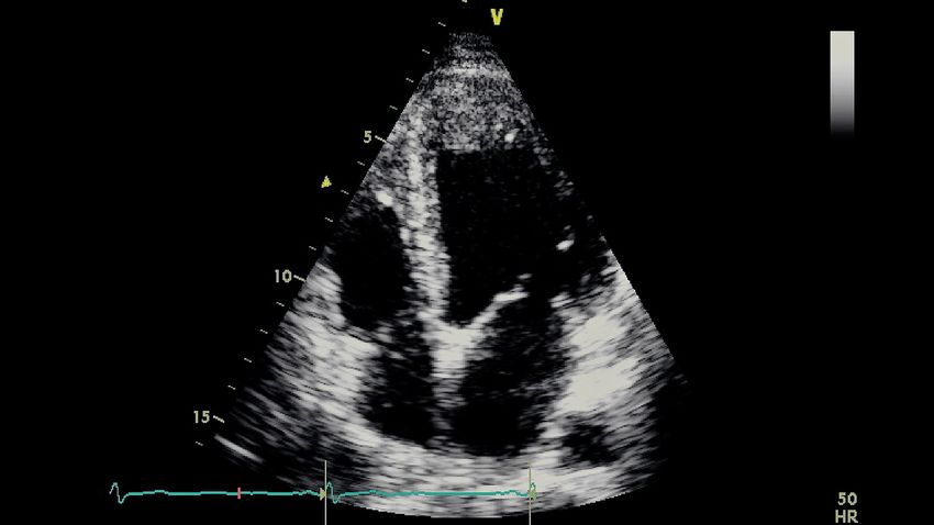
2                                                           Oumaima Hamila et al.

phy videos each acquired from a distinct patient. The 2D CNN achieved an
accuracy of 97.18% on data segmentation while the 3D CNN achieved 90.9%
of accuracy, 100% of precision and 95% of recall on MI detection. Our re-
sults demonstrate that creating a fully automated system for MI detection is
feasible and propitious.
Keywords 3D Convolutional Neural Network · Video Segmentation ·
Myocardial Infarction · Detection · Echocardiography

1 Introduction

    According to the World Health Organization, cardiovascular diseases (CVD)
are responsible for 30% of the annual mortality rate affecting roughly 18 mil-
lion humans worldwide [1, 2]. One of the prevalent cardiovascular disorders is
myocardial infarction (MI) [3] commonly referred to as heart attack. MI is
pathologically defined as the death of the myocardial cells due to extended
cardiac ischemia, which is defined as a prolonged limitation of blood supply to
the heart muscles [4]. As soon as cardiac ischemia happens, in most cases, the
patient starts showing various clinical symptoms such as chest pain, breath-
lessness or epigastric discomfort [5] which, if not treated in critical time, will
eventually lead to the death of the myocardial cells and consequently to the
death of the patient [6].
    Considering the alarming statistics revealed about MI death rates, special-
ists proclaim the urgent need to integrate machine learning (ML) and deep
learning (DL) into health-care systems to provide advanced and personalized
assistance to patients [7, 8]. Cardiovascular imaging techniques, in particular,
witnessed an evolution during the last two decades [9] which enabled cardiol-
ogists to further develop their understanding of the pathologies. Nevertheless,
studies [10, 11] show that relying on classical approaches to understanding the
data generated by cardiovascular imaging machines is insufficient and requires
modernization by integrating ML into the process of data acquisition and pro-
cessing. The tremendous ability of ML and its powerful capability of analyzing
a large quantity of data in a short time while producing results of high accuracy
and precision [12, 13], would ameliorate the diagnosis of CVD and eventually
elevate the chances of patients in receiving a more targeted and customized
treatment [14].
    Echocardiography as a cardiac imaging tool used in particular by cardiol-
ogists is highly recommended by The American Society of Echocardiography
because of its capability to assess in real-time both the cardiac function and
structure [15]. It generates important amounts of visual data including the size
and shape of the heart and its chambers and the motion of the heart walls
while they are beating, which helps cardiologists to detect MI. Studies have
shown that the occurrence of MI is highly correlated with abnormalities in
the motion of the left ventricle (LV) walls [16], known as regional wall motion
abnormalities (RWMA) of the LV [17, 18, 19]. Thus, assessing RWMA in the
LV by analyzing visual data acquired from echocardiography will help doctors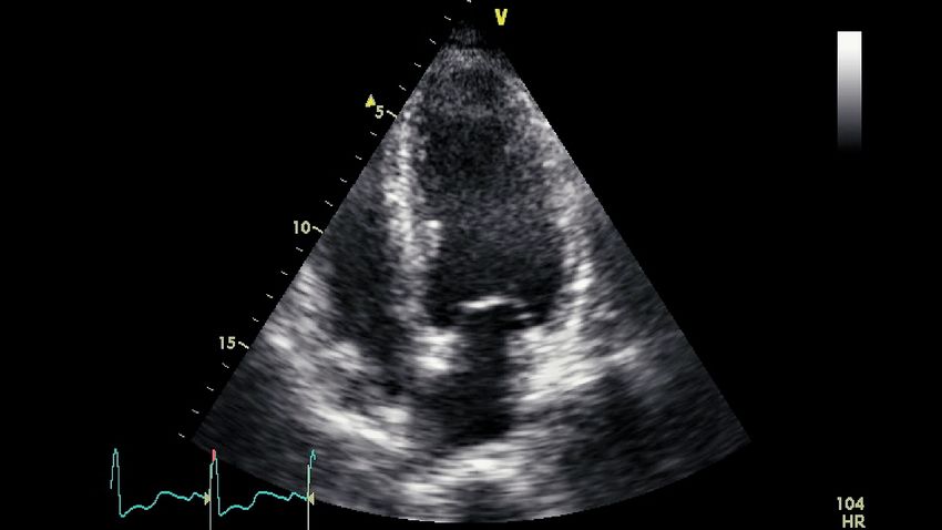
3

detect signs of MI and quickly treat the patients’ conditions [20].
    An early treatment of MI will minimize the damage on the cardiac mus-
cle tissues and prevent patients from facing fatal consequences [19]. Hence,
echocardiography is becoming indispensable to cardiologists since other bed-
side assessments are incapable of providing detailed views of the heart’s cham-
bers and walls [21]. Nonetheless, echocardiography tests produce large and
complex data that needs to be entirely exploited and understood in order to
make a complete diagnosis based on visual interpretation [7], which is highly
dependent on the level of experience of the cardiologist in question [22]. More-
over, in some cases, an important amount of the generated data remain unused
due to insufficient time and difficulty in interpretation [23]. Furthermore, data
acquisition is usually performed in emergencies, which often yields images of
low quality [24, 25]. Consequently, this significantly decreases the accuracy of
the diagnosis [26]. Therefore, cardiologists along with researchers, have been
investigating the possibility of integrating automatic programs into cardiovas-
cular imaging machines to create a more reliable diagnosis process [27, 28].
    To address some of the aforementioned issues, several approaches have
been developed in order to analyze the cardiac motion or mass. Some of which
are based on signal-processing analysis such as Fourier tracking [29], or meta-
heuristics such as genetic algorithms [30], or feature engineering [31]. Some
other works use ML and convolutional neural networks (CNN) [32, 33, 34].
However, these methods either heavily rely on very specific and limited con-
ditions of data acquisition (high-resolution echocardiograms, high frame-rate,
minimal noise) [28], or require the technician or the cardiologist to perform
preliminary preprocessing steps to be able to proceed with the prediction pro-
cess [35].
    In this paper, we propose a method to overcome the following issues: i)
subjective reading of the data that relies on expert cardiologists, ii) generated
poor-quality videos, iii) massive amounts of video preprocessing, and iv) man-
ual MI detection. Thus, the proposed solution is a fully automated pipeline
consisting of a 2D CNN that performs data preprocessing followed by a 3D
CNN that performs binary classification to detect MI from echocardiography
videos. Our proposed pipeline begins with a 2D CNN that segments the LV
region from an echocardiography video, since the occurrence of MI is strongly
dependent on signs of RWMA of the LV. Then, the segmented video is fed to
a 3D CNN, which extracts the relevant spatio-temporal features from it and
uses these features to detect the presence of MI. The input to the pipeline is
an unprocessed echocardiography acquired by a technician or a cardiologist
from a patient, and the output is the detection result. We trained our 2D and
3D CNNs using a dataset provided by Hamad Medical Corporation [36] com-
posed of 165 transthoracic echocardiograms (TTE) belonging to anonymous
patients.
    The main contribution of this work is a fully automated pipeline for video
segmentation and MI detection from echocardiography, which is also an in-
discriminative pipeline that processes videos of different sizes, different frame
rates and different resolutions. The proposed method is an end-to-end robust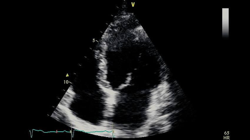
4                                                           Oumaima Hamila et al.

system that achieves 97.18% accuracy on data segmentation and 90.9% accu-
racy, 100% precision and 95% recall on MI detection. This system is robust in
that it performs well with low-quality videos corrupted with intense noise. It
is also lightweight in that it does not require high memory or computational
power in order to be executed, which makes the system adequate to be em-
bedded in external devices.
    In Section 2, we discuss existing research works related to our work. We
then explain in Section 3 the pipeline architecture and discuss details related
to the dataset. In Section 4, we explain the preprocessing techniques applied
to the dataset which is used as input to a 2D CNN. In addition, we present the
details related to the 2D CNN architecture. We describe data preprocessing
techniques applied to the processed videos before feeding it to the 3D CNN in
Section 5, together with the detials of the 3D CNN architecture. In Section 6,
we describe the training processes and the evaluation metrics related to each
model, followed by a discussion of the results. Finally, in Section 7, we present
concluding remarks.

2 Related Work

    Multiple image-processing based models that aim to evaluate the myocar-
dial motion to detect cardiovascular deficiencies have been produced over the
last few decades. In [37], a contour-based technique for detecting wall motion
abnormality by analyzing the temporal pattern of normalized wall thickening
was proposed. Epicardium and endocardium zones were manually extracted
from 14 images representing real-life patients. Subsequently, AHA 17-segment
model was used to detect regional wall changes in wall thickening with 88%
of accuracy. In [38], existing quantitative approaches were applied and tested
to identify regional LV abnormalities in patients with MI and wall motion ab-
normalities. A dataset of 4 different 2D echocardiography views and coronary
angiography was used to calculate the deviations of the contractions of the re-
gional segments of the LV wall. An abnormal segment was identified when its
deviation value is inferior to the mean contraction estimated over 10 normal
subjects. All the quantitative approaches that were evaluated achieved above
76% of accuracy.
    The second approach of processing cardiovascular data mostly uses ML
and DL algorithms. In [39], 723,754 clinically acquired Echocardiographic tests
representing 27,028 patients were acquired to predict 1-year mortality in pa-
tients who had encountered heart deficiencies. The dataset was divided into 12
groups such that each group represented a different cardiac view. Then, 12 3D
CNN models were trained separately, such that each model was trained over
one data group. The AUC values of the models ranged between 69% and 78%.
The accuracy value of the 1-year mortality prediction in patients with heart
abnormality records was 75%. [40] used DL in order to assess regional wall mo-
tion abnormality in Echocardiographic images. Data from 300 patients with a
history of MI were used and were divided into 3 groups such that each group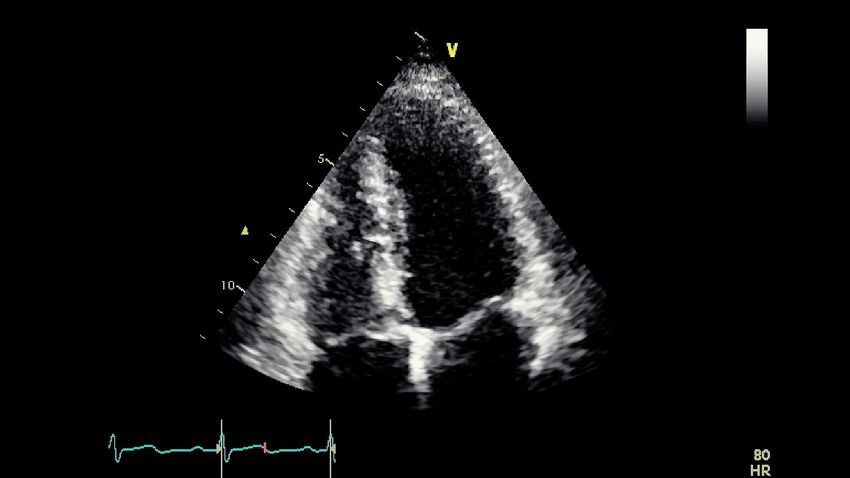
5

of data represented a specific cardiac abnormality. Data from 100 healthy pa-
tients were also added to the data groups. Then, 10 versions of the same CNN
architecture were trained and evaluated. The obtained CNN predictions were
compared with the predictions made by expert cardiologists. The AUC curve
produced by the cardiologists was similar to that produced by the CNNs (0.99
vs 0.98).
    In [41], both electrocardiogram and serum analysis were used to detect
AMI in patients who were suspected of having MI within one hour of their
arrival to the care unit. The electrical activity of the heart produced by the 12-
lead electrocardiogram was analyzed. Moreover, several chemical substances
such as creatine kinase and myoglobin were measured. These parameters were
combined to perform a logistic regression analysis that led to the detection of
MI by 64% of accuracy, and 11% of false-positive rate.

3 Methodology

    One of the main goals of our work is to create a fully automated pipeline
for LV segmentation and MI detection based on signs of RWMA of the LV
in order to assist technicians and cardiologists in the process of analyzing a
patient’s echocardiography. This system must be lightweight enough to be
easily integrated into an embedded system, and as efficient and accurate as
possible. In emergencies, for example, the data acquisition tend to be made
quickly, which may impact the echocardiography video quality. Moreover, the
majority of the echocardipgraphy machines used in hospitals produce low-
quality videos of a frame rate below 30 frames per second (fps). In the following
sections, we give an overview of the pipeline architecture and a description of
the echocardiography videos acquired for this work.

3 .1 Pipeline Overview

Figure 1 illustrates the flow of the automated pipeline where the input consists
of echocardiography video frames, and the output is the MI detection result,
MI or normal (N). The echocardiography frames are processed by the sliding
window technique which divides each frame into spatial windows of equal di-
mension. The spatial windows are passed through the 2D CNN to segment the
LV from each frame’s spatial windows. Once the segmented windows are pro-
duced, they are reassembled into segmented frames. These segmented frames
are reassembled to produce a segmented video, where the order of appear-
ance of each segmented frame is kept in the same order of appearance in the
original echocardiography video. The segmented video frames are labelled in
Figure 1 as the segmented LV from the echocardiography video frames. These
are then processed by another sliding window to produce temporal windows
of the same dimensions. The temporal windows are then passed through a 3D
CNN that classifies them into one of the two classes: abnormal (MI) or normal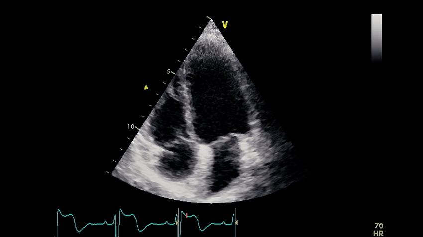
6                                                                Oumaima Hamila et al.

Fig. 1 Fully automated pipeline for MI detection, where the input is an echocardiography
video and the output is the prediction results

(N). The final class of the input video is estimated as the statistical mode of
all the predictions of the frames constituting the video.

3 .2 Echocardiography Dataset

    In collaboration with our co-authors, we have used a dataset of 165 an-
notated echocardiography videos from the study number MRC-01-19-052 ap-
proved by the Medical Research Centre at Hamad Medical Corporation. The
dataset was created by collecting various echocardiography tests from the hos-
pital’s archive. The patient’s identities remain anonymous. The tests represent
the A4C view, and have a frame rate of 25 fps. The prevalent problem during
data collection was the corruption of videos due to either noise or distorted
representation of the A4C view, which usually consists of missing parts of the
heart chambers that failed to be acquired during the echocardiography test.
In this work, our dataset included both poor and good quality videos.
    In accordance with the definition of MI abnormalities as stated in [4], this
work focuses on learning RWMA of the LV chamber to detect MI from the
A4C view. Figure 2 shows a captured frame representing the A4C view from
our dataset, which consists of four distinct heart chambers, numbered from 1
to 4, where 1 identifies the LV, 2 to 4 identifies the Right Ventricle, the Left
Atrium, and the Right Atrium, respectively.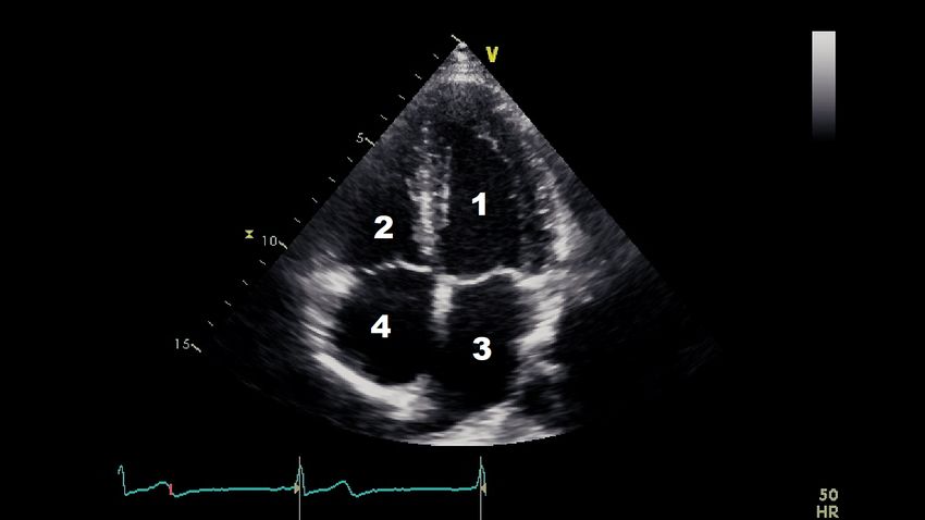
7
Fig. 2 Apical four-chamber view. The numbers from 1 to 4 marking the four different
chambers correspond respectively to the LV, the right ventricle, the left atrium, and the
right atrium
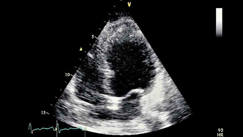
Figure 3 represents captured frames representing the quality of several
videos from our dataset, which varies from good to noisy. Figures from 3a to
3f correspond to distinct frames each captured from different videos. We notice
that in Figure 3a the left wall of the LV is blurred. Also, in Figure 3b, the left
wall of the LV is blurred and almost missing. In the same way, we observe that
the totality of the LV wall is blurred in Figure 3c; and that the interior of the
LV is disrupted with noise in Figure 3d. Finally, both Figure 3e and Figure 3f
show acceptable LV representations, where the LV walls are captured and the
chamber’s interior is empty from noise. Moreover, since our study is centered
on the LV chamber only, we purposely ignore the distortions of the rest of
the cardiac chambers (Right Ventricle, Left Atrium, and Right Atrium) in the
dataset videos. For example, in Figure 3e, both the Left Atrium and the Right
Atrium are partially cut from the view, however, this does not impact our
study.
Hence, our final set of videos for segmentation consists of both clear and
blurred video images of the LV chamber.
4 Video Segmentation with 2D CNN
The 2D CNN performs a supervised classification by learning to map the
input echocardiography video to its adequate segmentation mask. Thus, we
manually created segmentation masks that cover the LV chamber from the
A4C view and discards the remaining chambers. The manually created seg-
mentation masks were assigned to the dataset video frames as labels, and fed8 Oumaima Hamila et al.
(a) (b)
(c) (d)
(e) (f )
Fig. 3 Captured frames from 6 different videos of our dataset, where each image from 3a to
3f corresponds to a distinct video. 3a represents a blurred left wall in the LV, 3b represents
a missing left wall in the LV, 3c represents blurred LV walls, 3d represents noise inside the
LV, and 3e and 3f represent normal echocardiograms
to the 2D CNN to learn the best segmentation mask from any given echocar-
diography video. The videos were normalized prior to training the 2D CNN
by means of the sliding window technique due to differences in the dimensions
of the frames.
4 .1 Data Preprocessing for 2D CNN
4 .1.1 Creating labels
The first step was preparing a labeled dataset, where each input is an
echocardiography video frame, and each output is a corresponding segmen-
tation mask. The segmentation masks were manually created and designed
to cover the area of LV from the A4C in all the frames included in a given9
video. In each video, at least one cardiac cycle was performed, which means
that we have at least one diastole (when the heart refills with blood) and one
systole (when the heart pumps the blood) per video. The segmentation mask
boundaries were determined such that they form a rectangle that encompasses
the totality of the LV even on the frames where the heart is fully expanded,
i.e. during diastole when the LV reaches its maximum volume. We assigned
one segmentation mask for each echocardiography video. Consequently, the
segmentation mask assigned to a video was the same assigned to each of its
frames. Thus, the final dataset that was used to train the 2D CNN contained
the video frames as the input samples, and the segmentation masks as the
labels or the output samples.
4 .1.2 Spatial windowing: segmentation process
The next step was to produce frames of the same spatial dimensions (frame
size). Thereby, we opted for the sliding window technique to create spatial
windows of fixed dimensions, and we applied the technique on both the input
samples and the labels. The technique consists of extracting consecutive win-
dows of equal dimensions with an overlap between two successive windows.
Normally, the dimension of the window must be less than or equal to the orig-
inal dimension of the frame from which it was extracted. Also, the overlap
should be less than the dimension of the window. In Figure 4, we illustrate the
sliding window technique, where it extracts two successive windows with an
overlap equal to 50%. The red square in the figure represents a window and
the green square represents its successive window that overlaps with the red
square by 50%.
By applying the sliding window technique on the dataset, we created win-
dows of dimension equal to 150 × 150 pixels (px), with a 50% spatial overlap
equal to 75 px. The dimensions of the windows are always less than the origi-
nal dimensions of the video frames, where the smallest frame dimension in the
input samples is equal to 422 × 636 px. In this manner, we uniformized and
increased the input samples by producing a total of 108,127 windows.
The 2D CNN generates an estimation of a segmentation mask for an input
window where each value within the segmentation mask is in the interval
[0, 1]. We round these values to obtain a perfect mask with pixel values equal
to either 0 or 1. Once the segmentation mask corresponding to each window is
estimated, the complete segmentation mask of a video frame is reconstructed
using the inverse sliding window technique. The technique is performed by
adding the successive estimated segmentation masks of every window from a
certain frame with an overlap equal to 50% until we recover the entire frame.
The reconstructed frame has the same dimension as the original frame cut
from its video. With the same inverse sliding window technique, we recover
all the segmentation video frames and also all the segmentation masks, where
each mask corresponds to a frame. Then, having all the segmentation masks
predicted for each frame of a given video, we aggregate these masks employing10 Oumaima Hamila et al.
Fig. 4 Sliding window: the process of extracting two consecutive spatial windows from an
frame with an overlap equal to 50% between the successive windows
statistical mode (i.e. the most represented value in each pixel is chosen) to
form the segmentation mask corresponding to the totality of a video.
Figure 5 encapsulates the process of applying the predicted segmentation
mask on a video frame. Figure 5a shows an original video frame, while Figure
5b shows its corresponding predicted mask recovered from the reverse sliding
window technique, which appears as a set of points with undefined bound-
aries. Hence, to recover a rectangular-shaped segmentation mask we apply
the minimum bounding box technique to enclose the estimated set of points
into a rectangle and to produce a bounding box as shown in Figure 5c. Then,
each video frame is multiplied by its corresponding bounding box to produce
a segmented frame as shown in Figure 5d. The segmented frames belonging
to the same video are then reassembled to produce a segmented video, where
the order of appearance of each segmented frame is kept in its same order of
appearance as in the original video. The segmented video has the same num-
ber of frames as the original video prior to any preprocessing, however, it has
inferior frame sizes.
4 .2 2D CNN Architecture
Our 2D CNN architecture follows the encoder-decoder design common to
CNNs developed for semantic segmentation problems [42, 43, 44]. Figure 6 illus-
trates the detailed configuration of the 2D CNN consisting of 3 convolutional
layers with rectified linear unit (ReLU) as the activation function for each
layer. Every convolutional layer is followed by a max-pooling layer to reduce
the dimension of the window. Then, the convolutional layers are followed by
3 transpose convolutional layers [45] with a stride equal to 2 × 2 in order to
reacquire the initial input dimension. Each transpose layer uses a ReLU as its
activation function. The last layer is a convolutional layer with a sigmoid acti-
vation function, which was selected to produce a predicted segmentation mask11
(a) (b)
(c) (d)
Fig. 5 Captured images from the different stages of the segmentation mask process applied
to a video frame, where 5a represents the original video frame. 5b represents the segmenta-
tion mask corresponding to the frame (a) and obtained from the 2D CNN. 5c corresponds
to the minimum bounding box of the predicted segmentation mask in 5b, and 5d is the
segmented frame resulted from multiplying the original video frame 5a by the minimum
bounding box in 5c
with pixel values equal to probabilities between the range of [0, 1]. The input
and output dimensions are 150 × 150 px, which correspond to a segmentation
mask adequate for the input window.
5 MI Detection with 3D CNN
In this section, we detail the proposed MI detection using a 3D CNN over
the segmented echocardiography videos obtained from a 2D CNN. However,
these segmented videos have a different number of frames and different di-
mensions. In the following section, we give preprocessing details of segmented
videos.
5 .1 Data Preprocessing with 3D CNN
To solve the issue of differences in the spatial dimensions, all the video
frames were scaled down to the smallest video size in the dataset. In our case,12 Oumaima Hamila et al.
Fig. 6 The architecture of the 2D CNN
the smallest frame size from the segmented videos is equal to 236 × 183 px.
Then, we applied the sliding window technique to the resized videos in order
to obtain a uniform number of frames. The technique consists of extracting a
temporal window created from a consecutive number of frames from a given
video and repeating the process by going over all the video frames with respect
to an overlap between two successive temporal windows. In general, the over-
lap size is inferior to the temporal window size. The technique allows dividing
the dataset videos into smaller temporal windows of a fixed number of frames.
It also allowed us to increase the number of samples for the 3D CNN from
165 segmented videos to 2000 temporal windows. In our case, we applied the
sliding window technique to extract temporal windows of size equal to 5, 7,
and 9 frames per window, with an overlap equal respectively to 4, 6, and 8
frames (i.e. the sliding window moves forward by one window per step). By
varying the size of the temporal windows, we created 3 different datasets that
we used to train 3 different 3D CNN models.
We illustrate in Figure 7 the sliding window technique for a temporal win-
dow size equal to 5. The red window represents a temporal window consisting
of 5 successive frames. The green window is the successive temporal window
of the red one that also contains 5 frames, such that the first 4 frames from
the green window are the same as the last 4 frames from the red window. The
labels attributed to these temporal windows are the same as the labels of the
video from which these windows were extracted.
Table 1 shows the number of the temporal windows obtained from the
dataset videos by varying the frame number of the temporal windows. For a13
Fig. 7 Temporal sliding window depicting the process of extracting 2 consecutive temporal
windows of size 5 frames, with an overlap equal to 4 frames between two consecutive windows
window size equal to 5, 7 and 9, we obtained respectively 2841, 2511, and 2181
temporal windows from the dataset of the segmented videos.
Table 1 Number of windows obtained by applying the temporal sliding window technique
with different window sizes
Size of the temporal window Number of windows
5 frames 2841
7 frames 2511
9 frames 2181
In another experiment, we applied a sliding window technique that extracts
spatio-temporal windows from the segmented videos in an attempt to avoid
rescaling the videos to the smallest dimension. The technique consists of com-
bining the temporal and spatial sliding window techniques at the same time.
Even though this process resulted in a larger dataset, the predicted accuracies
were lower than those obtained by simply resizing the segmented videos and
applying only temporal sliding window. Therefore, we concluded that the LV
chamber should be fully preserved as a frame in the echocardiography video
for the 3D CNN to capture all the details throughout the process of learning.
Cutting the LV chamber from a segmented video by a spatial sliding window
will deteriorate the information and will result in a poor model.14 Oumaima Hamila et al.
5 .2 3D CNN Architectures
In this section, we present the architectures of the 3D CNN models used
to train the 3 datasets separately. For each dataset, we used the same model
architecture: same number of layers, the same number of neurons and same
activation functions. However, we changed the kernel size for each model to
make it fit with the input dimension of the windows.
Figure 8 shows the architecture of the 3D CNN consisting of 4 3D convo-
lutional layers, 4 2D max-pooling layers, and 3 dense layers. The activation
function used for all the layers, both convolutional and dense, except for the
output layer, is ReLU. For the output layer, which consists of one neuron that
contains the prediction probability, we used the sigmoid activation function.
Table 2 gives the details of the characteristics of each 3D CNN model.
Fig. 8 The generic architecture of the 3D CNN used to train all the datasets
6 Experiments and Results
6 .1 2D CNN: Training and Evaluation Metrics
In order to train the 2D CNN for the task of predicting segmentation
masks, we normalized the data to values in the interval [0, 1]. Then, we di-
vided the dataset into disjoint subsets for training and testing, consisting of
80% and 20% of the dataset, respectively. Next, we create a sub-set for the
validation set, to fine-tune the hyper-parameters of the model, equal to 20%
of the 80% of the training set. We trained the model for 100 epochs with a15
Table 2 3D CNN characteristics per layer according to the size of the temporal window
Kernel size per window size
Layer No. of neurons 5 7 9
Conv3D 32 (3, 3, 3) (3, 3, 3) (3, 3, 3)
MaxPooling - (2, 2, 1) (2, 2, 1) (2, 2, 1)
Conv3D 32 (3, 3, 2) (3, 3, 3) (3, 3, 3)
MaxPooling - (2, 2, 1) (2, 2, 1) (2, 2, 1)
Conv3D 16 (3, 3, 2) (3, 3, 2) (3, 3, 3)
MaxPooling - (2, 2, 1) (2, 2, 1) (2, 2, 1)
Conv3D 8 (3, 3, 1) (3, 3, 2) (3, 3, 3)
MaxPooling - (2, 2, 1) (2, 2, 1) (2, 2, 1)
Flatten -
Dense 32
Dense 16
Dense 1
batch size equal to 256. The total trainable parameters of the 2D CNN are
equal to 192,617. We used the sigmoid activation function for the last layer,
and RMSProp optimizer as the optimization function for the 2D CNN. To
evaluate the model’s performance we used the mean squared error (MSE) as
the loss function. As a result, the MSE is defined as
wXh −1 wX
w −1
1
M SE(w, ŵ) = [w(i,j) − ŵ(i,j) ]2 . (1)
wh ww i=0 j=0
In Eq. 1, wh and ww are the window’s height and width, respectively, while
w and ŵ are the actual window and its corresponding prediction, respectively.
All relevant details regarding the training parameters of the 2D CNN are
presented in Table 3.
Table 3 2D CNN training parameters
Parameters Values
Input samples (windows) 86, 502 (80%)
Input shape (150, 150)
Output shape (150, 150)
Trainable parameters 192, 617
Loss MSE
Optimizer RMSProp
Epochs 100
Batch size 25616 Oumaima Hamila et al.
6 .2 2D CNN: Results and Discussion
We evaluated the model using the test set by calculating the accuracy as
Accuracy(w, ŵ) = 1 − M SE(w, ŵ). (2)
The model achieved 97.18% accuracy over the test set, which implies that ex-
tracting the LV region manually can be replaced by an automatic segmentation
method of high precision.
6 .3 3D CNNs: Training and Evaluation Metrics
For the 3D CNN experiments, we split the dataset into training and test
sets consisting of 80% and 20% of the dataset, respectively. Since MI detec-
tion is a binary classification, we ensured that the dataset is balanced with
respect to N and MI classes. Then, we applied 5-fold cross-validation (CV)
[46] on each 3D CNN model. We evaluated the trained models using their
corresponding test sets. However, our goal is to predict the class of a complete
echocardiography video rather than the class of a temporal window. Thus, to
calculate the evaluation metrics of the 3D model over the task of MI detec-
tion per video, we assigned a prediction class to each video as the result of
the statistical mode calculated over all the predicted classes of the windows
constituting that video.
The evaluation metrics used to assess the performance of the models are
as follows:
TP
P = ,
TP + FP
TP
R= , and (3)
TP + FN
2×P ×R
F1 = ,
P +R
where P, R, and F1 are Precision, Recall and F1 score respectively, while TP,
FP, and FN are True Positive, False Positive and False Negative respectively.
To train the models, we used the same loss function, learning rate, and
optimizer, however, the input shape varies between the models as shown in
Table 4. We used binary cross-entropy as the loss function [47], and the RM-
SProp optimizer with a learning rate equal to 1e−3 . For each fold, we trained
the model for 100 epochs using a batch size equal to 8 samples. We calculated
the evaluation metrics per video for each fold associated with each model.
To implement the 3D CNN models, we used the Python programming
language and its open-source neural network library Keras [48]. We run the
experiments on an NVIDIA Tesla P100 GPU server with 12GB of GPU mem-
ory.17
Table 4 3D CNN models’ training parameters per window size
Window size
Parameters 5 7 9
Input samples (windows) 2273 2009 1745
Input shape (236,183,5) (236,183,7) (236,183,9)
Trainable parameters 57, 977 68, 345 74, 105
Loss Binary CrossEntropy
Optimizer RMSProp
Learning rate 1e−3
Epochs per fold 100
Batch size 8
6 .4 3D CNNs: Results and Discussion
Table 5 shows the results of the evaluation metrics, as produced by the fully
trained 3D models using 5-fold CV and calculated with their corresponding
test sets. Only the highest, lowest, and mean values are given.
The best results of our models were 90.9% of accuracy, 97.2% F1 score,
100% precision, and 95% recall. However, the mean values for the evaluation
metrics are slightly lower than the maximum values, and this is explained by
the fact that the training sets contain distinct training samples, where some
of the windows contain more noise and hence are of poorer quality than other
windows. Therefore, even though all the sets contain balanced and equal pro-
portions of samples representing both classification classes, some of the folds
may contain more noisy samples than the remaining folds, which influences
the learning performance of the model at each fold. Hence, the model trained
over the dataset of windows with the size equal to 5 frames, achieved 84.6% as
the mean accuracy over the 5 folds of the CV, 87% as the mean value of the
F1 score, 89% precision, and 85.1% the mean value of the recall. Furthermore,
we observe that the mean values of the evaluation metrics obtained from the
dataset of windows equal to 7 frames are slightly inferior to those attained from
the dataset of windows with a size equal to 5. Likewise, the mean values of the
evaluation metrics achieved over the dataset of windows equal to 9 frames, are
less than those obtained over the windows of size equal to 7 frames. The mean
values of the metrics obtained from the second dataset (window size 7) are
respectively equal to 82.5% of accuracy, 83.2% of F1 score, 83.5% of precision
and 83.1% of recall, whereas, the values obtained from the third (window size
9) are respectively equal to 81.3% of accuracy, 83.1% of F1 score, 84.6% of
precision and 82% of recall. Thus, we conclude that enlarging the size of the
temporal window reduces the performance of the 3D CNN.
7 Conclusion and Future Work
In this paper, we proposed a novel, real-time, and fully automated ap-
proach based on 2D and 3D CNN models to detect MI from the echocar-18 Oumaima Hamila et al.
Table 5 3D CNN models’ evaluation metrics per window size
Window size
Evaluation metrics 5 7 9
Max 90.3 % 90.9 % 90.0 %
Accuracy Mean 84.6 % 82.5 % 81.3 %
Min 77.1 % 72.9 % 68.4 %
Max 94.8 % 97.2 % 92.3 %
F1 score Mean 87.0 % 83.2 % 83.1 %
Min 68.7 % 75.0 % 68.4 %
Max 94.7 % 100 % 94.7 %
Precision Mean 89.0 % 83.5 % 84.6 %
Min 73.0 % 75.0 % 72.2 %
Max 95.0 % 94.7 % 90.0 %
Recall Mean 85.1 % 83.1 % 82.0 %
Min 65.0 % 75.0 % 65.0 %
diography of a patient. This approach replaces the time-consuming manual
preprocessing with a fast and reliable LV segmentation; and improves MI de-
tection by accurate MI-prediction results in real-time. The proposed 2D CNN
model for video segmentation achieved a high accuracy of 97.18% in segment-
ing LV from the A4C, thus showing that it could be very reliable and valuable
to cardiologists. Moreover, the proposed 3D CNN models demonstrated that
real-time prediction of MI from a patient’s echocardiography is feasible and
efficient. It achieved 90.9% accuracy, 100% precision, 95% recall, and 97.2%
F1 score. We believe that noisy and low-quality echocardiography deteriorated
the MI detection performance of the 3D CNN models from the segmented LV
views. Nevertheless, the results demonstrate the robustness and efficiency of
the proposed approach, which was able to detect MI regardless of the quality.
Accuracy, precision, recall as well as F1 score vary depending on the tempo-
ral window size. We relate this variability to the difference in the 3D CNN
model’s characteristics, which may alter the ability of the model to extract
relevant prediction features with the given neuron and layer parameters. The
3D CNN models were built with the objective of assigning a few layers and
neurons that are able to extract relevant spatio-temporal features from the
temporal windows without focusing on irrelevant details that would decrease
the prediction accuracy. For our future work, we aim to merge our end-to-end
automated pipeline into an embedded system using TensorRT [49]. In addi-
tion, we aspire to improve our model’s results by enlarging the dataset with
more echocardiography videos [50].
Acknowledgements
The authors wish to acknowledge the valuable contribution of researchers
at Medical Research Centre at Hamad Medical Corporation in the State of
Qatar for the creation of this work and this publication.19
Declarations
Funding
The work of Sheela Ramanna and Christopher J. Henry was funded by the
NSERC Discovery Grants Program (nos. 194376, 418413).
Conflicts of interest/Competing interests
There is no conflict of interest with the funders.
Consent to participate
All the Authors consent to the content of the manuscript.
References
1. Lawrence J. Laslett, Peter Alagona, Bernard A. Clark, Joseph P. Drozda, Frances Sal-
divar, Sean R. Wilson, Chris Poe, and Menolly Hart. The worldwide environment of
cardiovascular disease: Prevalence, diagnosis, therapy, and policy issues. Journal of the
American College of Cardiology, 60(25 Supplement):S1–S49, 2012.
2. World Health Organization cardiovascular diseases. https://www.who.int/en/
news-room/fact-sheets/detail/cardiovascular-diseases-(cvds). Accessed: 2020-
09-14.
3. MD FESC Lüscher, Thomas F. Myocardial infarction: mechanisms, diagnosis, and
complications. European Heart Journal, 36(16):947–949, 04 2015.
4. Kristian Thygesen, Joseph S. Alpert, Allan S. Jaffe, Bernard R. Chaitman, Jeroen J.
Bax, David A. Morrow, and Harvey D. White. Fourth universal definition of myocardial
infarction (2018). volume 72, pages 2231–2264. Journal of the American College of
Cardiology, 2018.
5. Lei Lu, Min Liu, RongRong Sun, Yi Zheng, and Peiying Zhang. Myocardial infarction:
Symptoms and treatments. Cell Biochemistry and Biophysics, 72, 07 2015.
6. Frans Van de Werf, Diego Ardissino, Dennis V Cokkinos, Keith A A Fox, Desmond
Julian, and et. al. Management of acute myocardial infarction in patients presenting
with st-segment elevation. European heart journal, 24:28–66, 01 2003.
7. Nestor Gahungu, Robert Trueick, Saiuj Bhat, Partho P. Sengupta, and Girish Dwivedi.
Current challenges and recent updates in artificial intelligence and echocardiography.
Current Cardiovascular Imaging Reports, 13(2), Feb 2020.
8. Thomas Davenport, Ravi Kalakota, and Dennis V Cokkinos. The potential for artificial
intelligence in healthcare. Future healthcare journal, 6(2):94–98, 06 2019.
9. Girish Dwivedi, Kwan L. Chan, Matthias G. Friedrich, and Rob S.B. Beanlands. Car-
diovascular imaging: New directions in an evolving landscape. Canadian Journal of
Cardiology, 29(3):257 – 259, 2013.
10. Jeroen Bax and Victoria delgado. Advanced imaging in valvular heart disease. Nature
Reviews Cardiology, 14, 01 2017.
11. Pamela S. Douglas, Manuel D. Cerqueira, Daniel S. Berman, Kavitha Chinnaiyan,
Meryl S. Cohen, Justin B. Lundbye, and et al. The future of cardiac imaging: Report
of a think tank convened by the american college of cardiology. JACC: Cardiovascular
Imaging, 9(10):1211 – 1223, 2016.20 Oumaima Hamila et al.
12. Chensi Cao, Feng Liu, Hai Tan, Deshou Song, Wenjie Shu, Weizhong Li, Yiming Zhou,
Xiaochen Bo, and Zhi Xie. Deep learning and its applications in biomedicine. Genomics,
Proteomics & Bioinformatics, 16, 03 2018.
13. Morgan P. McBee, Omer A. Awan, Andrew T. Colucci, Comeron W. Ghobadi, Nadja
Kadom, Akash P. Kansagra, Srini Tridandapani, and William F. Auffermann. Deep
learning in radiology. Academic Radiology, 25(11):1472 – 1480, 2018.
14. Rahul Kumar Sevakula, Wan-Tai M. Au-Yeung, Jagmeet P. Singh, E. Kevin Heist,
Eric M. Isselbacher, and Antonis A. Armoundas. State-of-the-art machine learning
techniques aiming to improve patient outcomes pertaining to the cardiovascular system.
Journal of the American Heart Association, 9(4):e013924, 2020.
15. John S. Gottdiener, James Bednarz, Richard Devereux, Julius Gardin, Allan Klein,
Warren J. Manning, Annitta Morehead, Dalane Kitzman, Jae Oh, Miguel Quinones,
Nelson B. Schiller, James H. Stein, and Neil J. Weissman. American society of echocar-
diography recommendations for use of echocardiography in clinical trials. Journal of
the American Society of Echocardiography”, issn = ”0894-7317, 17(10):1086–1119, oct
2004.
16. Ioanna Kosmidou, Björn Redfors, Harry P. Selker, Holger Thiele, Manesh R. Patel,
James E. Udelson, and et al. Infarct size, left ventricular function, and prognosis
in women compared to men after primary percutaneous coronary intervention in st-
segment elevation myocardial infarction. European Heart Journal, 38(21):1656–1663,
04 2017.
17. Adrian F. Hernandez, Eric J. Velazquez, Scott D. Solomon, Rakhi Kilaru, Rafael Diaz,
Christopher M. O’Connor, George Ertl, Aldo P. Maggioni, Jean-Lucien Rouleau, Wiek
van Gilst, Marc A. Pfeffer, and Robert M. Califf. Left Ventricular Assessment in Myocar-
dial Infarction: The VALIANT Registry. Archives of Internal Medicine, 165(18):2162–
2169, 10 2005.
18. Vittorio Palmieri, Peter M. Okin, Jonathan N. Bella, Eva Gerdts, Kristian Wachtell,
Julius Gardin, Vasilios Papademetriou, Markku S. Nieminen, Björn Dahlöf, and
Richard B. Devereux. Echocardiographic wall motion abnormalities in hypertensive pa-
tients with electrocardiographic left ventricular hypertrophy. Hypertension, 41(1):75–82,
2003.
19. Serkan Kiranyaz, Aysen Degerli, Tahir Hamid, Rashid Mazhar, Rayyan Ahmed, Rayaan
Abouhasera, Morteza Zabihi, Junaid Malik, Hamila Ridha, and Moncef Gabbouj. Left
ventricular wall motion estimation by active polynomials for acute myocardial infarction
detection. 08 2020.
20. R S Horowitz, J Morganroth, C Parrotto, C C Chen, J Soffer, and F J Pauletto. Im-
mediate diagnosis of acute myocardial infarction by two-dimensional echocardiography.
Circulation, 65(2):323–329, 1982.
21. Jonathan Gaudet, Jason Waechter, Kevin McLaughlin, André Ferland, Tomás Godinez,
Colin Bands, Paul Boucher, and Jocelyn Lockyer. Focused critical care echocardiogra-
phy. Critical Care Medicine, 44:1, 06 2016.
22. Joseph E. O’Boyle, Alfred F. Parisi, Markku Nieminen, Robert A. Kloner, and Shukri
Khuri. Quantitative detection of regional left ventricular contraction abnormalities by
2-dimensional echocardiography. The American Journal of Cardiology, 51(10):1732 –
1738, 1983.
23. Gill Wharton, Richard Steeds, Bushra Rana, Richard Wheeler, Smith N, David Oxbor-
ough, Brewerton H, Jane Allen, Chambers J, Julie Sandoval, Guy Lloyd, Prathap Kana-
gala, Matthew T, Massani N, and Richard Jones. A minimum dataset for a standard
transthoracic echocardiogram, from the british society of echocardiography education
committee. Echo Research and Practice, 2, 03 2015.
24. Mustafa Kurt, Kamran Shaikh, Leif Peterson, Karla Kurrelmeyer, Gopi Shah, Sherif
Nagueh, Robert Fromm, Miguel Quinones, and William Zoghbi. Impact of contrast
echocardiography on evaluation of ventricular function and clinical management in a
large prospective cohort. Journal of the American College of Cardiology, 53:802–10, 03
2009.
25. Aleksandar N. Neskovic, Andreas Hagendorff, Patrizio Lancellotti, Fabio Guarracino,
Albert Varga, Bernard Cosyns, Frank A. Flachskampf, Bogdan A. Popescu, and et al.
Emergency echocardiography: the European Association of Cardiovascular Imaging rec-
ommendations. European Heart Journal - Cardiovascular Imaging, 14(1):1–11, 01 2013.21
26. Y. Nagata, Yuichiro Kado, Takeshi Onoue, K. Otani, Akemi Nakazono, Y. Otsuji, and
M. Takeuchi. Impact of image quality on reliability of the measurements of left ven-
tricular systolic function and global longitudinal strain in 2d echocardiography. Echo
Research and Practice, 5:27 – 39, 2018.
27. Maleeha Qazi, Glenn Fung, Sriram Krishnan, Romer Rosales, Harald Steck, R. Bharat
Rao, Don Poldermans, and Dhanalakshmi Chandrasekaran. Automated heart wall
motion abnormality detection from ultrasound images using bayesian networks. page
519–525, 2007.
28. Chieh Chen Wu, Wen Ding Hsu, Md Mohaimenul Islam, Tahmina Nasrin Poly, Hsuan
Chia Yang, Phung Anh (Alex) Nguyen, Yao Chin Wang, and Yu Chuan (Jack) Li. An
artificial intelligence approach to early predict non-st-elevation myocardial infarction
patients with chest pain. Computer Methods and Programs in Biomedicine, 173:109–
117, may 2019.
29. Yudong Zhu, Maria Drangova, and Norbert J. Pelc. Fourier tracking of myocardial
motion using cine-pc data. Magnetic Resonance in Medicine, 35(4):471–480, 1996.
30. Abhishek Mishra, Pranab Dutta, and M.K. Ghosh. A ga based approach for boundary
detection of left ventricle with echocardiographic image sequences. Image and Vision
Computing, 21:967–976, 10 2003.
31. Aysen Degerli, Morteza Zabihi, Serkan Kiranyaz, Tahir Hamid, Rashid Mazhar, Hamila
Ridha, and Moncef Gabbouj. Early detection of myocardial infarction in low-quality
echocardiography. 10 2020.
32. Mingqiang Chen, Lin Fang, Qi Zhuang, and Huafeng Liu. Deep learning assessment of
myocardial infarction from mr image sequences. IEEE Access, PP:1–1, 01 2019.
33. Sukrit Narula, Khader Shameer, Alaa Mabrouk Salem Omar, Joel T. Dudley, and
Partho P. Sengupta. Machine-learning algorithms to automate morphological and func-
tional assessments in 2d echocardiography. Journal of the American College of Cardi-
ology, 68(21):2287–2295, 2016.
34. Serkan Kiranyaz, Morteza Zabihi, Ali Bahrami Rad, Turker Ince, Ridha Hamila, and
Moncef Gabbouj. Real-time phonocardiogram anomaly detection by adaptive 1d con-
volutional neural networks. Neurocomputing, 411:291–301, 2020.
35. K. E. T. Upendra, G. A. C. Ranaweera, N. H. A. P. Samaradiwakara, A. Munasinghe,
K. L. Jayaratne, and M. I. E. Wickramasinghe. Artificial neural network application in
classifying the left ventricular function of the human heart using echocardiography. In
2018 National Information Technology Conference (NITC), pages 1–6, 2018.
36. Hamad medical corporation. https://www.hamad.qa/EN/Pages/default.aspx. Ac-
cessed: 2020-09-24.
37. Mai Wael, El-Sayed Ibrahim, and Ahmed S. Fahmy. Detection of lv function abnor-
mality using temporal patterns of normalized wall thickness. Journal of Cardiovascular
Magnetic Resonance, 17:47, 02 2015.
38. P F Moynihan, A F Parisi, and C L Feldman. Quantitative detection of regional left
ventricular contraction abnormalities by two-dimensional echocardiography. i. analysis
of methods. Circulation, 63(4):752–760, 1981.
39. Alvaro Ulloa, Linyuan Jing, Christopher W. Good, David P. vanMaanen, Sushravya
Raghunath, Jonathan D. Suever, and et al. A deep neural network predicts survival
after heart imaging better than cardiologists. CoRR, abs/1811.10553, 2018.
40. Kenya Kusunose, Takashi Abe, Akihiro Haga, Daiju Fukuda, Hirotsugu Yamada, Masa-
fumi Harada, and Masataka Sata. A deep learning approach for assessment of regional
wall motion abnormality from echocardiographic images. JACC: Cardiovascular Imag-
ing, 13, 05 2019.
41. E. M. Ohman, C. Casey, J. R. Bengtson, D. Pryor, W. Tormey, and J. H. Horgan. Early
detection of acute myocardial infarction: additional diagnostic information from serum
concentrations of myoglobin in patients without st elevation. British heart journal,
163(6):335–338, 05 1990.
42. V. Badrinarayanan, A. Kendall, and R. Cipolla. Segnet: A deep convolutional encoder-
decoder architecture for image segmentation. IEEE Transactions on Pattern Analysis
and Machine Intelligence, 39(12):2481–2495, 2017.
43. Yongfeng Xing, Luo Zhong, and Xian Zhong. An encoder-decoder network based fcn
architecture for semantic segmentation. Wireless Communications and Mobile Com-
puting, 2020:1–9, 07 2020.22 Oumaima Hamila et al.
44. Victor Alhassan, Christopher J. Henry, Sheela Ramanna, and Christopher Storie. A deep
learning framework for land-use/land-cover mapping and analysis using multispectral
satellite imagery. Neural Computing and Applications, 32, 06 2020.
45. Vincent Dumoulin and Francesco Visin. A guide to convolution arithmetic for deep
learning. pages 18–23, 03 2016.
46. Payam Refaeilzadeh, Lei Tang, and Huan Liu. Cross-validation. pages 532–538, 2009.
47. Shie Mannor, Dori Peleg, and Reuven Rubinstein. The cross entropy method for clas-
sification. pages 561–568, 01 2005.
48. François Chollet et al. Keras. https://keras.io, 2015.
49. TensorRT cardiovascular diseases. https://developer.nvidia.com/
tensorrt-getting-started. Accessed: 2021-02-16.
50. Ali Madani, Jia Ong, Anshul Tibrewal, and Mohammad Mofrad. Deep echocardiog-
raphy: data-efficient supervised and semi-supervised deep learning towards automated
diagnosis of cardiac disease. npj Digital Medicine, 1, 12 2018.You can also read