Functional Maps Representation on Product Manifolds - arXiv
←
→
Page content transcription
If your browser does not render page correctly, please read the page content below
Volume xx (200y), Number z, pp. 1–10

                                                        Functional Maps Representation on Product Manifolds

                                                                   E. Rodolà1 Z. Lähner2 A. M. Bronstein3,6 M. M. Bronstein4,5,6 J. Solomon7
                                                    rodola@di.uniroma1.it laehner@in.tum.de bron@cs.technion.ac.il bronstein@imperial.ac.uk jsolomon@mit.edu
                                                       1 Sapienza   University of Rome   2 TU   Munich   3 Technion   4 USI   Lugano   5 Imperial   College London   6 Intel   7 MIT
arXiv:1809.10940v2 [cs.GR] 9 Jan 2019

                                                Abstract
                                                We consider the tasks of representing, analyzing and manipulating maps between shapes. We model maps as densities over
                                                the product manifold of the input shapes; these densities can be treated as scalar functions and therefore are manipulable
                                                using the language of signal processing on manifolds. Being a manifold itself, the product space endows the set of maps with a
                                                geometry of its own, which we exploit to define map operations in the spectral domain; we also derive relationships with other
                                                existing representations (soft maps and functional maps). To apply these ideas in practice, we discretize product manifolds
                                                and their Laplace–Beltrami operators, and we introduce localized spectral analysis of the product manifold as a novel tool
                                                for map processing. Our framework applies to maps defined between and across 2D and 3D shapes without requiring special
                                                adjustment, and it can be implemented efficiently with simple operations on sparse matrices.
                                                Keywords: shape matching, functional maps, product manifolds
                                                Categories and Subject Descriptors (according to ACM CCS): I.3.5 [Computer Graphics]: Computational Geometry and Object
                                                Modeling—Shape Analysis, 3D Shape Matching, Geometric Modeling

                                        1. Introduction                                                                considered in [CRA∗ 17], but the resulting optimization problem
                                                                                                                       is restricted to yield only sparse correspondences.
                                        3D acquisition continues to reach new levels of sophistication and
                                                                                                                          Soft maps [SNB∗ 12] represent correspondence between shapes
                                        is rapidly being incorporated into commercial products ranging
                                                                                                                       as a distribution on the product manifold with prescribed marginals
                                        from the Microsoft Kinect for gaming to LIDAR for autonomous
                                                                                                                       reflecting area preservation. Nonconvex objectives can be used
                                        cars and MRI for medical imaging. An essential building block for
                                                                                                                       to incorporate metric information into optimization for soft
                                        application design in many of these domains is fast and reliable
                                                                                                                       maps [Mém11, SPKS16], while other objectives on soft maps can
                                        recovery of 3D shape correspondences. This problem arises in ap-
                                                                                                                       be understood as probabilistic relaxations of classical distortion
                                        plications as diverse as character animation, 3D avatars, pose and
                                                                                                                       measures from differential geometry [SGB13, MCSK∗ 17]. These
                                        style transfer, or texture mapping, to mention a few.
                                                                                                                       methods suffer from high complexity, usually quadratic in the num-
                                                                                                                       ber of shape vertices.
                                           A modern theme in shape correspondence involves the repre-
                                        sentation of a map from one shape to another. While the most ob-                  Functional maps [OCB∗ 17] abandon pointwise correspondence,
                                        vious representation maintains pairs of source and target points,              instead modeling correspondences as linear operators between
                                        this is by no means the only option. Our paper is mainly related               spaces of functions. An approximation of such operators in a pair
                                        to two frameworks developed for establishing correspondence be-                of truncated orthogonal bases dramatically reduces the problem
                                        tween shapes: optimization on product manifolds and functional                 complexity. One of the key innovations of this framework is al-
                                        maps.                                                                          lowing to bring a new set of algebraic methods into the domain
                                                                                                                       of shape correspondence. Several follow-up works tried to improve
                                           The first class of methods represents the correspondence on the             the framework by employing sparsity-based priors [PBB∗ 13], man-
                                        Cartesian product of the two shapes. First methods of this type                ifold optimization [KBB∗ 13, KGB16], non-orthogonal [KBBV15]
                                        were formulated using graph matching [ZWW∗ 10]. Windheuser                     or localized [CSBK17,MRCB18] bases, coupled optimization over
                                        et al. optimize in a product space [WSSC11], preserving impor-                 the forward and inverse maps [ERGB16, EBC17, HO17], combi-
                                        tant differential geometric properties. A similar approach was ap-             nation of functional maps with metric-based approaches [ADK16,
                                        plied in [LRS∗ 16] for 2D-to-3D matching. In [VLR∗ 17], corre-                 SK17], and kernelization [WGBS18]. Recent works of [NO17,
                                        spondence is formulated as kernel density estimation on the product            NMR∗ 18] considered functional algebra (function point-wise mul-
                                        manifold, interpreted as an alternating diffusion-sharpening pro-              tiplications together with addition). Generalizations addressing
                                        cess in [VLB∗ 17]. A product between more than two shapes is                   the settings of multiple shapes [HWG14, KGB16], partial cor-

                                        submitted to COMPUTER GRAPHICS Forum (1/2019).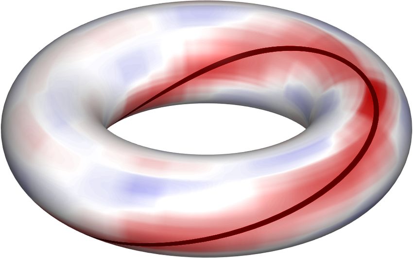
2                                      E. Rodolà et al. / Functional Maps Representation on Product Manifolds

respondence [RCB∗ 17, LRB∗ 16], and cluttered correspondence                i ≥ 1, with real eigenvalues 0 = λ1 ≤ λ2 ≤ . . . and eigenfunctions
[CRM∗ 16] have been proposed as well. Most recently, functional             {φi }i≥1 forming an orthonormal basis of L2 (M) = { f : M →
maps have also been used in conjunction with intrinsic deep learn-          R | h f , f iM < ∞}. Any function f ∈ L2 (M) can thus be rep-
ing methods [LRR∗ 17]. For a comprehensive survey of functional             resented via the Fourier-like series expansion
maps and related techniques, we refer the reader to [OCB∗ 17].
                                                                                                   f (x) =   ∑ h f , φi iM φi (x) .                     (1)
                                                                                                             i≥1
Motivation and contribution. In this paper, we advocate posing
correspondence—and understanding relationships between the ex-              Product manifolds. Given two Riemannian manifolds
isting representations above—in terms of functions on the product           (M, gM ), (N , gN ) of dimension dM and dN with metric tensors
manifold of the source and target. A motivating observation is that         gM , gN , respectively, their product (M × N , gM
                                                                                                                              ⊕ gN ) is
functional maps approximate a distribution representing the corre-                                                                     a
                                                                                                                                           0
                                                                            manifold of dimension dM + dN , where gM ⊕ gN = gM          0 gN is
spondence in the product space as a linear combination of sepa-
rable tensor-product basis functions. This distribution, however, is        the direct sum of the individual metric tensors [GP10], inducing the
supported on a manifold with a dimension lower than that of the             area element da = dx dy. By this definition of product, to each point
product space: For a pair of two dimensional shapes, the distribu-          (x, y) ∈ M × N is attached a tangent space derived by the canon-
tion is supported on a two-dimensional manifold embedded in a               ical isomorphism T(x,y) M × N = Tx M × Ty N (see [Tu11, ex.
four-dimensional space. Consequently, most of the support of the            8.7]). For tangent vectors ξ, η ∈ Tx M and ζ, µ ∈ Ty N , the inner
basis functions is wasted on “empty” regions of the product space.          product h·, ·i of (ξ, ζ), (η, µ) ∈ T(x,y) M × N is given by
Localized bases on the individual domains improve this situation,                    h(ξ, ζ), (η, µ)iT(x,y) M×N = hξ, ηiTx M + hζ, µiTy N .             (2)
but still most of their support is wasted.
  We show how point-to-point maps, functional maps, and soft                  Now let f ∈ F (M), g ∈ F(N ) for some functional space F,
maps all can be understood as (signed) measures on the product and          and denote by f ∧ g the outer product of f and g defined by the
how these representations might be converted to one another. More           mapping
importantly, this viewpoint suggests new techniques to represent                                   f ∧ g : (x, y) 7→ f (x)g(y) .                        (3)
and approximate mappings directly on the product, e.g. by build-
ing a basis from eigenfunctions of the product Laplace–Beltrami             The LB operator ∆M×N obeys the (outer) product rule identity
operator potentially after filtering undesirable matches.                   [Cha84]:

   Our theoretical contributions have practical bearing on the de-                      ∆M×N ( f ∧ g) = (∆M f ) ∧ g + f ∧ (∆N g) .                      (4)
sign of correspondence techniques. After discretizing product man-          Given eigenvectors (φ, ψ) with corresponding eigenvalues (α, β)
ifolds and their Laplace–Beltrami operators, we consider map de-            satisfying ∆M φ = αφ and ∆N ψ = βψ, application of the product
sign and processing problems among two- and three-dimensional               rule yields
shapes. Reasoning about the product manifold leads to compact,
understandable bases for map design that focus resolution in the                        ∆M×N (φ ∧ ψ) = (∆M φ) ∧ ψ + φ ∧ (∆N ψ)
part of the product most relevant to a correspondence task. One of                                           = (α + β)(φ ∧ ψ) .                         (5)
such means is the construction of inseparable bases. To this end,
we propose to compute localized harmonics on the product mani-              This observation leads to a characterization of LB eigenvalues for
fold, and discuss a numerical scheme that keeps the complexity of           product manifolds:
such a computation feasible and, in particular cases, comparable to         Theorem 1 ([BGM71, Proposition A.II.3]) Let ξ be an eigen-
that of the construction of a separable localized basis. We finally         function of the product LB operator ∆M×N with the correspond-
showcase our framework applied to the task of map refinement.               ing eigenvalue γ. Then, there exist some eigenfunctions φ of ∆M
                                                                            and ψ of ∆N with the eigenvalues α and β, respectively, such that
                                                                            ξ = φ ∧ ψ and γ = α + β.
2. Background
                                                                               It is also easy to check that the set of eigenfunctions {φi ∧ ψ j }i, j
Manifolds. We model shapes as Riemannian d-manifolds                        is orthogonal, since:
(M, gM ) (possibly with boundary ∂M) equipped with area                      Z                                         Z
elements dx induced by the standard metric gM ; we do not restrict                    (φi ∧ ψ j )(φk ∧ ψ` ) da =             φi (x)ψ j (y)φk (x)ψ` (y) da
our focus to surfaces but rather allow M and N to have different              M×N                                      M×N
                                                                                                   Z               Z
intrinsic dimensions. We denote by Tx M the tangent plane at                                   =       φi φk dx   ψ j ψ` dy                             (6)
x ∈ M, modeling the manifold locally as a Euclidean space. Given                                   M

                                                                                                                N
two scalar functions f , g : M → R belonging to an appropriate                                                  1 (i = k) and ( j = `);
                                                                                                = δik δ j` =                                            (7)
functional space F(M),
                    R
                             we use the standard manifold inner                                                 0 otherwise,
product h f , giM = M f (x)g(x) dx.
                                                                            where δi j is the Kronecker delta.
   In analogy to the Laplace operator in flat spaces, the posi-
tive semidefinite Laplace–Beltrami (LB) operator ∆M equips us               Soft maps. A soft map µ̃ : M → Prob(N ) is a function assign-
with the tools to extend Fourier analysis to manifolds. The man-            ing a probability measure over N to each point in M [SNB∗ 12].
ifold Laplacian admits an eigen-decomposition ∆M φi = λi φi for             Soft maps can be equivalently represented by their densities, i.e.,

                                                                                                              submitted to COMPUTER GRAPHICS Forum (1/2019).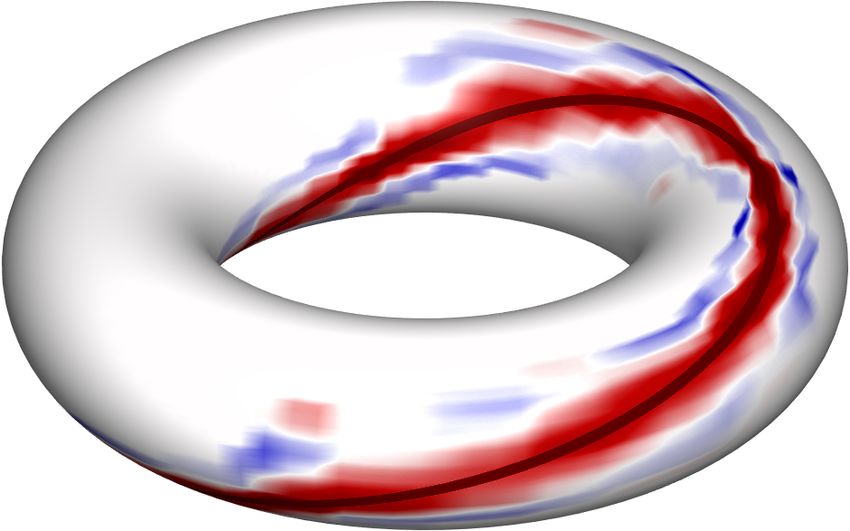
E. Rodolà et al. / Functional Maps Representation on Product Manifolds 3
j
j
1 k in applications requiring additional efficiency, lumped mass matri-
h βi j αi j k αi j
ces diag(ŝii ) can be used by setting ŝii = ∑ j si j .
i i The product of two boundary-free 1D manifolds M, N is a 2D
ei j e jk
manifold (a surface) M × N with torus topology. For the dis-
i j k
cretization of the Laplacian on M × N , we appeal to the following:
(a) (b)
Figure 1: Discretization of the Laplace-Beltrami operator on a cy- Theorem 2 (Discrete product Laplacian) Let M, N be 1D man-
cle graph (a) and on a triangle mesh (b) for interior (green) and ifolds with no boundary, discretized as 2-regular cycle graphs, and
boundary edges (red). We also show the hat basis function in (a). let SM , WM and SN , WN be the mass and stiffness matrices for
∆M and ∆N respectively, obtained via FEM with respect to piece-
wise linear (hat) basis functions. Then,
nonnegative scalar functions µ : M × N → [0,R 1] defined on the SM×N = SM ⊗ SN (12)
product manifold M × N satisfying µ̃(x)(B) = B⊆N µ(x, y) dy for WM×N = WM ⊗ SN + SM ⊗ WN (13)
all x ∈ M and all measurable subsets B ⊆ N .
are the mass and stiffness matrices for the product manifold Lapla-
As a particular case, a bijection π̃ : M → N induces a soft map cian ∆M×N with respect to piecewise bilinear basis functions, de-
µ̃ by requiring, for all x ∈ M, that µ̃(x)(B) = 1 if and only if π̃(x) ∈ fined on a quad meshing of the toric surface M × N . Here, ⊗ de-
B ⊆ N , i.e., the image µ̃(x) is a unit Dirac mass δπ̃(x) centered at notes the Kronecker product.
π̃(x).
Proof See Appendix A.
Functional maps. A functional map T associated to a map π̃ : Corollary 1 The LB operator ∆M×N is discretized as:
M → N is a linear mapping T : F(N ) → F(M) defined as
[OBCS∗ 12]: LM×N = LM ⊗ IN + IM ⊗ LN , (14)
T (g) = g ◦ π̃ . (8) where IM , IN are nM × nM and nN × nN identity matrices.
Proof See Appendix A.
Note how this construction allows to move from identifying a
map between manifolds to identifying a linear operator between The discretization of ∆M×N does not require the explicit con-
Hilbert spaces. The functional map T admits a matrix representa- struction of a quad mesh embedded in R3 ; the toric shapes shown
tion wrt orthogonal bases {φi }i≥1 , {ψ j } j≥1 on F(M) and F(N ) in these pages only serve visualization purposes. Further, the dis-
respectively, with coefficients C = (ci j ) determined as follows: cretization (14) is consistent with the spectral decomposition iden-
tities (5); see [Fie73] and [HIK11, Proposition 33.6] for additional
T (g) = ∑ hψ j , giN hφi , T (ψ j )iM φi . (9)
i j≥1 ´¹¹ ¹ ¹ ¹ ¹ ¹ ¹ ¹ ¹ ¹ ¹ ¹ ¹ ¹ ¹ ¸ ¹ ¹ ¹ ¹ ¹ ¹ ¹ ¹ ¹ ¹ ¹ ¹ ¹ ¹ ¹ ¶ discussion.
ci j
2D shapes (surfaces). We model 2D surfaces as manifold triangle
3. Discretization meshes (V, E, F) with n vertices V connected by edges E = Ei ∪ Eb
(where Ei and Eb are interior and boundary edges, respectively) and
We show how to discretize the main quantities involved in our triangle faces F. In analogy to the 1D case, the discretization of
framework on 1D and 2D manifolds, as well as their products. the LB operator is obtained using FEM with piecewise linear basis
functions on triangle elements [Duf59], taking the form of an n × n
1D shapes (curves). We model 1D manifolds as closed contours sparse matrix L = S−1 W, where
with circular topology (no boundary), discretized as 2-regular cycle
graphs G = (N , E) with n ≥ 3 nodes N and as many edges E. The
(cot αi j + cot βi j )/2 i j ∈ Ei
LB operator ∆ is discretized using standard FEM with linear hat (cot α )/2
ij i j ∈ Eb
wi j = (15)
functions; in the hat basis, scalar functions on G are approximated
− ∑ k6=i w ik i =j
piecewise-linearly on the edges. The Laplacian takes the form of a
0 otherwise, and
n × n sparse matrix L = S−1 W, where:
1 (A(Thi j ) + A(Ti jk ))/12 i j ∈ Ei
− kei j k
ei j ∈ E
A(T )/12 i j ∈ Eb
wi j = − ∑i6=k wik i = j (10) si j = 1 i jk (16)
∑
6 k∈N (i) A(Tk ) i= j
0 otherwise
0 otherwise.
1
6 kei j k
ei j ∈ E
Here, A(T ) denotes the area of triangle T and N (i) is the set of the
1
si j = 3 ∑k∈N (i) keik k i = j (11)
neighbors of vertex i; see Figure 1 for notation.
0 otherwise
Given two 2D manifolds M and N , their product is a 4D mani-
and the notation is according to Figure 1, with N (i) being the set of fold M × N . The LB operator on M × N is discretized similarly
the neighbors of node i. In our tests we use non-lumped masses si j ; to the lower-dimensional case:
submitted to COMPUTER GRAPHICS Forum (1/2019).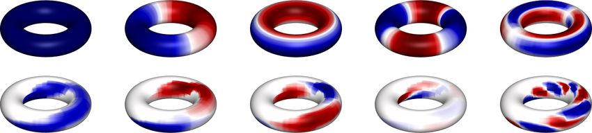
4 E. Rodolà et al. / Functional Maps Representation on Product Manifolds
1
× = × =
0
(a) (b)
Figure 2: The Cartesian product of two edge elements is a quad
(a), while taking the product of two triangles yields a 4D geometric (a) (b) (c)
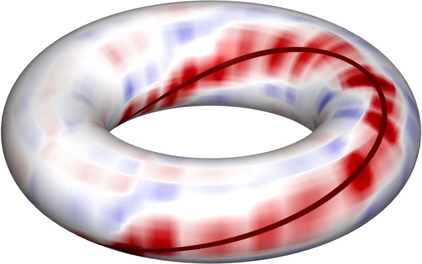
structure called a 3-3 (or triangular) duoprism [Cox48] visualized Figure 3: The ground truth map (here the identity) between two
with a Schlegel diagram [Sch83] (b). Note that all these objects are shapes approximated according to (a) the standard functional map
polytopes (i.e. they have faces), not simple graphs. representation, (b) the (separable) LB eigenfunctions of the prod-
uct manifold, ordered according to the product eigenvalues, and (c)
the (inseparable) localized harmonics on the product manifold. All
Corollary 2 Let M, N be surfaces discretized as triangle meshes, three cases use the same amount of coefficients. The black curve in
and let SM , WM and SN , WN be the mass and stiffness matri- each matrix represents the maximum value for each row. In this ex-
ces for ∆M and ∆N . Then, equations (12)-(14) provide a valid dis- ample the product manifold is a flat torus, represented in the para-
cretization of the LB operator ∆M×N . This discretization is equiv- metric domain in (a), (b), (c).
alent to the application of FEM on a 3-3 duoprism tessellation of
the 4D product manifold M × N using multilinear basis functions.
Proof See Appendix A. let ci j = hφi , Tµ (ψ j )iM be the matrix coefficients of Tµ in the or-
thogonal bases {φi }i≥1 , {ψ j } j≥1 , and let pi j = hφi ∧ ψ j , µiM×N
We emphasize that, as a consequence of the Corollary, the com-
be the expansion coefficients of µ in the product basis {φi ∧ ψ j }i, j ,
putation of the product Laplacian ∆M×N does not require con-
such that µ = ∑i j (φi ∧ ψ j )pi j . Then, ci j = pi j for all i, j.
structing a high-dimensional embedding for M × N , thus avoid-
ing cumbersome manipulation of duoprismic product elements (see Proof The functional map matrix coefficients are computed as:
Figure 2 for an illustration of these elements). Z
ci j = hφi , Tµ (ψ j )iM = φi (x)Tµ (ψ j )(x) dx (18)
Finally, scalar functions on a manifold M are represented by n-
ZM
dimensional vectors f = ( f (x1 ), . . . , f (xn ))> , where x1 , . . . , xn de-
Z
= φi (x) ψ j (y)µ(x, y) dy dx (19)
note graph nodes and mesh vertices in the 1D and 2D case respec-
ZM N
tively. Inner products h f , giM are discretized as f> Sg, where S is
= φi (x)ψ j (y)µ(x, y) da , (20)
the mass matrix. On product manifolds, scalar functions are rep- M×N
resented as nM × nN matrices F, usually deriving from an outer
while the expansion coefficients of µ are given by
product f ∧ g discretized as fg> ; inner products are computed as
vec(F)> S vec(G) (vec(F) stacks the columns of F into a vector).
Z
pi j = hφi ∧ ψ j , µiM×N = φi (x)ψ j (y)µ(x, y) da . (21)
M×N
4. Map representation on the product manifold Comparing equations (20) and (21), we see that ci j = pi j for any
choice of i, j ≥ 1.
Soft functional maps. It will be instrumental for our purposes to
introduce a “soft” generalization of functional maps. For soft maps Note that Theorem 3 applies to any choice of orthogonal bases
µ̃ : M → Prob(N ) with associated density µ ∈ L1 (M × N ), we {φi }i≥1 ∈ F (M), {ψ j } j≥1 ∈ F (N ).
define a soft functional map Tµ : F(N ) → F (M) as the expectation Spectral representation. Consider the order-k, band-limited ap-
Z
proximation of µ:
Tµ (g)(x) = g(y)µ(x, y) dy . (17)
N k
µ≈ ∑ ξ` p` , (22)
It is easy to check that Tµ is linear in g, hence admitting a ma- `=1
trix representation with coefficients defined as in (9); in particular,
where each ξ` is an eigenfunction of ∆M×N which uniquely iden-
in the standard basis one obtains a stochastic matrix with each row
tifies, via (5), a pair of eigenfunctions φi , ψ j on M and N respec-
summing to 1. If the density µ encodes a non-soft map (i.e., when-
tively. According to Theorem 3, the expansion coefficients p` are
ever µ(x, ·) is concentrated at one point), theRdefinition (17) boils
exactly those appearing in the functional map matrix C, when this
down to the original definition (8), T (g)(x) = N g(y) δπ̃(x) (y) dy =
is expressed in the Laplacian eigenbases of M and N as originally
(g ◦ π̃)(x), where the last equivalence stems from the sampling
proposed by Ovsjanikov et al. [OBCS∗ 12]. There is, however, a
property of Dirac deltas.
crucial difference in the way the two sets of coefficients are stored.
We begin our discussion by deriving a connection between We come to the following observation:
functional map matrices and expanding soft map measures in the
Truncation. The product eigenfunctions ξ` appearing in the sum-
Laplace–Beltrami basis:
mation (22) are associated to the product eigenvalues αi + β j ,
Theorem 3 (Equivalence) Let Tµ : F(N ) → F(M) be a soft func- which are ordered non-decreasingly. In contrast, in [OBCS∗ 12]
tional map (17) with underlying density µ ∈ L1 (M × N ). Further, it was proposed to truncate the two summations in (9) to i =
submitted to COMPUTER GRAPHICS Forum (1/2019).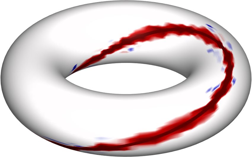
E. Rodolà et al. / Functional Maps Representation on Product Manifolds                                           5

                  Laplacian spectrum          Functional map coefficients                    5. Spectral map processing
                                                                                  1
                                              1
              8
                           C                                                                 In this paper, we consider curves and surfaces as our shapes. De-
                                                                                             spite their different intrinsic dimensions, our framework applies to
 Eigenvalue

              6
                                                                                             both without specific adjustment.
                                                                                  0.5
              4
                                                                                             Localized spectral encoding. Theorem 3 establishes the equiva-
              2                                                                              lence between the soft functional map Tµ representation coefficients
                                             10
                                                                                             ci j in the bases {φi }i≥1 ⊆ F (M) and {ψ j } j≥1 ⊆ F(N ) and the
              0                                                                   0
                  0   50   100   150   200        1                 10                       coefficients p` of the underlying density µ Fourier series (22) in the
                                                                                             eigenbasis {ξ` }`≥1 ⊆ F(M × N ) of the product manifold Lapla-
Figure 4: Left: The k = 100 frequencies involved in the construc-                            cian ∆M×N . This equivalence directly stems from ξ` ’s having the
tion of a 10 × 10 functional map matrix C correspond to an irreg-                            separable form φi ∧ ψ j , by virtue of Theorem 1. It may be advanta-
ular sampling of the Laplacian spectrum of the product manifold.                             geous, however, to consider different orthonormal bases on M×N
Right: In turn, only some of the coefficients ci j of matrix C ap-                           that are not necessarily separable. In particular, we observe that µ
pear among the first k expansion coefficients pi j of the map in the                         tends to be localized on the product manifold M × N (see Fig-
product eigenbasis. Here C is framed in black, while the blue dots                           ure 3), and thus the standard outer product basis is extremely waste-
identify the first k coefficients pi j .                                                     ful as it is supported on the entire M × N .
                                                                                                A better alternative is the use of localized manifold harmonics
                                                                                             [CSBK17,MRCB18]. Assume that we are given a rough indication
                                                                                             of the support of µ (for example, coming from a shape matching
1, . . . , kM and j = 1, . . . , kN , where indices i and j follow the non-                  algorithm) in the form of a step potential function
decreasing order of the eigenvalue sequences αi and β j separately.
                                                                                                                              ν µ(x, y) ≈ 0;
                                                                                                                V (x, y) =                                 (24)
    We see that, due to the different ordering, the eigenfunctions                                                            0 otherwise.
φi , ψ j involved in the approximation (22) of µ are not necessarily all
                                                                                             where ν ≥ 1. Then, the variational problem
those involved in the construction of C (9), assuming k = kM kN .
In the former case we operate with a reduced basis directly on                                                k Z
M × N , while in the latter case we consider two reduced bases                                       min     ∑               k∇M×N ξ` k2gM ⊕gN +V ξ2` da (25)
                                                                                                    ξ1 ,...,ξk `=1 M×N
on M and N independently. This has direct implications on the
quality of the approximated maps, as illustrated in Figure 3.                                           s.t. hξ` , ξ`0 iM×N = δ`,`0

Relation to finite sections. The functional map representation was                           produces a set of orthonormal functions denoted by ξˆ 1 , . . . , ξˆ k that,
originally introduced in [OBCS∗ 12] as a convenient language for                             for a sufficiently large value of ν, are also localized in the support
solving map inference problems of the type [OCB∗ 17]:                                        of V . Note that this new basis {ξˆ ` }k`=1 is no longer separable, i.e.,
                                                                                             the functions ξˆ are not in general expressible as outer products of
                                             CA = B ,                            (23)
                                                                                             functions defined on the originating domains. See Figures 5 and 6
where matrices B = (hφi , f j iM ), A = (hψi , g j iN ) contain Fourier                      for an illustration, and Figures 7 and 8 for practical examples.
coefficients of a given set of corresponding “probe” functions                                  The basis {ξˆ ` }k`=1 turns out to be the eigenbasis of the Hamilto-
 f j , g j , j = 1, . . . , q on M and N respectively (typically, descrip-                   nian operator [CSBK17] H = ∆M×N + V and can be computed
tors are used). In the problem above, one is asked to estimate the                           by the eigendecomposition of the product Laplacian matrix with
functional map C.                                                                            the addition of diagonal potential. The size of such problem can be
   By truncating the matrix C to the left upper kM × kN subma-                               huge (if the shapes are discretized with n ∼ 103 points, the product
trix (as in [OBCS∗ 12]), one obtains a finite-dimensional approx-                            Laplacian matrix has size n2 × n2 = 106 × 106 ; see Theorem 2),
imation of the infinite linear system (23). This procedure, known                            and despite its extreme sparsity, computationally expensive.
as the finite section method [GRS10], does not always guarantee                                As an alternative, we consider a patch P ⊂ M × N of the prod-
convergence, and a series of remedies using rectangular sections                             uct manifold with boundary ∂P corresponding to µ(x, y) > 0, and
(kM 6= kN ) have been proposed in the literature (see [GO17] for a                           define the eigenproblem
discussion pertaining to functional maps).
                                                                                                           ∆P ξ¯ ` (x, y) = γ` ξ¯ ` (x, y)   (x, y) ∈ int(P)
   Recall that, according to Theorem 3, the matrix elements ci j cor-                                                                                               (26)
                                                                                                           ξ¯ ` (x, y) = 0                   (x, y) ∈ ∂P
respond to the expansion coefficients pi j appearing in (22). Thus,
due to the different ordering of the pi j ’s, the approximation carried                      of the product patch Laplacian ∆P with homogeneous Dirichlet
out in (22) can be regarded as an “irregular” finite section (see Fig-                       boundary conditions. In practice, this is implemented by construct-
ure 4, right); in contrast with purely algebraic approaches consider-                        ing the stiffness and mass matrices Wint(P) , Sint(P) by selecting the
ing general systems of linear equations such as (23), our approach                           rows and columns of WM×N , SM×N that correspond to the ver-
carries now a geometric meaning in that the shape of the section is                          tices in int(P). A generalized eigenproblem using Wint(P) , Sint(P)
determined by the geometry of the product manifold.                                          is solved, yielding eigenfunctions ξ¯ int(P) defined on int(P); the fi-

submitted to COMPUTER GRAPHICS Forum (1/2019).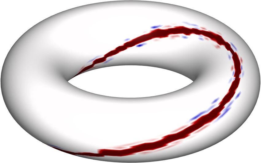
6                                       E. Rodolà et al. / Functional Maps Representation on Product Manifolds

         Eigenfunction 1                    3                             5                          10                                20
Figure 5: Basis functions on the product manifold (here visualized as a torus embedded in R3 ) of two 1D shapes. We plot a few standard LB
eigenfunctions (top row) and localized manifold harmonics (bottom row). Here and in the following, we use the present color scheme (blue
denotes small values, red large values, white is zero).

                                                                              framework, we propose a simple procedure for map refinement:
                                                                              Given some initial, possibly sparse and noisy correspondence, the
                                                                              task is to produce a dense, denoised map.
                                                                                 We follow an iterative approach. In each iteration k, the map
                                                                              is represented as a density µ(k) : M × N → [0, 1]. This density is
                                                                              interpreted as a heat distribution throughout the iterations.
                                                                                  At the k-th iteration, a diffusion process is initialized with
                                                                                (k)
                                                                              ut=0 := µ(k) and solved for a given diffusion time T (k) on a patch
                                                                              P (k) . The initial patch can be given or be the entire product mani-
                                                                              fold. The diffusion process has the effect of spreading correct corre-
                                                                              spondence information and therefore suppress mismatches, result-
                                                                              ing in an effective map denoising approach akin to diffusion-based
Figure 6: Projecting the basis functions on the product manifold              smoothing from image processing [Wit83, PM90]. The final heat
of horse and elephant back onto the factor shapes (here only the                              (k)
                                                                              distribution uT is thresholded to define a patch P (k) ⊂ M × N
horse projection is visualized). Top row: Projection of three prod-
                                                                              where the correct correspondence is likely to be contained, with
uct LB eigenfunctions, which correspond exactly to three standard
                                                                              likelihood expressed in terms of the diffused density. We then re-
LB eigenfunctions on the horse shape. Bottom row: Projection of                                                                     (k)
three localized harmonics; these projections do not correspond to             cover a bijective (non-soft) density µ(k+1) from uT by solving a
any LB eigenfunction on the horse. Still, note how they capture the           linear assignment problem [Ber98] restricted to region P (k) , and
geometric features of the underlying shape.                                   use it to initialize the next iteration.
                                                                                 These blur-and-sharpen steps are iterated until convergence
                                                                              while decreasing T (k) , resulting in a sequence P (0) ⊇ · · · ⊇ P (k) ⊇
nal eigenfunctions ξ¯ on the entire patch P are obtained by setting           P (k+1) . In practice, we decrease T (k) logarithmically across itera-
¯                                  ¯
     = ξint(P) for x ∈ int(P) and ξ(x)  = 0 for x ∈ ∂P.
ξ(x)                                                                          tions. At k = 0, the density u(0) is the given input, e.g., a mixture
   If the patch is selected in such a way that its size scales as O(n)        of Dirac deltas or a soft map.
rather than O(n2 ) in the size of the shapes (in practice, this can             The diffusion step in each iteration is realized via the spectral
be achieved by taking a fixed-size band around the initial corre-             decomposition of the product patch Laplacian ∆P with Dirichlet
spondence), the computation of the localized basis {ξ¯ ` }k`=1 has the        boundary conditions on P = P (k) (26); for p, q ∈ M × N :
same complexity as eigendecomposition of the individual Lapla-                                             Z
cians ∆M , ∆N . An example application of this construction is de-                              uT (p) =          hT (p, q)u0 (q)dq                    (27)
scribed next.                                                                                              M×N

   Despite the computational gains of working with patches P ⊂                                hT (p, q) =  ∑  e−T γ` ξ¯ ` (p)ξ¯ ` (q) ,                (28)
                                                                                                          `≥0
M × N , computing the eigen-decomposition of the full Hamilto-
nian ∆M×N + V may still be useful in certain settings. Note, in               where hT is the heat kernel at time T on the product manifold
particular, that one may define a soft potential V (x, y) = 1 − µ(x, y)       M × N . Throughout the iterations we keep the number of eigen-
[MRCB18] directly reflecting the reliability of the underlying map            functions for the approximation (28) constant.
in terms of its density. Further, it is also possible to define a patch
                                                                                 The refinement process described above simultaneously im-
Hamiltonian ∆P +V |P with soft potential if desired.
                                                                              proves the correspondence and reduces the support of the den-
Example: Map refinement. As an illustrative application of our                sity around the most likely bijective map. This is similar in spirit

                                                                                                               submitted to COMPUTER GRAPHICS Forum (1/2019).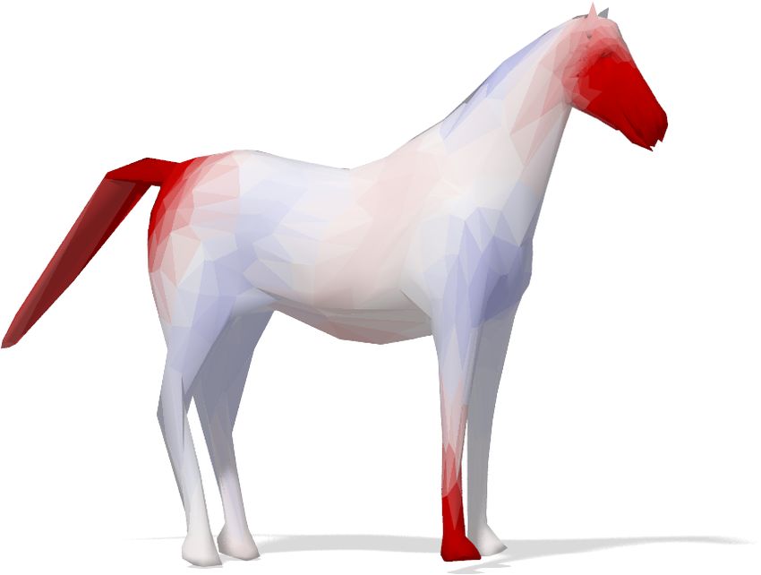
E. Rodolà et al. / Functional Maps Representation on Product Manifolds                                   7

                       100
  % Correspondences

                        80
                                                          1%
                        60
                                                          5%
                        40                                25%
                                                          90%                  Source
                        20
                                                          FM
                         0
                             0    0.02     0.04   0.06    0.08    0.1
                                         Geodesic error                                             FM                90%               25%             5%              1%
Figure 7: Product space approximation of the correspondence between one-dimensional shapes with k = 100 basis functions. Bases con-
structed on bands of different size (1%, 5%, 25% and 90% of the total product manifold area) around the true correspondence are shown.
Separable basis (FM) is shown as a reference. Left: accuracy of the correspondence increases as the product space basis becomes more
localized. Right (top row): image of a delta function by the functional maps. Right (bottom row): True correspondence (curve) and its
approximation in inseparable product space bases with a varying degree of localization. The product manifold is depicted as a torus.

                       100
                                                                                 source
   % Correspondences

                        80

                        60

                        40                                15%
                                                          10%
                        20
                                                          FM
                         0
                             0    0.02     0.04   0.06   0.08    0.1
                                         Geodesic error

                                                                                                                                                                         0.1

                                                                                                                                                                         0
                             FM                            15%                            10%
Figure 8: Map approximation between surfaces with k = 500 ba-
sis functions on bands of different size (10% and 15% of the to-
tal 4D product manifold area) around the true correspondence. We
also show images on the horse of delta functions supported at three
points (red, green, blue) on the elephant. Here, the functional map
(FM) was calculated using 30 × 30 = 900 basis functions.

to the kernel matching approaches of [VLR∗ 17, VLB∗ 17], how-                                                  Figure 9: Example of map refinement. We show the input sparse
ever, with the additional step of ‘carving out’ the relevant portion                                           correspondence above and the recovered dense map below. The
P ⊂ M × N throughout the iterations.                                                                           heatmap on the bottom right encodes geodesic error of the recov-
                                                                                                               ered correspondence.
  Illustrative results are reported qualitatively in Figure 9 and
quantitatively in Figure 10.

6. Discussion and conclusions                                                                                  ‘wasted’ on portions of the product manifold that carry no infor-
                                                                                                               mation on the map to be encoded. Our theoretical and applied con-
We introduced a novel perspective on map representation and pro-
                                                                                                               tributions suggest a new perspective on properties of the correspon-
cessing, where pointwise, functional, and soft maps can be under-
                                                                                                               dence manifold as well as new ways to pose algorithmic design for
stood as densities on the product of the input shapes. We showed
                                                                                                               map inference and processing.
how to discretize the Laplace-Beltrami operator on the product
manifold and proposed the adoption of (inseparable) localized har-                                             Limitations. Perhaps the main limitation of our framework lies in
monics for compactly encoding correspondences while ensuring                                                   the scalability of our current numerical scheme. While we showed
minimal energy dispersion, i.e., the resulting harmonics are not                                               that one can reduce the computational complexity to O(n) by ap-

submitted to COMPUTER GRAPHICS Forum (1/2019).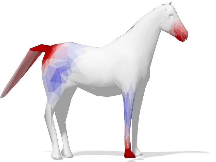
8 E. Rodolà et al. / Functional Maps Representation on Product Manifolds
100 100 proposed discretization of the (product) Laplace-Beltrami operator,
as well as its spectral decomposition, can be directly employed in
80 80 such pipelines, enabling new forms of structured prediction in a
% Correspondences
range of challenging problems in vision and graphics.
60 60
(0.1, 0.01)
40 (1, 0.01) 40 Acknowledgments
(10, 0.1)
We gratefully acknowledge Mathieu Andreux, Matthias Vestner, Michael
(100, 1)
20 20 Moeller, Maks Ovsjanikov, and Paolo Rodolà for fruitful discussions. ER
(1000, 0.01)
(1000, 10)
is supported by the ERC grant no. 802554 (SPECGEO). AB is supported
0 0
by the ERC grant no. 335491 (RAPID). MB is supported in part by the
0 0.02 0.04 0.06 0.08 0.1 0 0.02 0.04 0.06 0.08 0.1 ERC grant no. 724228 (LEMAN), Royal Society Wolfson Research Merit
Geodesic error Geodesic error Award, Google Research Faculty Awards, Amazon AWS Machine Learn-
ing Research Award, and the Rudolf Diesel fellowship at the Institute for
Figure 10: Sensitivity of map refinement to heat diffusion times and
Advanced Studies, TU Munich. JS acknowledges the generous support of
noisy input. The legend reports diffusion time ranges (tmax ,tmin );
Army Research Office grant W911NF-12-R-0011 (“Smooth Modeling of
within each range, time is decreased logarithmically over itera-
Flows on Graphs”), of National Science Foundation grant IIS-1838071
tions. Left: The input is a sparse correspondence of 10% of correct
(“BIGDATA:F:Statistical and Computational Optimal Transport for Geo-
matches. We see that high diffusion times are detrimental due to
metric Data Analysis”), from the MIT Research Support Committee, from
the excessive spread of correspondence information. Right: The in-
an Amazon Research Award, from the MIT–IBM Watson AI Laboratory,
put sparse correspondence is further corrupted with 30% random
and from the Skoltech–MIT Next Generation Program.
mismatches.
Appendix A: Proofs
propriately selecting a localization region, in practical applications
involving very noisy maps where the localization region tends to be We provide proofs for the main propositions of the paper.
spread out across the entire product manifold, the advantage might Proof of Theorem 2. Following standard FEM, we discretize the
be less evident. For this reason, considering as a possible exten- Poisson equation ∆M×N f = g via the weak formulation
sion higher-dimensional products to encode cycle-consistent maps
in shape collections may soon become prohibitive. With the cur- h∆M×N f , H j i = hg, H j i , (29)
rent approach we trade off scalability for accuracy: Maps are en-
coded much more precisely in the localized basis, but this requires where functions are expressed in the hat basis {H j : M × N →
the explicit computation of inseparable basis functions that do not R}, and are thus approximated piecewise-linearly via the expansion
admit an efficient representation in terms of outer products. As a f (x) ≈ ∑ni=1 f (vi )hi (x). The left-hand side of (29) can be written as
possible remedy, an efficient solution to the eigenproblem might be h∆ f , H j i = −h∇ f , ∇H j i = − ∑ f (vi ) h∇Hi , ∇H j i , (30)
sought via approximation methods similar to [NBH18]. A second i ´¹¹ ¹ ¹ ¹ ¹ ¹ ¹ ¹ ¹ ¹ ¹ ¹ ¸¹¹ ¹ ¹ ¹ ¹ ¹ ¹ ¹ ¹ ¹ ¹ ¹ 
limitation is in our map refinement scheme, which has limited re- wi j
silience to particularly noisy input. We presented our algorithm as where wi j are elements of the stiffness matrix W. The right-hand
an illustrative tool for map denoising, but more effective schemes side of (29) can be written as
operating on the product manifold are likely possible.
hg, H j i = h∑ g(vi )Hi (x), H j i = ∑ g(vi ) hHi , H j i , (31)
´¹¹ ¹ ¹ ¹ ¹ ¸¹¹ ¹ ¹ ¹ ¹
Future work. From an investigative standpoint, it might be worth i i
considering a notion of optimal transport between maps as a means si j
of exploring the space of maps between given shapes, a natural
choice given our modeling of maps as measures on a manifold. where si j are elements of the mass matrix S.
Related constructions could extend distortion measures like the The Cartesian product of the two graphs discretizing M and
Dirichlet energy [Bre03, SGB13, Lav17] to the functional regime. N has grid topology, as illustrated in Figure 11, and the result-
Another particularly interesting direction will be to consider gen- ing bilinear hat basis functions are expressed via the outer product
eral graphs (as opposed to manifolds) and their products in the con- He = h j ∧ hq . We can then compute the mass values (refer to the
text of network analysis, machine learning, and applications. While Figure for the color notation):
many of our results may be directly translated to graphs, the lack of see = hHe , He i = hh j ∧ hq , h j ∧ hq i
differentiable structure poses new theoretical challenges and at the Z
same time provides a richer spectrum of possibilities; for example, = h j (x)hq (y)h j (x)hq (y)dxdy
several different notions of product exist between graphs [HIK11]. Qabde ∪Qbce f ∪Qdegh ∪Qe f hi
Z Z
Finally, a promising direction is the introduction of product = h j (x)h j (x)dx hq (y)hq (y)dy
Ei jk E pqr
spaces within geometric deep learning [BBL∗ 17] pipelines, where
the data is in the form of signals defined on top of a manifold. Our = s j j sqq (32)
submitted to COMPUTER GRAPHICS Forum (1/2019).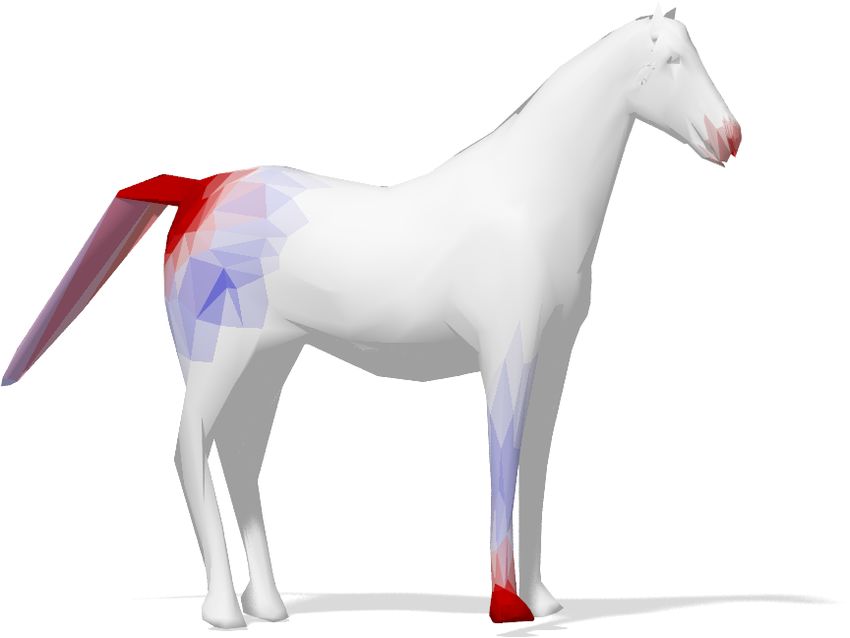
E. Rodolà et al. / Functional Maps Representation on Product Manifolds 9
i j k
.. · · · ···
sae = hHa , He i = hhi ∧ hr , h j ∧ hq i . a b c
Z r
= hi (x)hr (y)h j (x)hq (y)dxdy Hf
Qabde He
Z Z
q d e f
= hi (x)h j (x)dx hr (y)hq (y)dy
Ei j Eqr
e f
= si j sqr (33) i
p. h
.. g h i
sde = hHd , He i = hhi ∧ hq , h j ∧ hq i Figure 11: Left: The product of two closed contours discretized as
Z
= hi (x)hq (y)h j (x)hq (y)dxdy cycle graphs (in blue and red) is a quad mesh with toric topology
Qabde ∪Qdegh (in grey). Uniform edge lengths are used for illustration purposes.
Right: Two overlapping bilinear hats He and H f . On the quad el-
Z Z
= hi (x)h j (x)dx hq (y)hq (y)dy
Ei j E pqr ement Qe f hi (marked in red) there is non-zero overlap, hence it
contributes to the computation of mass and stiffness values.
= si j sqq (34)
Similarly, the stiffness integrals read:
Proof of Corollary 2. Since triangular (3-3) duoprisms are, by def-
wee = h∇He , ∇He i = h∇h j ∧ hq , ∇h j ∧ hq i
inition, the Cartesian product of two triangles, we can define a mul-
= h∇h j hq , ∇h j hq i + 2hh j ∇hq , ∇h j hq i + hh j ∇hq , h j ∇hq i tilinear basis function on the product complex as the outer product
Z
of two standard hats defined on triangle meshes. We are now in
= h∇h j (x)hq (y), ∇h j (x)hq (y)idxdy + · · ·
Qabde ∪Qbce f ∪Qdegh ∪Qe f hi the same setting as the lower dimensional case, and in particular
Z Equations (32)-(37) remain valid.
= hq (y)hq (y)h∇h j (x), ∇h j (x)idxdy + · · ·
Qabde ∪Qbce f ∪Qdegh ∪Qe f hi
Z Z
References
= h∇h j (x), ∇h j (x)idx hq (y)hq (y)dy + · · · + · · ·
Ei jk E pqr [ADK16] A FLALO Y., D UBROVINA A., K IMMEL R.: Spectral general-
= w j j sqq + s j j wqq (35) ized multi-dimensional scaling. IJCV 118, 3 (2016), 380–392. 1
[BBL∗ 17] B RONSTEIN M. M., B RUNA J., L E C UN Y., S ZLAM A.,
wae = h∇Ha , ∇He i = h∇hi ∧ hr , ∇h j ∧ hq i VANDERGHEYNST P.: Geometric deep learning: Going beyond eu-
clidean data. IEEE Signal Processing Magazine 34, 4 (July 2017), 18–
= h∇hi hr , ∇h j hq i + hhi ∇hr , h j ∇hq i 42. 8
= wi j sqr + si j wqr (36) [Ber98] B ERTSEKAS D. P.: Network Optimization: Continuous and Dis-
crete Models. Athena Scientific, 1998. 6
wde = h∇Hd , ∇He i = h∇hi ∧ hq , ∇h j ∧ hq i [BGM71] B ERGER M., G AUDUCHON P., M AZET E.: Le spectre d’une
variété Riemannienne. Lecture notes in mathematics. Springer-Verlag,
= h∇hi hq , ∇h j hq i + hhi ∇hq , h j ∇hq i 1971. 2
= wi j sqq + si j wqq (37) [Bre03] B RENIER Y.: Extended monge-kantorovich theory. In Optimal
transportation and applications. Springer, 2003, pp. 91–121. 8
where we applied the outer product rule for the gradient operator,
and used the fact that h∇ f , ∇gi = 0 for any pair of functions on the [Cha84] C HAVEL I.: Eigenvalues in Riemannian geometry, second ed.
Academic Press, 1984. 2
two cycle graphs. Note the integrals sae and wae are non-zero even
if nodes a and e are not connected in the product graph. [Cox48] C OXETER H. S. M.: Regular Polytopes. Dover Publications,
1948. 4
In matrix notation, formulas (32)-(37) can be succinctly written [CRA∗ 17] C OSMO L., RODOLÀ E., A LBARELLI A., M ÉMOLI F., C RE -
as: MERS D.: Consistent partial matching of shape collections via sparse
modeling. Computer Graphics Forum 36, 1 (2017), 209–221. 1
S = S⊗S
[CRM∗ 16] C OSMO L., RODOLÀ E., M ASCI J., T ORSELLO A., B RON -
W = W⊗S+S⊗W, STEIN M. M.: Matching deformable objects in clutter. In Proceedings
- 2016 4th International Conference on 3D Vision, 3DV 2016 (Stanford,
completing the proof. 2016), IEEE, pp. 1–10. 2
Proof of Corollary 1. The proof is straightforward and follows [CSBK17] C HOUKROUN Y., S HTERN A., B RONSTEIN A., K IMMEL R.:
from substituting the expressions (12), (13) into the general formula Hamiltonian operator for spectral shape analysis. arXiv:1611.01990v2
L = S−1 W: (2017). 1, 5
[Duf59] D UFFIN R. J.: Distributed and lumped networks. Journal of
LM×N = S−1
M×N WM×N Mathematics and Mechanics 8, 5 (1959), 793–826. 3
= (SM ⊗ SN )−1 (WM ⊗ SN + SM ⊗ WN ) [EBC17] E ZUZ D., B EN -C HEN M.: Deblurring and denoising of maps
between shapes. Computer Graphics Forum 36, 5 (2017), 165–174. 1
= (S−1 −1 −1 −1
M ⊗ SN )(WM ⊗ SN ) + (SM ⊗ SN )(SM ⊗ WN ) [ERGB16] E YNARD D., RODOLÀ E., G LASHOFF K., B RONSTEIN
= (S−1 −1 −1 −1
M WM ) ⊗ (SN SN ) + (SM SM ) ⊗ (SN WN )
M. M.: Coupled functional maps. In Proceedings - 2016 4th Inter-
national Conference on 3D Vision, 3DV 2016 (Stanford, 2016), IEEE,
= L M ⊗ IN + IM ⊗ L N . pp. 399–407. 1
submitted to COMPUTER GRAPHICS Forum (1/2019).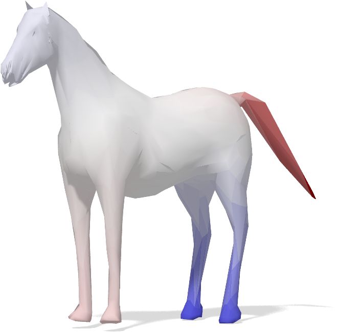
10                                         E. Rodolà et al. / Functional Maps Representation on Product Manifolds

[Fie73] F IEDLER M.: Algebraic connectivity of graphs. Czechoslovak             [OBCS∗ 12] OVSJANIKOV M., B EN -C HEN M., S OLOMON J.,
   Math. J. 23, 98 (1973), 298–305. 3                                             B UTSCHER A., G UIBAS L.: Functional maps: a flexible repre-
[GO17] G LASHOFF K., O RTLIEB C. P.: Composition operators, matrix                sentation of maps between shapes. ACM Trans. Graph. 31, 4 (July
  representation, and the finite section method: A theoretical framework          2012), 30:1–30:11. 3, 4, 5
  for maps between shapes. arXiv:1705.00325 (2017). 5                           [OCB∗ 17] OVSJANIKOV M., C ORMAN E., B RONSTEIN M., RODOLÀ
[GP10] G UILLEMIN V., P OLLACK A.: Differential Topology. AMS                     E., B EN -C HEN M., G UIBAS L., C HAZAL F., B RONSTEIN A.: Com-
  Chelsea Publishing Series. American Mathematical Soc., 2010. 2                  puting and processing correspondences with functional maps. In ACM
                                                                                  SIGGRAPH 2017 Courses (2017), pp. 5:1–5:62. 1, 2, 5
[GRS10] G RÖCHENIG K., R ZESZOTNIK Z., S TROHMER T.: Conver-
  gence analysis of the finite section method and banach algebras of ma-        [PBB∗ 13] P OKRASS J., B RONSTEIN A. M., B RONSTEIN M. M.,
  trices. Integral Equations and Operator Theory 67, 2 (2010), 183–202.           S PRECHMANN P., S APIRO G.: Sparse modeling of intrinsic correspon-
  5                                                                               dences. Computer Graphics Forum 32, 2 (2013), 459–468. 1
[HIK11] H AMMACK R., I MRICH W., K LAVZAR S.: Handbook of prod-                 [PM90] P ERONA P., M ALIK J.: Scale-space and edge detection using
  uct graphs, second ed. CRC Press, 2011. 3, 8                                    anisotropic diffusion. IEEE Trans. Pattern Anal. Mach. Intell. 12, 7 (July
                                                                                  1990), 629–639. 6
[HO17] H UANG R., OVSJANIKOV M.: Adjoint map representation for
  shape analysis and matching. Computer Graphics Forum 36, 5 (2017),            [RCB∗ 17] RODOLÀ E., C OSMO L., B RONSTEIN M. M., T ORSELLO
  151–163. 1                                                                      A., C REMERS D.: Partial functional correspondence. Computer Graph-
                                                                                  ics Forum 36, 1 (2017), 222–236. 2
[HWG14] H UANG Q., WANG F., G UIBAS L.: Functional map networks
  for analyzing and exploring large shape collections. ACM Transactions         [Sch83] S CHLEGEL V.:       Theorie der homogen zusammengesetzten
  on Graphics (TOG) 33, 4 (2014), 36. 1                                            Raumgebilde. Nova Acta, Ksl. Leop.-Carol. Deutsche Akademie der
                                                                                   Naturforscher, Band XLIV, Nr. 4, Druck von E. Blochmann und Sohn,
[KBB∗ 13] KOVNATSKY A., B RONSTEIN M. M., B RONSTEIN A. M.,                        Dresden, 1883. 4
  G LASHOFF K., K IMMEL R.: Coupled quasi-harmonic bases. Computer
  Graphics Forum 32, 2 (2013), 439–448. 1                                       [SGB13] S OLOMON J., G UIBAS L., B UTSCHER A.: Dirichlet energy
                                                                                  for analysis and synthesis of soft maps. Computer Graphics Forum 32,
[KBBV15]    KOVNATSKY A., B RONSTEIN M.         M., B RESSON X., VAN -            5 (2013), 197–206. 1, 8
     DERGHEYNST P.: Functional correspondence   by matrix completion. In
     Proc. CVPR (Boston, 2015), IEEE, pp. 905–914. 1                            [SK17] S HAMAI G., K IMMEL R.: Geodesic distance descriptors. In
                                                                                  Proc. CVPR (Honolulu, 2017), IEEE. 1
[KGB16] KOVNATSKY A., G LASHOFF K., B RONSTEIN M. M.:
  MADMM: a generic algorithm for non-smooth optimization on mani-               [SNB∗ 12] S OLOMON J., N GUYEN A., B UTSCHER A., B EN -C HEN M.,
  folds. In Proc. ECCV (Amsterdam, 2016), Springer. 1                             G UIBAS L.: Soft maps between surfaces. Computer Graphics Forum
                                                                                  31, 5 (2012), 1617–1626. 1, 2
[Lav17] L AVENANT H.: Harmonic mappings valued in the Wasserstein
   space. arXiv:1712.07528 (2017). 8                                            [SPKS16] S OLOMON J., P EYRÉ G., K IM V. G., S RA S.: Entropic metric
[LRB∗ 16] L ITANY O., RODOLÀ E., B RONSTEIN A. M., B RONSTEIN                     alignment for correspondence problems. ACM Transactions on Graphics
  M. M., C REMERS D.: Non-rigid puzzles. Computer Graphics Forum                  (TOG) 35, 4 (2016), 72:1–72:13. 1
  35, 5 (2016), 135–143. 2                                                      [Tu11] T U L. W.: An Introduction to Manifolds, second ed. Springer-
[LRR∗ 17] L ITANY O., R EMEZ T., RODOLÀ E., B RONSTEIN A. M.,                      Verlag New York, 2011. 2
  B RONSTEIN M. M.: Deep functional maps: Structured prediction for             [VLB∗ 17] V ESTNER M., L ÄHNER Z., B OYARSKI A., L ITANY O.,
  dense shape correspondence. In Proceedings of the IEEE International            S LOSSBERG R., R EMEZ T., RODOLÀ E., B RONSTEIN A., B RONSTEIN
  Conference on Computer Vision (Venice, 2017), vol. 2, IEEE, pp. 5660–           M., K IMMEL R., C REMERS D.: Efficient deformable shape correspon-
  5668. 2                                                                         dence via kernel matching. In Proceedings - 2017 International Confer-
[LRS∗ 16] L ÄHNER Z., RODOLÀ E., S CHMIDT F. R., B RONSTEIN                       ence on 3D Vision, 3DV 2017 (Qingdao, 2017), IEEE, pp. 517–526. 1,
  M. M., C REMERS D.: Efficient globally optimal 2D-to-3D deformable              7
  shape matching. In Proceedings of the IEEE Computer Society Confer-           [VLR∗ 17] V ESTNER M., L ITMAN R., RODOLÀ E., B RONSTEIN A.,
  ence on Computer Vision and Pattern Recognition (Las Vegas, 2016),              C REMERS D.: Product manifold filter: Non-rigid shape correspondence
  IEEE, pp. 2185–2193. 1                                                          via kernel density estimation in the product space. In Proceedings - 30th
[MCSK∗ 17] M ANDAD M., C OHEN -S TEINER D., KOBBELT L., A L -                     IEEE Conference on Computer Vision and Pattern Recognition, CVPR
  LIEZ P., D ESBRUN M.: Variance-minimizing transport plans for inter-            2017 (Honolulu, 2017), IEEE, pp. 6681–6690. 1, 7
  surface mapping. ACM Transactions on Graphics 36, 4 (2017), 39:1–             [WGBS18] WANG L., G EHRE A., B RONSTEIN M. M., S OLOMON J.:
  39:14. 1                                                                        Kernel functional maps. Computer Graphics Forum 37, 5 (2018), 27–
[Mém11] M ÉMOLI F.: Gromov–Wasserstein Distances and the Metric                   36. 1
  Approach to Object Matching. Foundations of computational mathe-              [Wit83] W ITKIN A. P.: Scale-space filtering. In Proceedings of the
  matics 11, 4 (2011), 417–487. 1                                                 Eighth International Joint Conference on Artificial Intelligence - Vol-
[MRCB18] M ELZI S., RODOLÀ E., C ASTELLANI U., B RONSTEIN M.:                     ume 2 (San Francisco, CA, USA, 1983), IJCAI’83, Morgan Kaufmann
  Localized manifold harmonics for spectral shape analysis. Computer              Publishers Inc., pp. 1019–1022. 6
  Graphics Forum 37, 6 (2018), 20–34. 1, 5, 6                                   [WSSC11] W INDHEUSER T., S CHLICKEWEI U., S CHMIDT F. R., C RE -
[NBH18] NASIKUN A., B RANDT C., H ILDEBRANDT K.: Fast approx-                     MERS D.: Geometrically consistent elastic matching of 3d shapes: A
  imation of laplace–beltrami eigenproblems. Computer Graphics Forum              linear programming solution. In Proc. ICCV (Barcelona, 2011), IEEE. 1
  37, 5 (2018), 121–134. 8                                                      [ZWW∗ 10] Z ENG Y., WANG C., WANG Y., G U X., S AMARAS D.,
[NMR∗ 18] N OGNENG D., M ELZI S., RODOLÀ E., C ASTELLANI U.,                      PARAGIOS N.: Dense non-rigid surface registration using high-order
  B RONSTEIN M., OVSJANIKOV M.: Improved functional mappings via                  graph matching. In Proc. CVPR (San Francisco, 2010), IEEE. 1
  product preservation. Computer Graphics Forum 37, 2 (2018), 179–190.
  1
[NO17] N OGNENG D., OVSJANIKOV M.: Informative descriptor preser-
  vation via commutativity for shape matching. Computer Graphics Forum
  36, 2 (2017), 259–267. 1

                                                                                                                submitted to COMPUTER GRAPHICS Forum (1/2019).
You can also read