Generating and Eroding Fractal Terrain for SimCity 4
←
→
Page content transcription
If your browser does not render page correctly, please read the page content below
David Coats
Scientific Computing
Final Report
May 2nd, 2008
Generating and Eroding Fractal Terrain for SimCity 4
1. Introduction:
Computer games need landscapes. Across genres of computer games, the
landscape in which game play occurs is an integral part of the game experience. The role
of the landscape can vary from first person shooters like Halo where levels are designed
specifically to provide a challenging combat arena, to simulation games like SimCity
where a realistic landscape is the starting point of the game. I investigate the generation
of landscapes for this simulation type of game.
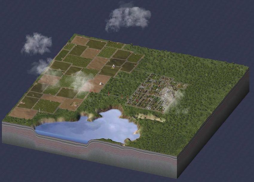
Figure 1: A quiet farming town situated on a bay in SimCity4. Who knows what
fantastic possibilities await this hamlet.
In these simulation games bigger is better for the landscape. The larger the
environment one can build on, the more satisfying the game experience. But these large
landscapes are tiresome to construct by hand using in game tools and worse, as shown in
Figure 2 these handcrafted landscapes retain distinctly unnatural artifacts.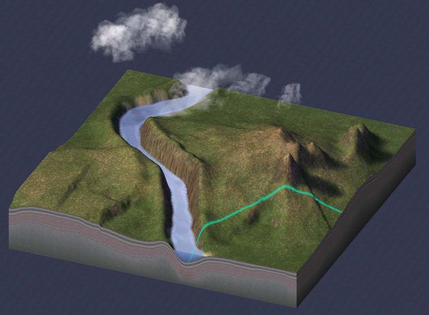
Figure 2: Landscape created using in-game mountain, mesa, canyon, cliff, flatten
       and fault tools. Visible is the area of effect indicator for a landscape editing tool. The
       landscape looks artificial.

        To remedy these time and quality drawbacks, an automatic routine that will create
qualitatively realistic landscapes is desired. While fractals had been noticed near the
beginning of the 20th century, the fractal nature of landscapes was first noted by Benoit
Mandelbrot when he viewed a ridgeline silhouetted by sunset (Musgrave 2004). Since the
inclusion of stochastic processes to remove the perfect self-similarity characteristic of
fractals computer terrain generation has been dominated by fractal methods, especially
discrete fractal methods. While these methods can quickly generate startlingly realistic
landscapes, discrete fractals usually exhibit unnaturally exaggerated roughness as shown
in Figure 3.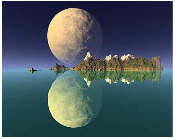
Figure 3: A fractal silhouette. Blessed State, 1988 by Kenton Musgrave.

        The missing element in fractal terrain is the smoothing process of erosion by
water. Fractals can be generated by any number of means, and the use of continuous basis
functions has allowed this smoothing to be simulated in the fractal creation itself. These
continuous basis functions are usually derived from noise functions. The noise functions
themselves produce noise with a particular frequency power spectrum that can be
controlled. The fractal dimension, or roughness of the fractal, is varied between each
level of fractal iteration, or octave, by increasing the frequency composition of the higher
octave by a value called the lacunarity of the fractal. Consequently, the ever finer small
scale features of the fractal landscape are made by increasing the power contained in high
frequency components of the noise function. The Perlin basis function is often used, and
the properties of the above terms are illustrated with regard to the Perlin basis function in
Musgrave 2004.

       (I want to do some generation with the Perlin basis function)

        While this continuous approach has shown success in generating apparently
eroded landscapes (Musgrave 2004), river networks, meandering streams and fluvial
plains are features have not been adequately reproduced using fractals. These features are
produced by applying a model of hydraulic erosion to the previously generated fractal
landscape. These models replicate the effects of rainfall by using ‘raindrops’ that begin
somewhere on the landscape then travel downhill while eroding and/or depositing
volume in the positions they pass through.

        The final step of landscape generation is rendering. This final step involves
coloring the landscape perhaps based on steepness or elevation above sea-level,
ray-tracing or otherwise forming a perspective view of the landscape, and finally adding
finishing touches like atmospheric haze. For this project the rendering capabilities of
SimCity 4 were used. The three step process of generation, erosion, and rendering is
shown in Figure 4.

       Figure 4: Landscape creation process. The top image is the fractal generated
       terrain. The middle image is the terrain after erosion. The bottom image is the fully
       rendered landscape.

2.      Methods:
        MATLAB was used as the coding environment for fractal terrain generation and
erosion. The eroded landscape was scaled to cover the range of values 0 to 255, then each
values was rounded to the nearest integer. With the data cover the range of unsigned 8-bit
integers, the data could be exported to a gray-scale bitmap. Within SimCity 4, at the
“region” screen pressing CTRL-SHFT-ALT-R will bring up a browser that allows the
gray-scale bitmap to be loaded.

2.1    Fractal Generation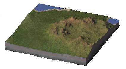
(Two?) fractal generation schemes were used: the diamond-square algorithm (and
the considerably more complex Perlin noise basis function?). The diamond-square
algorithm operates according to Figure 5 and was used the following parameters.

       Figure 5: The diamond square algorithm. Frame a shows the initial seeding. Frames
       b and c show one iteration, and frames d and e show a second iteration of the
       algorithm.

Random number distribution – Uniform probability over the unit interval (-0.5 to 0.5).

Stochastic parameter – 0.2.

        The diamond-square algorithm creates square terrains which have sizes of 2i + 1,
where i is the number of iterations desired. The algorithm begins by seeding the
outermost corners of an array with random values drawn from the chosen random number
distribution. In the first iteration, the average of the neighboring corner values is
computed, then to this average is added a value drawn from the random number
distribution which has been scaled by the product of the average and the stochastic
parameter. The midpoints of the square are then similarly filled using neighboring values.
This creates four new squares, and the process proceeds with the second iteration. This
generation scheme is O(n2), where n is the size of landscape generated as shown in Figure
6.

       Figure 6: Log-Log plot of diamond-square algorithm runtime for various landscape
       sizes.

       (Perlin basis function discussion?)

2.2     Erosion Methods
        (Two?) ad hoc hydraulic erosion methods were tried and there key features are
best described functionally:

One-to-one Volume Transport
Raindrop generation – Uniform probability for each vertex over whole surface.

Raindrop Travel – From the vertex of generation, the raindrop moves to whichever of its
eight nearest neighboring vertices has the lowest height value.
Sediment Pick-up –At each position visited a 0.2 probability exists that the raindrop will
collect sediment. The amount of sediment collected by the raindrop is determined by
choosing a value with uniform probability from the unit interval (0,1), then multiplying
the height of the current position by 0.2 times this random value. This means a maximum
of 1/5th the height of the current position can be eroded by a raindrop. The height of the
current position is decreased by the calculated value and the volume corresponding to this
decrease in height is transported away by the raindrop.
Sediment Deposition – The raindrop travels downhill by moving to the lowest of its eight
grid neighbors. When no lower neighbor is found, or the edge of the map has been
reached, then the height of the current position is adjusted to according to conservation of
volume.
This method is roughly O(n), where n is the number of raindrops.
Continuous, Gradient Dependent Erosion
Instead of using raindrops, this approach uses a volume of water that moves over the
landscape between vertices and over the course of many time steps (based on Musgrave
1989).
Rainfall generation – Uniform amount of water is allowed to fall evenly over the
landscape (and linearly proportional to altitude) every 160 timesteps. This is represented
by increase the volume of water present at each vertex v at time step t, wtv, by an amount
rf .
Rainfall Travel and Sediment Pick-up – At each time step for each vertex, the amount of
water passed, ∆w, to each neighboring vertex u, having altitude atu, starting with the
lowest of the eight neighboring vertices, is defined as:
( )
∆w = min wtv , ( wtv + atv ) − ( wtu + atu ) .
If ∆w is less than or equal to zero, an amount of sediment, st+1v, is deposited at the vertex
for the next time step. The altitude of the vertex and the sediment carried in the water
covering the vertex are adjusted for the next time step according to:
a tv+1 = a tv + K d s tv
stv+1 = (1 − K d ) s tv
If ∆w is greater than zero, the water volume at vertex v is decreased and the water volume
at the neighbor vertex u is increased by ∆w. The water carries with it an amount of
sediment cs that is subtracted from the sediment available at the vertex. If stv > cs, then the
sediment is adjusted according to:c s = K c ∆w
stv+1 = s tv − c s .
stu+1 = s tu + c s
But if over the course of updating the neighboring vertices, stv < cs, extra sediment is
eroded from the height of the current vertex according to:
stv+1 = 0
stu+1 = stu + s tv + K s (c s − stv ) .
a tv+1 = atv − K s (c s − s tv )
If sediment remains in the current vertex after the sediment demands of water flows to its
neighbors are met, then the altitude of the vertex is increased as some of the sediment is
deposited:
a tv+1 = a tv + K d s tv
.
stv+1 = s tv − K d s tv
The constants Kc, Kd, and Ks are respectively the sediment capacity, sediment deposition
and soil softness constants.
3. Geometry
The geometry of the surface considered deserves special attention. The surface of the
landscape is approximated by many planar sections each formed between exactly three
vertices as shown in Figure 7.
Figure 7: The landscape surface is approximated using many planar sections that
make up formed between triplets of vertices. (needs to be pyramidized)To calculate the volume under this surface we can divide the surface into eight volumes
each with a triangular top plane. The volume beneath each of these surfaces can be seen
as the triangular base area times the average height of the top plane. Because the top
plane is triangular its average height is simply the average of the three vertex heights.
Thus if the bottom is a right isosceles triangle with side length d, the volume beneath one
of the triangular patches is:
d2
V patch = (h1 + h2 + h3 ) .
6
The volume of the pyramid-like shape in terms of the vertex heights is then:
d2 1 1
V=
6
o
8 h + 2 ∑ ∑ hIJ .
i = −1,i ≠ 0 j = −1, j ≠ 0
Of interest to relating heights to volumes of deposition and erosion is the volume
generated by a difference in h0 from initial and final values:
8d 2
∆V = V (hi ) − V (h f ) = (hi − h f ) .
6
This is a fortuitous conclusion, since it means that volume can be conserved simply
conserving height. Note that this is a special property of this type of surface alone.
References:
Sutherland, Ben. Particle Based Enhancement of Terrain Data. ACM SIGGRAPH 2006
Research Posters. Article No. 96, 2006.
Musgrave, Kenton F. The Synthesis and Rendering of Eroded Fractal Terrains. Computer
Graphics. vol. 23, no. 3, pgs. 41-50, July 1989.
Musgrave, Kenton F. Fractal Terrains and Fractal Planets. ACM SIGGRAPH 2004
Course Notes. Article No. 32, 2004.
Appendix A: Source Code
function [land3 land2] = createErodedLand(m,n)
%By David Coats, Apr 2008, david.coats@gmail.com
%
%This function is meant to create an eroded land. It takes in the m x n
%size of the land you want to generate, using these parameters to call
%createFractalLand for a square that would be large enough to cut out
the%m x n portion desired.
%
%Then the land is eroded.
tic
%Parameters
deposProb = 0;
erodeProb = 0.2;
erodeVal = 0.2;
raindrops = 500000;
frameRate = 1000;
%Create a fractal land
land = createFractalLand(ceil(log2(max(m, n))));
%Cut the land down to the size we want
land = land(1:m,1:n);
display(strcat(['Fractal land generated in ',num2str(toc),'
seconds.']));
%Get the max height of this land for viewing purposes
height = max(land(:));
%Create a copy of the initial land to see changes
land2 = land;
%land2 = land;
%For movie creation
count = 1;
hold off;
%Now we erode via isochoric raindrops.
for i = 1:raindrops
%choose a random land tile
M = ceil(m*rand);
N = ceil(n*rand);
%By a strange coincidence, the change in volume is equal to 4/3 the
%change in height. Who knew? What this does is move downhill until
the
%raindrop picks up a portion of volume. Then, the volume is
deposited
%at the lowest point.
%Now we need to find a place from which to take volume.
x = M;
y = N;
stopper = 1;
stopper2 = 1;
while stopper;
for j = -1:1
for k = -1:1
if 0 < j+M && j+Mend
if x == M && N == y
stopper = 0;
stopper2 = 0;
else
M = x;
N = y;
if rand < erodeProb
dHeight = abs(land(M,N)* erodeVal * rand);
land(M,N) = land(M,N) - dHeight;
stopper = 0;
end
end
end
%Now we just need to find the proper place to deposit the height.
x = M;
y = N;
while stopper2;
for j = -1:1
for k = -1:1
if 0 < j+M && j+M% display(strcat(['The count is: ',num2str(count),' out of
',num2str(raindrops/frameRate)]));
% end
end
display(strcat(['Erosion complete at ',num2str(toc),' seconds.']));
%Temporary Plotting code
land(1,1) = min(land2(:));
surf(land);
figure
surf(land2);
land3 = land;
%Post-processing of land
Min = abs(min(land(:)));
land = land + Min;
Max = max(land(:));
Max = 255/Max;
land = land*Max;
land = round(land);
%Now save as a grayscale
land = uint8(land);
imwrite(land,'eroded.bmp');
display(strcat(['Total time: ',num2str(toc),' seconds.']));
%movie2avi(F,'erosion');
end
%%%%%%%%%%%%%%%%%%%%%%%%%%%%%%%%%%%%%%%%%%%%%%%%%%
function land = createFractalLand(power)
%By David Coats, Mar 2008, david.coats@gmail.com
%
%This function is meant to implement the Diamond-Square algorithm for
%fractal land generation.
if power < 1
error('Power input argument must be an integer that is one or
greater!');
end
lsize = 2^power+1;
land = zeros(lsize);
%Parameters
decreaseScaleTot = 0.2;
height = 1;
%Setup the land corners.
land(1,1) = height*(rand-0.5);
land(end,1) = height*(rand-0.5);
land(1,end) = height*(rand-0.5);
land(end,end) = height*(rand-0.5);
%Use a queue to hold which points should be visited.step = (lsize - 1)/2;
Q = zeros(4,lsize^2 - 4);
Q(:,1) = [1 + step; 1+ step; 1; step]; %enqueue the middle point. Type
1 point means that lateral points are next.
count = 1;
qCount = 2;
while 1
%Breaking condition, should break before step gets to 0.25, minus
three
%due to corners.
if count == lsize^2 -3
break;
end
%Decrease scale mellows with time.
decreaseScale = decreaseScaleTot*step;
%Dequeue our current tile.
current = Q(:,count);
step = current(4);
%Here gets the last round of points
if step == 0.5
step = 1;
end
%Now many conditionals for enqueuing our points.
if current(3) == 1 %Then enqueue lateral points
if current(1) - step > 0
if land(current(1) - step, current(2)) == 0
temp = [current(1) - step; current(2); 2; step/2];
land(current(1) - step, current(2)) = 1;
Q(:,qCount) = temp;
qCount = qCount + 1;
end
end
if current(1) + step 0
if land(current(1), current(2) - step) == 0
temp = [current(1); current(2) - step; 2; step/2];
land(current(1), current(2) - step) = 1;
Q(:,qCount) = temp;
qCount = qCount + 1;
end
end
if current(2) + stepif land(current(1), current(2) + step) == 0
temp = [current(1); current(2) + step; 2; step/2];
land(current(1), current(2) + step) = 1;
Q(:,qCount) = temp;
qCount = qCount + 1;
end
end
%Now create the current point's elevation
sum = 0;
n = 0;
if current(1) - step > 0 && current(2) - step > 0
sum = sum + land(current(1) - step, current(2) - step);
n = n + 1;
end
if current(1) + step 0 && current(1) + step 0 && current(2) - step > 0
if land(current(1) - step, current(2) - step) == 0
temp = [current(1) - step; current(2) - step; 1; step];
land(current(1) - step, current(2) - step) = 1;
Q(:,qCount) = temp;
qCount = qCount + 1;
end
end
if current(1) + step 0 && current(1) + stepQ(:,qCount) = temp;
qCount = qCount + 1;
end
end
if current(2) + step 0
if land(current(1) - step, current(2) + step) == 0
temp = [current(1) - step; current(2) + step; 1; step];
land(current(1) - step, current(2) + step) = 1;
Q(:,qCount) = temp;
qCount = qCount + 1;
end
end
%Now create the current point's elevation
sum = 0;
n = 0;
if current(1) - 2*current(4) > 0
sum = sum + land(current(1) - 2*current(4), current(2));
n = n + 1;
end
if current(1) + 2*current(4) 0
sum = sum + land(current(1), current(2) - 2*current(4));
n = n + 1;
end
if current(2) + 2*current(4)You can also read