HB-PLS: A statistical method for identifying biological process or pathway regulators by integrating Huber loss and Berhu penalty with partial ...
←
→
Page content transcription
If your browser does not render page correctly, please read the page content below

ARTICLE
                                                                                                                     https://doi.org/10.48130/FR-2021-0006
                                                                                                                                  Forestry Research 2021, 1: 6

HB-PLS: A statistical method for identifying biological process or
pathway regulators by integrating Huber loss and Berhu penalty with
partial least squares regression
Wenping Deng1, Kui Zhang2, Cheng He3, Sanzhen Liu3, and Hairong Wei1*
1 College of Forest Resources and Environmental Science, Michigan Technological University, Houghton, Michigan 49931, United States of America
2 Department of Mathematical Science, Michigan Technological University, Houghton, Michigan 49931, United States of America
3 Department of Plant Pathology, Kansas State University, Manhattan, Kansas 66506, United States of America

* Corresponding author, E-mail: hairong@mtu.edu

    Abstract
    Gene expression data features high dimensionality, multicollinearity, and non-Gaussian distribution noise, posing hurdles for identification of
    true regulatory genes controlling a biological process or pathway. In this study, we integrated the Huber loss function and the Berhu penalty (HB)
    into partial least squares (PLS) framework to deal with the high dimension and multicollinearity property of gene expression data, and developed
    a new method called HB-PLS regression to model the relationships between regulatory genes and pathway genes. To solve the Huber-Berhu
    optimization problem, an accelerated proximal gradient descent algorithm with at least 10 times faster than the general convex optimization
    solver (CVX), was developed. Application of HB-PLS to recognize pathway regulators of lignin biosynthesis and photosynthesis in Arabidopsis
    thaliana led to the identification of many known positive pathway regulators that had previously been experimentally validated. As compared to
    sparse partial least squares (SPLS) regression, an efficient method for variable selection and dimension reduction in handling multicollinearity,
    HB-PLS has higher efficacy in identifying more positive known regulators, a much higher but slightly less sensitivity/(1-specificity) in ranking the
    true positive known regulators to the top of the output regulatory gene lists for the two aforementioned pathways. In addition, each method
    could identify some unique regulators that cannot be identified by the other methods. Our results showed that the overall performance of HB-
    PLS slightly exceeds that of SPLS but both methods are instrumental for identifying real pathway regulators from high-throughput gene
    expression data, suggesting that integration of statistics, machine leaning and convex optimization can result in a method with high efficacy and
    is worth further exploration.

    Citation: Deng W, Zhang K, He C, Liu S, Wei H. 2021. HB-PLS: A statistical method for identifying biological process or pathway regulators by
    integrating Huber loss and Berhu penalty with partial least squares regression. Forestry Research 1: 6 https://doi.org/10.48130/FR-2021-0006

INTRODUCTION                                                                       stochastic networks[3], Bayesian[4,5] or dynamic Bayesian
                                                                                   networks (BN)[6,7], and ordinary differential equations (ODE)[8].
   In a gene regulatory network (GRN), a node corresponds to                       Some of these methods require time series datasets with
a gene and an edge represents a directional regulatory
                                                                                   short time intervals, such as those generated from easily
relationship between a transcription factor (TF) and a target
                                                                                   manipulated single cell organisms (e.g. bacteria, yeast etc.) or
gene. Understanding the regulatory relationships among
                                                                                   mammalian cell lines[9]. For this reason, most of these
genes in GRNs can help elucidate the various biological pro-
                                                                                   methods are not suitable for gene expression data, especially
cesses and underlying mechanisms in a variety of organisms.
                                                                                   time series data involving time intervals on the scale of days,
Although experiments can be conducted to acquire evidence
                                                                                   from multicellular organisms like plants and mammals
of gene regulatory interactions, these are labor-intensive and
time-consuming. In the past two decades, the advent of high-                       (except cell lines).
throughput technologies including microarray and RNA-Seq,                             In general, the methods that are useful for building gene
have generated an enormous wealth of transcriptomic data.                          networks with non-time series data generated from higher
As the data in public repositories grows exponentially, com-                       plants and mammals include ParCorA[10], graphical Gaussian
putational algorithms and tools utilizing gene expression                          models (GGM)[11], and mutual information-based methods
data offer a more time- and cost-effective way to reconstruct                      such as Relevance Network (RN)[12], Algorithm for the
GRNs. To this end, efficient mathematical and statistical                          Reconstruction of Accurate Cellular Networks (ARACNE)[13],
methods are needed to infer qualitative and quantitative                           C3NET[14], maximum relevance/minimum redundancy
relationships between genes.                                                       Network (MRNET)[15], and random forests[16,17]. Most of these
   Many methods have been developed to reconstruct GRNs,                           methods are based on the information-theoretic framework.
each employing different theories and principles. The earliest                     For instance, Relevance Network (RN)[18], one of the earliest
methods include differential equations[1], Boolean networks[2],                    methods developed, infers a network in which a pair of genes
                                                                                                                                  www.maxapress.com/forres
© The Author(s)                                                                                                                       www.maxapress.com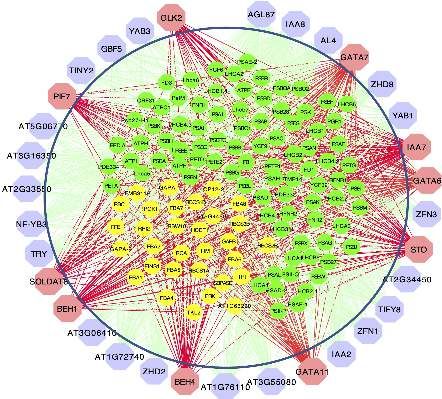
Huber-Berhu partial least squares regression

                                                                                            ∑p
are linked by an edge if the mutual information is larger than                    P (β) =    j=1 β j
                                                                                                  2,   on the coefficients which introduces a bias but
a given threshold. The context likelihood relatedness (CLR)                       reduces the variance of the estimated, β̂ . In ridge regression,
algorithm[19], an extension of RN, derives a score from the                       there is a unique solution even for the p > n case. Least absolute
empirical distribution of the mutual information for each pair                    shrinkage and selection operator (LASSO)[27] is similar to ridge
of genes and eliminates edges with scores that are not                            regression, except the ℓ2 penalty in ridge regression is replaced
statistically significant. ARACNE is similar to RN; however,                                                ∑
                                                                                  by the ℓ1 penalty, P (β) = pj=1 β j .
ARACNE makes use of the data processing inequality (DPI) to
eliminate the least significant edge of a triplet of genes, which                     The main benefit of least absolute shrinkage and selection
decreases the false positive rate of the inferred network.                        operator (LASSO) is that it performs variable selection and
MRNET[20] employs the maximum relevance and minimum                               regularization simultaneously thereby generating a sparse
redundancy feature selection method to infer GRNs. Finally,                       solution, a desirable property for constructing GRNs. When
triple-gene mutual interaction (TGMI) uses condition mutual                       LASSO is used for selecting regulatory TFs for a target gene,
information to evaluate triple gene blocks to infer GRNs[21].                     there are two potential limitations. First, if several TF genes
Information theory-based methods are used extensively for                         are correlated and have large effects on the target gene,
constructing GRNs and for building large networks because                         LASSO has a tendency to choose only one TF gene while
they have a low computational complexity and are able to                          zeroing out the other TF genes. Second, some studies[28] state
capture nonlinear dependencies. However, there are also                           that LASSO does not have oracle properties; that is, it does
disadvantages in using mutual information, including high                         not have the capability to identify the correct subset of true
false-positive rates[22] and the inability to differentiate                       variables or to have an optimal estimation rate. It is claimed
positive (activating), negative (inhibiting), and indirect                        that there are cases where a given λ that leads to optimal
regulatory relationships. Reconstruction of the transcriptional                   estimation rate ends up with an inconsistent selection of
regulatory network can be implemented by the neighbor-                            variables. For the first limitation, Zou and Hastie[29] proposed
hood selection method. Neighborhood selection[23] is a sub-                       elastic net, in which the penalty is a mixture of LASSO and
                                                                                                                      ∑              ∑p 2
problem of covariance selection. Assume Γ is a set containing                     ridge regressions: P (β) = α pj=1 β j + 1−α     2    j=1 β j ,
                                                                                                                                                      where
all of the variables (genes), the neighborhood nea of a variable                  α(0 < α < 1) is called the elastic net mixing parameter. When
a ∈ Γ is the smallest subset of Γ\ {a} such that, given all                       α = 1 , the elastic net penalty becomes the LASSO penalty;
variables in nea , variable a is conditionally independent of all                 when α = 0 , the elastic net penalty becomes the ridge
remaining variables. Given n i.i.d. observations of Γ , neighbor-                 penalty. For the second limitation, adaptive LASSO[28] was
hood selection aims to estimate the neighborhood of each                          proposed as a regularization method, which enjoys the oracle
variable in Γ individually. The neighborhood selection                            properties. The penalty function for adaptive LASSO is:
                                                                                            ∑
problem can be cast as a multiple linear regression problem                       P (β) = pj=1 ŵ j β j , where adaptive weight ŵ j = 1 γ , and
and solved by regularized methods.                                                                                                           |β̂ini |
   Following the differential equation in[24], the expression                      β̂ini is an initial estimate of the coefficients obtained through
levels of a target gene y and the expression levels of the TF                     ridge regression or LASSO; γ is a positive constant, and is
genes x form a linear relationship:                                               usually set to 1. It is evident that adaptive LASSO penalizes
                                                                                  more those coefficients with lower initial estimates.
                    yi = β0 + xiT β + εi i = 1, 2, . . . , n                (1)
                                                                                      It is well known that the square loss function is sensitive to
where n is the number of samples, xi = (xi1 , . . . , xip )T is the               heavy-tailed errors or outliers. Therefore, adaptive LASSO may
expression level of p TF genes, and yi is the expression level of                 fail to produce reliable estimates for datasets with heavy-
the target gene in sample i. β0 is the intercept and                              tailed errors or outliers, which commonly appear in gene
β = (β1 , · · · , β p )T are the associated regression coefficients; if any       expression datasets. One possible remedy is to remove
β j , 0 ( j = 1, · · · , p), then TF gene j regulates target gene i. {εi }        influential observations from the data before fitting a model,
are independent and identically distributed random errors with                    but it is difficult to differentiate true outliers from normal
mean 0 and variance σ2 . The method to get an estimate of β                       data. The other method is to use robust regression. Wang et
and β0 is to transform this statistical problem to a convex                       al.[30] combined the least absolute deviation (LAD) and
optimization problem:                                                             weighted LASSO penalty to produce the LAD-LASSO method.
                                    ∑n          (               )
   β = argminβ f (β) = argminβ                 L yi − β0 − xiT β + λP (β)   (2)   The objective function is:
                                         i=1                                                       ∑n                             ∑p
                                                                                                               yi − β0 − xiT β + λ   ŵ j β j           (3)
where L(·) is a loss function, P(·) is a penalization function, and                                      i=1                        j=1
λ > 0 is a tuning parameter which determines the importance of                       With this LAD loss, LAD-LASSO is more robust than OLS to
penalization. Different loss functions, penalization functions,                   unusual y values, but it is sensitive to high leverage outliers.
and methods for determining λ have been proposed in the                           Moreover, LAD estimation degrades the efficiency of the
literature. Ordinary least squares (OLS) is the simplest method                   resulting estimation if the error distribution is not heavy
                                                                   2
with a square loss function L(yi − β0 − xiT β) = (yi − β0 − xiT β)                tailed[31]. To achieve both robustness and efficiency, Lambert-
and no penalization function. The OLS estimator is unbiased[25].                  Lacroix and Zwald 2011[32], proposed Huber-LASSO, which
However, since it is common for the number of genes, p, to be                     combined the Huber loss function and a weighted LASSO
much larger than the number of samples, n, (i.e. p ≫ n) in any                    penalty. The Huber function (see Materials and Methods) is a
given gene expression data set, there is no unique solution for                   hybrid of squared error for relatively small errors and absolute
OLS. Even when n > p , OLS estimation features high variance.                     error for relatively large ones. Owen 2007[33] proposed the use
To tackle these problems, ridge regression[26] adds a ℓ2 penalty,                 of the Huber function as a loss function and the use of a

Page 2 of 13                                                                                                        Deng et al. Forestry Research 2021, 1: 6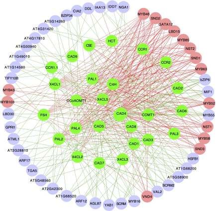
Huber-Berhu partial least squares regression
reversed version of Huber’s criterion, called Berhu, as a normalized with the robust multi-array analysis (RMA)
penalty function. For the Berhu penalty (see Materials and algorithm in affy package. This compendium data set was also
Methods), relatively small coefficients contribute their ℓ1 norm used in our previous studies[40]. The maize B73 compendium
to the penalty while larger ones cause it to grow quadra- data set used for predicting photosynthesis light reaction
tically. This Berhu penalty sets some coefficients to 0, like (PLR) pathway regulators was downloaded from three NCBI
LASSO, while shrinking larger coefficients in the same way as databases: (1) the sequence read archive (SRA)
ridge regression. In[34], the authors showed that the combi- (https://www.ncbi.nlm.nih.gov/sra), 39 leaf samples from
nation of the Huber loss function and an adaptive Berhu ERP011838; (2) Gene Expression Omnibus (GEO), 24 leaf
penalty enjoys oracle properties, and they also demonstrated samples from GSE61333, and (3) BioProject (https://www.
that this procedure encourages a grouping effect. In previous ncbi.nlm.nih.gov/bioproject/), 36 seedling samples from
research, the authors solved a Huber-Berhu optimization PRJNA483231. This compendium is a subset of that used in
problem using CVX software[33−35], a Matlab-based modeling our earlier co-expression analysis[41]. Raw reads were trimmed
system for convex optimization. CVX turns Matlab into a to remove adaptors and low-quality base pairs via
modeling language, allowing constraints and objectives to be Trimmomatic (v3.3). Clean reads were aligned to the B73Ref3
specified using standard Matlab expression syntax. However, with STAR, followed by the generation of normalized FPKM
since CVX is slow for large datasets, a proximal gradient (fragments per kb of transcript per million reads) using
descent algorithm was developed for the Huber-Berhu Cufflinks software (v2.1.1)[42].
regression in this study, which runs much faster than CVX. Huber and Berhu functions
Reconstruction of GRNs often involves ill-posed problems In estimating regression coefficients, the square loss
due to high dimensionality and multicollinearity. Partial least function is well suited if yi follows a Gaussian distribution, but
squares (PLS) regression has been an alternative to ordinary it gives a poor performance when yi follows a heavy-tailed
regression for handling multicollinearity in several areas of distribution or there are outliers. On the other hand, the least
scientific research. PLS couples a dimension reduction absolute deviation (LAD) loss function is more robust to
technique and a regression model. Although PLS has been outliers, but the statistical efficiency is low when there are no
shown to have good predictive performance in dealing with outliers in the data. The Huber function, introduced in[43], is a
ill-posed problems, it is not particularly tailored for variable combination of linear and quadratic loss functions. For any
selection. Sæbø et al. 2007[36] first proposed the soft- given positive real M (called shape parameter), the Huber
threshold-PLS (ST-PLS), in which the ℓ1 penalty is used for PLS function is defined as:
loading weights of multiple latent components. Such a {
z2 |z| ≤ M
method is especially applicable for classification and variable H M (z) = (4)
2M |z| − M 2 |z| > M
selection when the number of variables is greater than the
number of samples. Chun and Keleş 2010 [37] proposed a This function is quadratic for small z values but grows
similar sparse PLS regression for simultaneous dimension linearly for large values of z. The parameter M determines
reduction and variable selection. Both the methods from where the transition from quadratic to linear takes place
Sæbø et al. 2007 and Chun and Keleş 2010 used the same ℓ1 (Fig. 1a). In this study, the default value of M was set to be
penalty for PLS loading weights. Lê Cao et al. 2008[38] also one tenth of the interquartile range (IRQ), as suggested by[44].
proposed a sparse PLS method for variable selection when The Huber function is a smooth function with a derivative
integrating omics data. They added sparsity into PLS with a function:
{
LASSO penalization combined with singular value decompo- ′ 2z |z| ≤ M
HM (z) = (5)
sition (SVD) computation. In this study, the Huber loss 2M sign (z) |z| > M
function and the Berhu penalty function were embedded into The ridge regression uses the quadratic penalty on
a PLS framework. Real gene data was used to demonstrate regression coefficients, and it is equivalent to putting a
that this approach is applicable for the reconstruction of Gaussian prior on the coefficients. LASSO uses a linear penalty
GRNs. on regression coefficients, and this is equivalent to putting a
Laplace prior on the coefficients. The advantage of LASSO
MATERIALS AND METHODS over ridge regression is that it implements regularization and
variable selection simultaneously. The disadvantage is that, if
High-throughput gene expression data a group of predictors is highly correlated, LASSO picks only
The lignin pathway analysis used an Arabidopsis wood one of them and shrinks the others to zero. In this case, the
formation compendium dataset containing 128 Affymetrix prediction performance of ridge regression dominates the
microarrays pooled from six experiments (accession LASSO. The Berhu penalty function, introduced in Owen
identifiers: GSE607, GSE6153, GSE18985, GSE2000, GSE24781, 2007[33], is a hybrid of the quadratic penalty and LASSO. It
and GSE5633 in NCBI Gene Expression Omnibus (GEO) gives a quadratic penalty to large coefficients while giving a
(http://www.ncbi.nlm.nih.gov/geo/)). These datasets were linear penalty to small coefficients, as shown in Fig. 1b. The
originally obtained from hypocotyledonous stems under Berhu function is defined as:
short-day conditions known to induce secondary wood
|z| |z| ≤ M
2
formation[39]. The original CEL files were downloaded from BM (z) =
z + M2 (6)
|z| > M
GEO and preprocessed using the affy package in 2M
Bioconductor (https://www.bioconductor.org/) and then The shape parameter M was set to be the same as that in
Deng et al. Forestry Research 2021, 1: 6 Page 3 of 13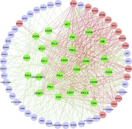
Huber-Berhu partial least squares regression

                a                         Huber loss                          b                           Berhu penalty
                                                                              4
                6

                5
                                                                              3
                4

                3                                                             2

                2
                                                                              1
                1

                0                                                             0
                    −3       −2      −1       0          1      2    3             −3     −2         −1        0          1        2       3

                c                     2D Huber contour                        d                      2D Berhu contour
                3                                                             3

                2                                                             2

                1                                                             1

                0                                                             0

               −1                                                            −1

               −2                                                            −2

               −3                                                            −3
                    −3       −2      −1       0          1      2    3             −3     −2         −1        0          1        2       3
  Fig. 1 Huber loss function (a) and Berhu penalty function (b); The 2D contours of Huber loss function (c) and Berhu penalty function (d).

the Huber function. As shown in Fig. 1b, the Berhu function is                a Huber_Berhu                b   LASSO                   c   Ridge
a convex function, but it is not differentiable at z = 0 . The 2D
                                                                                     β2                         β2                         β2
                                                                                     ^                          ^                           ^

contours of Huber and Berhu functions are shown in Fig. 1c
and Fig. 1d, respectively. When the Huber loss function and
the Berhu penalty were combined, an objective function, as
referred as the Huber-Berhu function, was obtained, as shown
below.                                                                                          β1
                                                                                                ^
                                                                                                                              β1
                                                                                                                              ^
                                                                                                                                                   β1
                                                                                                                                                   ^

                    ∑n                              ∑p   ( )
         f (β) =           H M (yi − β0 − xiT β) + λ   BM β j       (7)
                     i=1                           j=1

   The estimation of coefficients using the Huber-Berhu                           Fig. 2 Estimation picture for the Huber-Berhu regression (a)
objective (Fig. 2a), LASSO (Fig. 2b), and the ridge (Fig. 2c)                     when least absolute shrinkage and selection operator (LASSO)
regressions provided some insights. The Huber loss corres-                        (b) and ridge (c) regressions are used as a comparison.
ponds to the rotated, rounded rectangle contour in the top
right corner, and the center of the contour is the solution of                Berhu regression behaves like LASSO, which can generate a
the un-penalized Huber regression. The shaded area is a map                   sparse solution.
of the Berhu constraint where a smaller λ corresponds to a                    The algorithm to solve the Huber-Berhu regression
larger area. The estimated coefficient of the Huber-Berhu                        Since the Berhu function is not differentiable at z = 0 , it is
regression is the first place the contours touch the shaded                   difficult to use the gradient descent method to solve
area; when λ is small, the touch point is not on the axes,                    equation (4). Although we can use the general convex
which means the Huber-Berhu regression behaves more like                      optimization solver CVX[35] for a convex optimization
the ridge regression, which does not generate a sparse                        problem, it is too slow for real biological applications.
solution. When λ increases, the correspondent shaded area                     Therefore, a proximal gradient descent algorithm was
changes to a diamond, and the touch point is more likely to                   developed to solve equation (4). Proximal gradient descent is
be located on the axes. Therefore, for large λ , the Huber-                   an effective algorithm to solve an optimization problem with

Page 4 of 13                                                                                                   Deng et al. Forestry Research 2021, 1: 6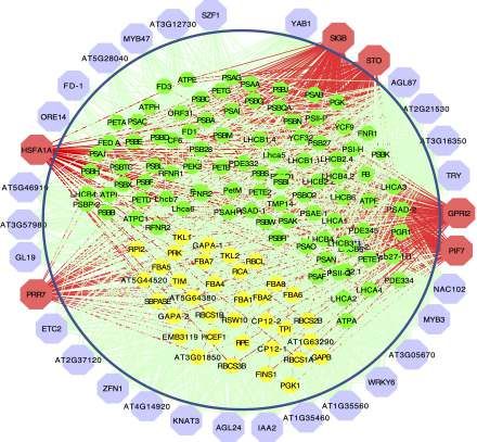
Huber-Berhu partial least squares regression
decomposable objective function. Suppose the objective Embedding the Huber-Berhu objective function into
function can be decomposed as f (z) = g (z) + h (z), where g (z) PLS
is a convex differentiable function and h (z) is a convex non- Let X(n × p) and Y(n × q) be the standardized predictor
differentiable function. The idea behind the proximal variables (gene expression of TF genes) and dependent
gradient descent[45] method is to make a quadratic variables (gene expression of pathway genes), respectively.
approximation to g (z) and leave h (z) unchanged. That is: PLS[48] looks for a linear combination of X and a linear
1 combination of Y such that their covariance reaches a
f (z) = g (z) + h (z) ≈ g (z) + ∇g(x)T (z − x) + ∥z − x∥22 + h (z) maximum:
2t
max∥u∥2 =1,∥v∥2 =1 cov (Xu, Yv) (11)
At each step, x is updated by the minimum of the right side of
above formula. Here, the linear combination ξ = Xu and η = Yv are called
component scores (or latent variables) which are generated
1
x+ = argminz g (x) + ∇g(z)T (z − x) + ∥z − x∥22 + h (z) through the p and q dimensional weight vectors u and v ,
2t
1 respectively. After getting this first component ξ , two
= argminz ∥z − (x − t∇g (x)∥22 + h (z) regression equations (from X to ξ and from Y to ξ ) were set
2t
1 up:
The operator Proxt,h (x) = argminz
|| z − x ||22 + h (z) is called X = ξc′ + ε1 , Y = ξd′ + ε2 = Xb + ε3 (12)
2t
proximal mapping for h. To solve (7), the key is to compute Here, c and d are commonly called loadings in the
the proximal mapping for the Berhu function: literature. Next, X was deflated as X = X − ξc′ and Y was
deflated as Y = Y − ξd′ , and this process was continued until
z2 + M 2 (| z| − M)2
λBM (z) = λ |z| 1|z|≤M + λ 1|z|>M = λ |z| + λ 1|z|>M enough components were extracted.
2M 2M
A close relationship exists between PLS and SVD. Let
2
let u (z) = λ (|z|−M)
2M 1|z|>M
. As u (z) satisfies theorem 4 in[46]: 1
M = X ′ Y , then cov (Xu, Yv) = u′ Mv . Let the SVD of M be:
n
Proxt,λB (x) = Proxt,λu (x) ◦ Proxt,λ|·| (x) (8)
M = U∆V ′
It is not difficult to verify: where U(p × r) and V(q × r) are orthonormal and ∆(r × r) is a
{ M } diagonal matrix whose diagonal elements δk (k = 1 . . . r) are
Proxt,λu (x) = sign (x) min |x| , (|x| + tλ) (9)
M + tλ called singular values. According to the property of SVD, the
combinatory coefficients u and v in (7) are exactly the first
Proxt,λ|·| (x) = sign (x) min {|x| − tλ, 0} (10) column of U and the first column of V . Therefore, the weight
vectors of PLS can be computed by:
Finding β0 and β that minimize f ( β) in (7) is detailed in
p
Algorithm 1. minu,v M − uv′ F
∑ p ∑q ( )2
Algorithm 1: Accelerated proximal gradient descent method to where ∥M − uv′ ∥Fp = i=1 j=1 mi j − ui v j
.
minimize f (β) in equation (7) respected to β0 and β
Lê Cao et al. 2008[38] proposed a sparse PLS approach using
Input: predictor matrix ( X ), dependent vector (y ), and penalty
constant (λ )
SVD decomposition of M by adding a ℓ1 penalty on the
weight vectors. The optimization problem to solve is:
Output: regression coefficient (β )
p
1 Initiate β = 0 , t = 1, β =0 prev minu,v M − uv′ F
+ λ1 ∥u∥1 + λ2 ∥v∥1
2 For k in 1… MAX_ITER ( )
3 v = β + (k/ (k + 3)) ∗ β − β prev As mentioned above, the Huber function is more robust to
outliers and has higher statistical efficiency than LAD loss, and
4 compute the gradient of Huber loss at v using (5), denoted as
Gv the Berhu penalty has a better balance between the ℓ1 and ℓ2
5 while TRUE penalty. The Huber loss and the Berhu penalty were adopted
6 compute p1 = Prox t,λ|·| (v) using (10) to extract each component for the PLS regression. The
7 compute p2(= Prox t,λu ( p1)) using (9) (
optimization problem becomes:
∑ ∑ ) ∑ p ∑q ( ) ∑p ∑q
8 if ni=1 H M yi − β0 −xTi p2 ≤ ni=1 H M yi − β0 −xTi v + minu,v H mi j − u i v j + λ B (ui ) + λ B (vi ) (13)
i=1 j=1 i=1 i=1
G′v (p2 − v) + 2t1 || p2 − v ||22
9 break The objective function in (13) is not convex on u and v , but
10 else t = t ∗ 0.5 it is convex on u when v is fixed and convex on v when u is
11 β prev = β , β = p2 fixed. For example, when v is fixed, each ui in parallel can be
12 if converged solved by:
13 break ∑q ( )
minui H mi j − ui v j + λB (ui ) (14)
j=1
Algorithm 1 uses the accelerated proximal gradient Similarly, when u is fixed, each v j in parallel can be
descent method to solve (7). Line 3 implements the computed by:
acceleration of[47]. Lines 6−7 compute the proximal mapping ∑p ( ) ( )
minv j H mi j − ui v j + λB v j (15)
of the Berhu function. Lines 5−10 use a backtracking method i=1
to determine the step size. Equations (14) and (15) can be solved using Algorithm 1.
Deng et al. Forestry Research 2021, 1: 6 Page 5 of 13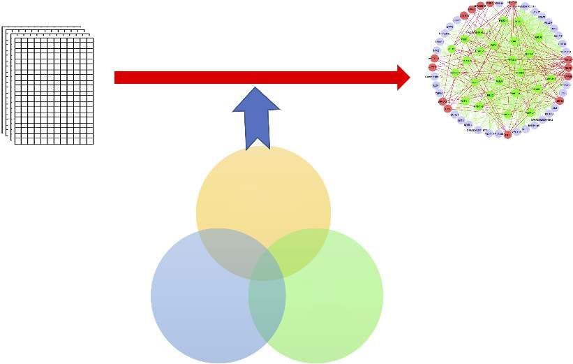
Huber-Berhu partial least squares regression
Therefore (13) can be solved iteratively by updating u and v grid of possible values. If the sample size is too small, CV can
alternately. Note, it is not cost-efficient to spend a lot of effort be replaced by leave-one-out validation; this procedure is
optimizing over u in line 6 before a good estimate for v is also used in for tuning penalization parameters[37,49].
computed. Since Algorithm 1 is an iterative algorithm, it may To choose the dimension of PLS, the Q2h criteria were
make sense to stop the optimization over u early before adopted. Q2h criteria were first proposed by Tenenhaus[50].
updating v . In the implementation, one step of proximal These criteria characterize the predictive power of the PLS
mapping was used to update u and v . That is: model by performing cross-validation computation. Q2h is
( ) defined as:
∂H (M − uv′ ) ∑q
u = Proxt,λB u − t (16) PRES S kh
∂u Q2h = 1− ∑
k=1
q k
( ) k=1 RS S h
∂H (M − uv′ )
v = Proxt,λB v − t (17) ∑n 2
∂v where PRES S kh = i=1 (yi − ŷh(−i) ) is the
k k Prediction Error Sum
∑ 2
The algorithm for finding the solution of the Huber–Berhu of Squares, and RS S kh = ni=1 (yki − ŷkh ) is the Residual Sum of
PLS regression in (13) is detailed in Algorithm 2. Squares for the variable k and the PLS dimension h. The criterion
for determining if ξh contributes significantly to the prediction is:
Algorithm 2: Finding the solution of the Huber-Berhu PLS regression ( )
Input: TF matrix (X ), pathway matrix (Y ), penalty constant (λ ), and Q2h ≥ 1 − 0.952 = 0.0975
number of components (K ) This criterion is also used in SIMCA-P software[51] and
Output: regression coefficient matrix (A) sparse PLS[38]. However, the choice of the PLS dimension still
1 X0 = X, X0 = Y , cF = I , A = 0
remains an open question. Empirically, there is little biological
2 For k in 1,...,K
meaning when h is large and good performance appears in
3 set M k−1 = X ′k−1 Y k−1 2−5 dimensions.
4 Initialize u to be the first left singular vector and initialize v to
be the product of first right singular vectors and first singular
value. RESULTS
5 until convergence of u and v
6 update u using (16) The efficiency of the proximal gradient descent
7 update v using (17) algorithm
8 extract component ξ = Xu
compute regression coefficients in (8) c = X ′ ξ/(ξ′ ξ), d = Y ′ ξ/ We developed the proximal gradient descent algorithm
9 ′
(ξ ξ) (Algorithm 1) to solve Huber-Berhu regression. As compared
10 update A = A + cF · u · d′ to CVX, it could reduce the running time to at least 10 times,
11 update cF = cF · (I − u · c′ ) but up to 90 times in a desktop computer with 2.2 GHz Intel
12 compute residuals for X and Y , X = X − ξc′ , Y = Y − ξd Core i7 processor and 16 GB 1600 MHz DDR3 memory for a
setting of m and p based on 30 replications. For different m,
Tuning criteria and choice of the PLS dimension the patterns are similar (Fig. 3). More details can be found in
The Huber-Berhu PLS regression has two tuning parameters, the Deng 2018[52].
namely, the penalization parameter λ and the number of Validation of Huber-Berhu PLS with lignin
hidden components K . To select the best penalization para- biosynthesis pathway genes and regulators
meter, λ , a common k -fold cross-validation (CV) procedure The HB-PLS algorithm was examined for its accuracy in
that minimizes the overall prediction error is applied using a identifying lignin pathway regulators using the A. thaliana
m = 40 m = 100 m = 200
50 CVX CVX CVX
Algorithm 1 60 Algorithm 1 Algorithm 1
80
40
50
60
30 40
Time/s
Time/s
Time/s
30 40
20
20
10 20
10
0 0 0
50 100 200 500 1 000 5 000 50 100 200 500 1 000 5 000 50 100 200 500 1 000 5 000
p p p
Fig. 3 Comparison of running time for Algorithm 1 and CVX. p is the number of independent variables in TF-matrix (X ).
Page 6 of 13 Deng et al. Forestry Research 2021, 1: 6
Huber-Berhu partial least squares regression

microarray compendium data set produced from stem                               Prediction of photosynthetic pathway regulators in
tissues[40]. TFs identified by HB-PLS were compared to those                    Arabidopsis thaliana using Huber-Berhu PLS
identified by SPLS. The 50 top TFs that were ranked based on                       Photosynthesis is mediated by the coordinated action of
their connectivities with the lignin biosynthesis pathway                       approximately 3,000 different proteins, commonly referred to
genes were identified using HB-PLS (Fig. 4a) and compared to                    as photosynthesis proteins[56]. In this study, we used genes
those identified by SPLS (Fig. 4b), respectively. The lignin                    from the photosynthesis light reaction pathway and Calvin
biosynthesis pathway genes are shown in Fig. 4c. The positive                   cycle pathway to study which regulatory genes can
lignin biosynthesis pathway regulators, which are supported                     potentially control photosynthesis. Analysis was performed
by literature evidence, are shown in coral color. The HB-PLS                    using HB-PLS, with SPLS as a comparative method. The
algorithm identified 15 known lignin pathway regulators. Of                     compendium data set we used is comprised of 238 RNA-seq
these, MYB63, SND3, MYB46, MYB85, LBD15, SND1, SND2,                            data sets from Arabidopsis thaliana leaves that were under
MYB103, MYB58, MYB43, NST2, GATA12, VND4, NST1, MYB52,                          normal/untreated conditions. Expression data for 1389 TFs
are positive known transcriptional activators of lignin                         and 130 pathway genes were extracted from the above
biosynthesis in the SND1-mediated transcriptional regulatory                    compendium data set and used for analyses. The results of
network[53], and LBD15[54] and GATA12[55] are also involved in                  HB-PLS and SPLS methods are shown in Fig. 5a and 5b,
regulating various aspects of secondary cell wall synthesis.                    respectively, where 33 rather than 50 TFs were shown
Interestingly, SPLS identified the same set of positive pathway                 because the SPLS method only identified 33 TFs. Of the top
regulators as HB-PLS though their ranking orders are different.                 33 candidate TFs in the lists, HB-PLS identified 11 positive

     a                                                                     b

    Phenylalanine                                                                                                                                 c
             PAL3
                      C4H                      C3H                    COMT                         F5H                       COMT
                                                                                                           5-hydroxy
    Cinnamic acid            p-coumaric acid           Caffeic acid               Ferulic acid             ferulic acid             Sinapic acid
                                       4CL                    4CL                         4CL                    4CL                     4CL
                HCT                                                                                                          COMT
                                                                                                         5-hydroxy
                             p-coumaroyl coA           Caffeoyl coA      Feruloyl coA                    feruloyl coA               Sinapoyl coA
                                                                  CCoAOMT
                                                                                  CCR                                                    CCR
                                                                                                   F5H                       COMT
                                 Caffeat         4CL                                                     5-hydroxy-
                                                                               Coniferaldehyde           coniferaldehyde            Sinapaldehyde
                                                              HCT                         CAD                                            CAD
                      C3H                                                                          F5H                       COMT
     p-coumaroyl                                                                                         5-hydroxy-                 Sinapyl
                                 Caffeoyl                                      Coniferyl alcohol         coniferyl alcohol
     shikimic acid                                                                                                                  alcohol
                               shikimic acid
                                                                                Guaiacyl ligni                                  Syringyl lignin

  Fig. 4     The implementation of Huber-Berhu-Partial Least Squares (HB-PLS) to identify candidate regulatory genes controlling lignin
  biosynthesis pathway. (a) HB-PLS; (b) SPLS. Green nodes (inside the circles) represent lignin biosynthesis genes. Coral nodes represent positive
  lignin pathway regulators supported by existing literature, and shallow purple nodes contain other predicted transcription factors that are not
  supported by current available literature. (c) The lignin biosynthesis pathway.

Deng et al. Forestry Research 2021, 1: 6                                                                                                  Page 7 of 13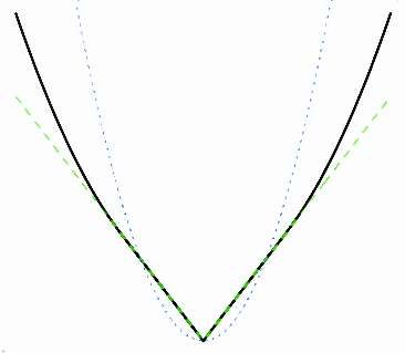
Huber-Berhu partial least squares regression

known TFs while SPLS identified 6 positive known TFs. IAA7,                   temperatures studied[71]. GATA phytochrome interacting
also known as AXR2, is regulated by HY5[57], which binds to G-                factor transcription factors regulate light-induced vindoline
box in LIGHT-HARVESTING CHLOROPHYLL A/B (Lhcb) pro-                           biosynthesis in Catharanthus roseus[72]. A number of genes
teins[58]. STO, also known as BBX24, whose protein physically                 show greater than 2-fold higher expression in light-grown
interacts with photosynthesis regulator HY5 to control photo-                 than dark-grown seedlings with the greatest differences
morphogenesis[59]; PHYTOCHROME-INTERACTING FACTOR                             observed for GATA6, GATA7, GATA21-23[68], with GATA6 and 7
(PIF) family have been shown to affect the expression of                      showing about 6- and 4-fold difference in expression levels.
photosynthesis-related genes, including genes encoding                        GATA11 is found to be a hub regulator of photosynthesis and
LHCA, LHCB, and PsaD proteins[60−62]. PIFs repress chloroplast                Chlorophyll biosynthesis[73]. The GLK transcription factors
development and photomorphogenesis[62]; PIF7, together                        promote the expression of many nuclear-encoded photo-
with PIF3 and PIF4, regulates responses to prolonged red                      synthetic genes that are associated with chlorophyll biosyn-
light by modulating phyB levels[63]. PIF7 is also involved in the             thesis and light-harvesting functions[74]; HSFA1, a master
regulation of circadian rhythms. GLK2, directly regulate the                  regulator of transcriptional regulation under heat stress,
expression of a series of photosynthetic genes including the                  regulates photosynthesis by inducing the expression of
genes encoding the PSI-LHCI complex and PSII-LHCII                            downstream transcription factors[75]. BEH1 is a homolog of
complex[64,65]. The plastid sigma-like transcription factor SIG1              BZR1, genetic analysis indicates that the BZR1-PIF4 interaction
regulate psaA respectively[66]; TOC1 is a member of the PRR                   controls a core transcription network by integrating
(PSEUDO-RESPONSE REGULATOR) family that includes PRR9,                        brassinosteroids and light response[76].
PRR7, PRR5, PRR3, and PRR1/TOC1. HY5 also binds and                           The performance and sensitivity of HB-PLS using
regulates the circadian clock gene PRR7, which affects the                    SPLS as a comparison
operating efficiency of PSII under blue light[67]. GATA trans-                   We tested the HB-PLS method in comparison with SPLS
cription factors have implicated some proteins in light-                      using two metabolic pathways, lignin biosynthesis pathway
mediated and circadian-regulated gene expression[68,69],                      and a unified photosynthesis pathway whose regulatory
GATAs can bind to XXIII box, a cis-acting elements involved in                genes are largely and partially known, respectively. We found
light-regulated expression of the nuclear gene GAPB, which                    that HB-PLS could identify more positive known TFs that are
encodes the B subunit of chloroplast glyceraldehyde-3-                        supported by existing literature in the output lists. To
phosphate dehydrogenase in A. thaliana[70]. In addition, GATA                 examine which methods can rank relatively more positive
interacts with SORLIP motifs in the 3-hydroxy-3-                              known TFs to the top of output regulatory gene lists, we
methylglutaryl-CoA reductase (HMGR) promoter of Picrorhiza                    plotted receiver operating characteristic curves (ROC) and
kurrooa, a herb plant, for the control of light-mediated                      calculated the area under the ROC curve (AuROC), which
expression; upstream sequences of HMGR of P. kurrooa                          reflects the sensitivity versus 1-specificity of a method. The
(PropkHMGR)-mediated gene expression was higher in the                        results are shown in Fig. 6. For lignin biosynthesis pathway,
dark as compared to that in the light in A. thaliana across four              HB-PLS was capable of ranking more positive known pathway

     a                                                                    b

  Fig. 5 The implementation of Huber-Berhu-Partial Least Squares (HB-PLS) to identify candidate regulatory genes (purple and coral nodes)
  controlling photosynthesis and related pathway genes. (a) was compared with the sparse partial least squares (SPLS) method (b) in identifying
  regulators that affects maize photosynthesis light reaction and Calvin cycle pathway genes. The green and yellow nodes within the cycles
  represent photosynthesis light reaction pathway genes and Calvin cycle pathway genes, respectively. Coral nodes in the circles represent
  positive predicted biological process or pathway regulators that are supported by existing literature, and shallow purple nodes contain other
  predicted TFs that do not have experimentally validated supporting evidence at present.

Page 8 of 13                                                                                            Deng et al. Forestry Research 2021, 1: 6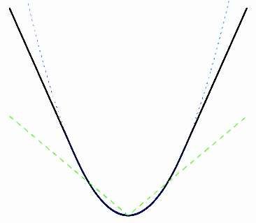
Huber-Berhu partial least squares regression

                 a                                                                           b
                                            1.0                                                                         1.0

                                            0.8                                                                         0.8
                 True positive rate (TPR)

                                                                                             True positive rate (TPR)
                                            0.6                                                                         0.6

                                            0.4                                                                         0.4

                                            0.2                                                                         0.2
                                                                 HB-PLS (AuROC = 0.94)                                                       HB-PLS (AuROC = 0.49)
                                                                 SPLS (AuROC = 0.73)                                                         SPLS (AuROC = 0.64)
                                             0                                                                           0
                                                  0   0.2      0.4      0.6      0.8   1.0                                    0   0.2      0.4       0.6     0.8   1.0
                                                        False positive rate (FPR)                                                    False positive rate (FPR)
  Fig. 6 The receiver operating characteristic (ROC) curves of Huber-Berhu-partial least squares (HB-PLS) and sparse partial least squares (SPLS)
  methods for identifying pathway regulators in Arabidopsis thaliana. (a) Lignin biosynthesis pathway; (b) a merged pathway of light reaction
  pathway and Calvin cycle pathway.

regulators to the top in the inferred regulatory gene list. As a                                          DISCUSSION
result, the AuROC of HB-PLS (0.94) (Fig. 6a) is much large than
that of SPLS (0.73) (Fig. 6b). For the unified light reaction and                                            The identification of gene regulatory relationships through
Calvin cycle pathway, the true pathway regulators have not                                                constructing GRNs from high-throughput expression data
been fully identified, and they are only partially known.                                                 sets has some inherent challenges due to high dimensionality
Although SPLS only identified the 6 positive known pathway                                                and multicollinearity. High dimensionality is caused by a
regulators in comparison with 10 identified by HB-PLS, SPLS                                               multitude of gene variables while multicollinearity largely
                                                                                                          results from a large number of genes versus a relatively small
ranked 4 out 6 positive known pathway regulators to the top
                                                                                                          sample size. In this study, we combined three types of
8 positions, resulting in slightly higher sensitivity versus 1-
                                                                                                          computational approaches, statistics (PLS), machine learning
specificity. HB-PLS identified 10 positive known regulators
                                                                                                          (Semi-unsupervised learning) and convex optimization
among the top 33 regulatory genes, which are more evenly
                                                                                                          (Berhu and Huber) for simulating gene regulatory relation-
distributed in the list, resulting in relatively smaller AuROC
                                                                                                          ships, as illustrated in Fig. 7, and our results showed this
(0.49) as compared to the AuROC of SPLS (0.64). The overall
                                                                                                          integrative approach is viable and efficient.
lower AuROC values for both methods for photosynthesis
                                                                                                             One method that we frequently use to deal with dimen-
pathway are probably owing to the low number of positive
                                                                                                          sionality and multicollinearity is partial least squares (PLS),
known regulatory genes for this pathway.
                                                                                                          which couples dimension reduction with a regression model.
   Given the fact that lignin biosynthesis pathway regulators
                                                                                                          However, because PLS is not particularly suited for
have been well identified and characterized experimentally[77],                                           variable/feature selection, it often produces linear combi-
they are specifically suited for examining the efficiency of the                                          nations of the original predictors that are hard to interpret
HB-PLS method for each pathway gene. We selected two                                                      due to high dimensionality[78]. To solve this problem, Chun
methods, SPLS and PLS, as comparisons. For each output TF                                                 and Keles developed an efficient implementation of sparse
list to a pathway gene yielded from one of three methods, we                                              PLS, referred to as the SPLS method, based on the least angle
applied a series of cutoffs, with the number of TFs retained                                              regression[79]. SPLS was then benchmarked by means of
varying from 1 to 40 in a shifting step of 1 at a time, and then                                          comparisons to well-known variable selection and dimension
counted the number of positive regulatory genes in each of                                                reduction approaches via simulation experiments[78]. We used
the retained lists. The results are shown in Supplementary                                                the SPLS method in our previous study[41] and found that it
Fig. S1. It is obvious that for almost every pathway gene, HB-                                            was highly efficient in identifying pathway regulators and
PLS has higher sensitivity versus specificity.                                                            thus used it as a benchmark for evaluating the new methods.
   The results indicate that the HB-PLS and SPLS regressions,                                                In this study, we developed a PLS regression that incorpo-
in many cases, are much more efficient in recognizing                                                     rates the Huber loss function and the Berhu penalty for
positive regulators to a pathway gene compared to the PLS                                                 identification of pathway regulators using high-throughput
regression (Supplementary Fig. S1). For most pathway genes                                                gene expression data (with dimensionality and multicolli-
like PAL1, C4H, CCR1, C3H, and COMT1, HB-PLS method could                                                 nearity). Although the Huber loss function and the Berhu
identify more positive regulators in the top 20 regulators as                                             penalty have been proposed in regularized regression
compared to the SPLS method. For HCT, CCoAOMT1, CAD8,                                                     models[43,80], this is the first time that both of them were
and F5H, HB-PLS was almost always more efficient than SPLS                                                combined with the PLS regression at the same time. The
when the top cut-off lists contained fewer than 40 regulators.                                            Huber function is a combination of linear and quadratic loss
For pathway gene CAD8, both SPLS and PLS both failed to                                                   functions. In comparison with other loss functions (e.g.,
identify positive regulators while HB-PLS performed more                                                  square loss and least absolute deviation loss), Huber loss is
efficiently.                                                                                              more robust to outliers and has higher statistical efficiency

Deng et al. Forestry Research 2021, 1: 6                                                                                                                                 Page 9 of 13
Huber-Berhu partial least squares regression
Samples
Modeling with machine learning, statistics and
convex optimization combined approaches
Genes
Biological process &
pathway network
Convex Alternative
optimization minimization
Machine Semi-Unsupervised
PLS method Statistics learning
learning
Fig. 7 An integrative framework for identifying biological process and pathway regulators from high-throughput gene expression data by
integration of statistics, machine learning and convex optimization. PLS: Partial least squares.
than the LAD loss function in the absence of outliers. The two pathways we analyzed, and the sensitivity of HB-PLS is
Berhu function[33] is a hybrid of the ℓ2 penalty and the ℓ1 much better than that of SPLS for lignin pathway whose
penalty. It gives a quadratic penalty to large coefficients and a regulatory genes are more complete, and slightly worse than
linear penalty to small coefficients. Therefore, the Berhu that of HB-PLS for photosynthesis light reaction and Calvin
penalty has advantages of both the ℓ2 and ℓ1 penalties: cycle pathway (Fig. 5 and Supplementary Fig. S1) whose
smaller coefficients tend to shrink to zero while the regulatory genes are only partially known. Therefore, HB-PLS
coefficients of a group of highly correlated predictive has an overall larger advantage. Unfortunately, except the
variables are not changed much if their coefficients are large. two pathways we evaluated, there are almost no other
A comparison of HB-PLS with SPLS and also PLS suggests metabolic pathways whose regulatory genes have been
that HB-PLS can identify more true pathway regulators. This is mostly identified. Our analysis showed that the two methods
an advantage over either SPLS or PLS (Supplementary Fig. S1) could empower the recognition of pathway regulators
when experimental validation is concerned. The application including some unique pathway regulators, and thus are
of HB-PLS and SPLS methods to identification of lignin useful in continued research.
biosynthesis pathway regulators in A. thalian led to the
identification of 15 and 15 positive pathway regulators, CONCLUSIONS
respectively, while application of the HB-PLS and SPLS
methods to identification of photosynthesis pathway A new method called the HB-PLS regression was developed
regulators in A. thalian resulted in 10 and 6 positive pathway for identifying biological process or pathway regulators by
regulators, respectively. The outperformance of HB-PLS over integration of statistics, machine learning and convex
SPLS (Fig. 6a) and PLS (Supplementary Fig. S1) implicates that optimization approaches. In HB-PLS, an accelerated proximal
the use of Huber loss function and Berhu penalty function for gradient descent algorithm was specifically developed to
convex optimization contributed to the recognition of true solve Huber and Berhu optimization, which can estimate the
pathway regulators and rank them at the top of the output regression parameters by optimizing the objective function
lists. It also suggests the viability and the increased power of based on the Huber and Berhu functions. Characteristic
combination of statistics (PLS), machine learning (Semi- analysis of the Huber-Berhu regression indicated it could
unsupervised learning) and convex optimization (Berhu and identify sparse solution. When modeling the gene regulatory
Huber) for recognition of regulatory relationships. In addition, relationships from regulatory genes to pathway genes, HB-
the ROC plotting suggests that HB-PLS method has PLS is capable of dealing with the high multicollinearity of
comparable sensitivity versus 1-specificity compared to SPLS both regulatory genes and pathway genes. Application of the
because HB-PLS achieved a higher AuROC for lignin HB-PLS to real A. thaliana high-throughput data showed that
biosynthesis pathway but a lower AuROC for the unified HB-PLS could identify majority positive known regulatory
photosynthesis pathway as compared to SPLS (Fig. 6). genes that govern two pathways. Sensitivity verse 1-
However, the fact that the HB-PLS identified the same or specificity plotting showed that HB-PLS could rank more
higher number of positive true regulators than SPLS for the positive known regulators to the top of output regulatory
Page 10 of 13 Deng et al. Forestry Research 2021, 1: 6Huber-Berhu partial least squares regression
gene lists for lignin biosynthesis pathways while SPLS can 8. Cao J, Qi X, Zhao H. 2012. Modeling gene regulation networks
rank more for the unified photosynthesis pathway. Our study using ordinary differential equations. In Next Generation
suggests that the overall performance of HB-PLS exceeds that Microarray Bioinformatics. Methods in Molecular Biology (Methods
of SPLS but both methods may have comparable and Protocols), eds. Wang J, Tan AC, Tian T, vol 802. USA:
Humana Press. pp: 185−97 https://doi.org/10.1007/978-1-61779-
sensitivity/specificity and are instrumental for identifying real
400-1_12
biological process and pathway regulators from high-
9. Sima C, Hua J, Jung S. 2009. Inference of Gene Regulatory
throughput gene expression data.
Networks Using Time-Series Data: A Survey. Current genomics
10:416−29
ACKNOWLEDGEMENTS 10. de la Fuente A, Bing N, Hoeschele I, Mendes P. 2004. Discovery of
meaningful associations in genomic data using partial
NSF Plant Genome Program [1703007 to SL and HW]; NSF correlation coefficients. Bioinformatics 20:3565−74
Advances in Biological Informatics [dbi-1458130 to HW]; 11. Schäfer J, Strimmer K. 2005. An empirical Bayes approach to
USDA McIntire-Stennis Fund to HW. inferring large-scale gene association networks. Bioinformatics
21:754−64
Availability of R Package: The R code and sample data for 12. Butte A, Kohane I. 2000. Mutual information relevance networks:
HB-PLS is available at github https://github.com/hwei0805/ Functional genomic clustering using pairwise entropy measure-
HB-PLS. For the R code of SPLS, please write to Dr. Wei ments. In Proceedings of Pacific Symposium on Biocomputing
(hairong@mtu.edu) to request. 2000, 5:704. USA: World Scientific. pp.415−26
https://doi.org/10.1142/4316
13. Margolin AA, Nemenman I, Basso K, Wiggins C, Stolovitzky G, et
Conflict of interest al. 2006. ARACNE: an algorithm for the reconstruction of gene
The authors declare that they have no conflict of interest. regulatory networks in a mammalian cellular context. BMC
Bioinformatics 7(Suppl 1):S7
14. Altay G, Emmert-Streib F. 2010. Inferring the conservative causal
Supplementary Information accompanies this paper at
core of gene regulatory networks. BMC Systems Biology 4:132
(http://www.maxapress.com/article/doi/10.48130/FR-2021-
15. Meyer PE, Lafitte F, Bontempi G. 2008. minet: A R/Bioconductor
0006) package for inferring large transcriptional networks using
mutual information. BMC Bioinformatics 9:461
Dates 16. Huynh-Thu VA, Geurts P. 2019. Unsupervised Gene Network
Inference with Decision Trees and Random Forests. In Gene
Received 11 March 2021; Accepted 11 March 2021; Regulatory Networks. Methods in Molecular Biology, eds.
Published online 30 March 2021 Sanguinetti G, Huynh-Thu VA, vol 1883. New York: Humana
Press. pp. 195−215 https://doi.org/10.1007/978-1-4939-8882-2_8
17. Deng W, Zhang K, Busov V, Wei H. 2017. Recursive random forest
REFERENCES algorithm for constructing multilayered hierarchical gene
1. Chen T, He HL, Church GM. 1999. Modeling gene expression with regulatory networks that govern biological pathways. PLoS One
differential equations. In Proceeding of the Pacific Symposium on 12:e0171532
Biocomputing 1999, 4:611. USA: World Scientific. pp.29−40 18. Butte AJ, Tamayo P, Slonim D, Golub TR, Kohane IS. 2000.
https://doi.org/10.1142/3925 Discovering functional relationships between RNA expression
2. Kauffman S. 1969. Homeostasis and differentiation in random and chemotherapeutic susceptibility using relevance networks.
genetic control networks. Nature 224:177−8 Proc. Natl. Acad. Sci. U. S. A. 97:12182−6
3. Chen BS, Chang CH, Wang YC, Wu CH, Lee HC. 2011. Robust 19. Faith JJ, Hayete B, Thaden JT, Mogno I, Wierzbowski J, et al. 2007.
model matching design methodology for a stochastic synthetic Large-scale mapping and validation of Escherichia coli
gene network. Math. Biosci. 230:23−36 transcriptional regulation from a compendium of expression
4. Friedman N, Nachman I, Pe'er D. 1999. Learning bayesian profiles. PLoS Biol. 5:e8
network structure from massive datasets: the "sparse candidate" 20. Meyer PE, Kontos K, Lafitte F, Bontempi G. 2007. Information-
algorithm. Proceedings of the Fifteenth Conference on Uncertainty
theoretic inference of large transcriptional regulatory networks.
in Artificial Intelligence (UAI1999). pp. 206−15. Stockholm:
EURASIP journal on bioinformatics and systems biology
Morgan Kaufmann Publishers Inc.
2007:79879 https://rdcu.be/chDK7
5. Friedman N, Linial M, Nachman I, Pe'er D. 2000. Using Bayesian
networks to analyze expression data. Journal of Computational 21. Gunasekara C, Zhang K, Deng W, Brown L, Wei H. 2018. TGMI: an
Biology 7:601−20 efficient algorithm for identifying pathway regulators through
6. Chai LE, Law CK, Mohamad MS, Chong CK, Choon YW, et al. 2014. evaluation of triple-gene mutual interaction. Nucleic Acids Res.
Investigating the effects of imputation methods for modelling 46:e67
gene networks using a dynamic bayesian network from gene 22. Zhang X, Zhao X, He K, Lu L, Cao Y, et al. 2012. Inferring gene
expression data. Malays J Med Sci 21:20−7 https://pubmed.ncbi. regulatory networks from gene expression data by path
nlm.nih.gov/24876803/ consistency algorithm based on conditional mutual information.
7. Exarchos TP, Rigas G, Goletsis Y, Stefanou K, Jacobs S, et al. 2014. Bioinformatics 28:98−104
A dynamic Bayesian network approach for time-specific survival 23. Meinshausen N, Bühlmann P. 2006. High-dimensional graphs
probability prediction in patients after ventricular assist device and variable selection with the Lasso. Annals of statistics
implantation. 2014 36th Annual International Conference of the 34:1436−62
IEEE Engineering in Medicine and Biology Society, Chicago, IL, USA, 24. Zhang X, Liu K, Liu Z, Duval B, Richer JM, et al. 2013. NARROMI: a
2014, pp. 3172−5. USA: IEEE https://doi.org/doi:10.1109/EMBC. noise and redundancy reduction technique improves accuracy
2014.6944296 of gene regulatory network inference. Bioinformatics 29:106−13
Deng et al. Forestry Research 2021, 1: 6 Page 11 of 13Huber-Berhu partial least squares regression
25. Hayes AF, Cai L. 2007. Using heteroskedasticity-consistent 46. Yu YL. 2013. On decomposing the proximal map. NIPS'13:
standard error estimators in OLS regression: an introduction and Proceedings of the 26th International Conference on Neural
software implementation. Behav. Res. Methods 39:709−22 Information Processing Systems, Lake Tahoe, Nevada, 2013, vol
26. Hoerl AE, Kennard RW. 1970. Ridge regression: Biased estimation 1:91−9. New York: Curran Associates Inc. https://proceedings.
for nonorthogonal problems. Technometrics 12:55−67 neurips.cc/paper/2013/file/98dce83da57b0395e163467c9dae52
27. Tibshirani R. 1996. Regression shrinkage and selection via the 1b-Paper.pdf
lasso. Journal of the Royal Statistical Society: Series B 47. Beck, A. and M. Teboulle. 2009. A fast iterative shrinkage-
(Methodological) 58:267−88 thresholding algorithm for linear inverse problems. SIAM journal
28. Zou H. 2006. The adaptive lasso and its oracle properties. J. Am. on imaging sciences 2(1):183−202
Stat. Assoc. 101:1418−29 48. Vinzi VE, Russolillo G. 2013. Partial least squares algorithms and
29. Zou H, Hastie T. 2005. Regularization and variable selection via methods. WIREs Computational Statistics 5:1−19
the elastic net. Journal of the Royal Statistical Society: Series B 49. Shen H, Huang JZ. 2008. Sparse principal component analysis via
(Statistical Methodology) 67:301−20 regularized low rank matrix approximation. Journal of
30. Wang H, Li G, Jiang G. 2007. Robust regression shrinkage and multivariate analysis 99:1015−34
consistent variable selection through the LAD-Lasso. Journal of 50. Tenenhaus A, Guillemot V, Gidrol X, Frouin V. 2010. Gene
Business & Economic Statistics 25:347−55 association networks from microarray data using a regularized
31. Yu C, Yao W. 2017. Robust linear regression: A review and estimation of partial correlation based on PLS regression.
comparison. Communications in Statistics - Simulation and IEEE/ACM Trans Comput Biol Bioinform 7:251−62
Computation 46:6261−82 51. Simca P. 2002. SIMCA-P+ 10 Manual. Umetrics AB
32. Lambert-Lacroix S, Zwald L. 2011. Robust regression through the 52. Deng W. 2018. Algorithms for reconstruction of gene regulatory
Huber’s criterion and adaptive lasso penalty. Electronic Journal of networks from high -throughput gene expression data. PhD. Open
Statistics 5:1015−53 Access Dissertation. Michigan Technological University. pp. 101
33. Owen AB. 2007. A robust hybrid of lasso and ridge regression. https://digitalcommons.mtu.edu/etdr/722/
Proceedings of the AMS-IMS-SIAM Joint Summer Research 53. Zhou J, Lee C, Zhong R, Ye ZH. 2009. MYB58 and MYB63 are
Conference on Machine and Statistical Learning: Prediction and transcriptional activators of the lignin biosynthetic pathway
Discovery, Snowbird, UT, 2006, Contemporary Mathematics during secondary cell wall formation in Arabidopsis. Plant Cell
443:59−72. Providence, RI: American Mathematical Society 21:248−66
http://www.ams.org/books/conm/443/ 54. Shuai B, Reynaga-Peña CG, Springer PS. 2002. The lateral organ
34. Zwald L, Lambert-Lacroix S. 2012. The BerHu penalty and the boundaries gene defines a novel, plant-specific gene family.
grouped effect. arXiv preprint arXiv: 1207.6868 Plant Physiol. 129:747−61
35. Grant M, Boyd S, Ye Y. 2008. CVX: Matlab software for disciplined 55. Nishitani K, Demura T. 2015. Editorial: An Emerging View of Plant
convex programming. http://cvxr.com/cvx/ Cell Walls as an Apoplastic Intelligent System. Plant and Cell
36. Sæbø S, Almøy T, Aarøe J, Aastveit AH. 2007. ST-PLS: a multi- Physiology 56:177−9
directional nearest shrunken centroid type classifier via PLS. 56. Wang P, Hendron RW, Kelly S. 2017. Transcriptional control of
Chemometrics 22:54−62 photosynthetic capacity: conservation and divergence from
37. Chun H, Keleş S. 2010. Sparse partial least squares regression for Arabidopsis to rice. New Phytol. 216:32−45
simultaneous dimension reduction and variable selection. 57. Cluis CP, Mouchel CF, Hardtke CS. 2004. The Arabidopsis
Journal of the Royal Statistical Society: Series B (Statistical transcription factor HY5 integrates light and hormone signaling
Methodology) 72:3−25 pathways. Plant J. 38:332−47
38. Lê Cao K-A, Rossouw D, Robert-Granié C, Besse P. 2008. A sparse 58. Andronis C, Barak S, Knowles SM, Sugano S, Tobin EM. 2008. The
PLS for variable selection when integrating omics data. Statistical clock protein CCA1 and the bZIP transcription factor HY5
applications in genetics and molecular biology 7:Ariticl 35 physically interact to regulate gene expression in Arabidopsis.
39. Chaffey N, Cholewa E, Regan S, Sundberg B. 2002. Secondary Mol. Plant 1:58−67
xylem development in Arabidopsis: a model for wood formation. 59. Job N, Yadukrishnan P, Bursch K, Datta S, Johansson H. 2018.
Physiologia plantarum 114:594−600 Two B-Box Proteins Regulate Photomorphogenesis by
40. Kumari S, Deng W, Gunasekara C, Chiang V, Chen HS, et al. 2016. Oppositely Modulating HY5 through their Diverse C-Terminal
Bottom-up GGM algorithm for constructing multilayered Domains. Plant Physiol. 176:2963−76
hierarchical gene regulatory networks that govern biological 60. Jiang Y, Yang C, Huang S, Xie F, Xu Y, et al. 2019. The ELF3-PIF7
pathways or processes. BMC Bioinformatics 17:132 Interaction Mediates the Circadian Gating of the Shade
41. Zheng J, He C, Qin Y, Lin G, Park WD, et al. 2019. Co-expression Response in Arabidopsis. iScience 22:288−98
analysis aids in the identification of genes in the cuticular wax 61. Kim K, Jeong J, Kim J, Lee N, Kim ME, et al. 2016. PIF1 Regulates
pathway in maize. Plant J. 97:530−42 Plastid Development by Repressing Photosynthetic Genes in the
42. Trapnell C, Williams BA, Pertea G, Mortazavi A, Kwan G, et al. Endodermis. Molecular plant 9:1415−27
2010. Transcript assembly and quantification by RNA-Seq reveals 62. Shin J, Kim K, Kang H, Zulfugarov IS, Bae G, et al. 2009.
unannotated transcripts and isoform switching during cell Phytochromes promote seedling light responses by inhibiting
differentiation. Nat. Biotechnol. 28:511−5 four negatively-acting phytochrome-interacting factors. Proc.
43. Huber PJ. 2011. Robust statistics. In International Encyclopedia of Natl. Acad. Sci. U. S. A. 106:7660−5
Statistical Science, ed. Lovric M. Berlin, Heidelberg: Springer. pp. 63. Leivar P, Monte E, Al-Sady B, Carle C, Storer A, et al. 2008. The
1248−51 https://doi.org/10.1007/978-3-642-04898-2_594 Arabidopsis phytochrome-interacting factor PIF7, together with
44. Yi C, Huang J. 2017. Semismooth newton coordinate descent PIF3 and PIF4, regulates responses to prolonged red light by
algorithm for elastic-net penalized huber loss regression and modulating phyB levels. Plant Cell 20:337−52
quantile regression. Journal of Computational and Graphical 64. Waters MT, Wang P, Korkaric M, Capper RG, Saunders NJ,
Statistics 26:547−57 Langdale JA. 2009. GLK transcription factors coordinate
45. Parikh N, Boyd S. 2014. Proximal algorithms. Foundations and expression of the photosynthetic apparatus in Arabidopsis. The
Trends® in Optimization 1:127−239 Plant cell 21:1109−28
Page 12 of 13 Deng et al. Forestry Research 2021, 1: 6You can also read