High-resolution Transmission Spectroscopy of MASCARA-2 b with EXPRES
←
→
Page content transcription
If your browser does not render page correctly, please read the page content below
Astronomy & Astrophysics manuscript no. main_arxiv                                                                     c ESO 2020
                                               April 21, 2020

                                                High-resolution Transmission Spectroscopy of MASCARA-2 b
                                                                       with EXPRES
                                                 H. Jens Hoeijmakers1, 2 , Samuel H. C. Cabot3 , Lily Zhao3 , Lars A. Buchhave4 , René Tronsgaard4 , Daniel
                                                 Kitzmann2 , Simon L. Grimm2 , Heather M. Cegla1 , Vincent Bourrier1 , David Ehrenreich1 , Kevin Heng2, 5 ,
                                                                                 Christophe Lovis1 , and Debra A. Fischer3

                                                    1
                                                        Observatoire de Genève, Chemin des Maillettes 51, 1290, Versoix, Switzerland
                                                    2
                                                        Center for Space and Habitability, Universität Bern, Gesellschaftsstrasse 6, 3012 Bern, Switzerland
                                                    3
                                                        Yale University, 52 Hillhouse, New Haven, CT 06511, USA
                                                    4
                                                        DTU Space, National Space Institute, Technical University of Denmark, Elektrovej 328, DK-2800 Kgs. Lyngby,
arXiv:2004.08415v1 [astro-ph.EP] 17 Apr 2020

                                                        Denmark
                                                    5
                                                        University of Warwick, Department of Physics, Astronomy & Astrophysics Group, Coventry CV4 7AL, United
                                                        Kingdom

                                                    Received January 2, 2020; accepted April 17, 2020

                                                                                                          ABSTRACT

                                                    We report detections of atomic species in the atmosphere of MASCARA-2 b, using the first transit observations obtained
                                                    with the newly commissioned EXPRES spectrograph. EXPRES is a highly stabilised optical echelle spectrograph,
                                                    designed to detect stellar reflex motions with amplitudes down to 30 cm/s, and was recently deployed at the Lowell
                                                    Discovery Telescope. By analysing the transmission spectrum of the ultra-hot Jupiter MASCARA-2 b using the cross-
                                                    correlation method, we confirm previous detections of Fe i, Fe ii and Na i, which likely originate in the upper regions of
                                                    the inflated atmosphere. In addition, we report significant detections of Mg i and Cr ii. The absorption strengths change
                                                    slightly with time, possibly indicating different temperatures and chemistry in the day-side and night-side terminators.
                                                    Using the effective stellar line-shape variation induced by the transiting planet, we constrain the projected spin-orbit
                                                    misalignment of the system to 1.6 ± 3.1 degrees, consistent with an aligned orbit. We demonstrate that EXPRES joins
                                                    a suite of instruments capable of phase-resolved spectroscopy of exoplanet atmospheres.
                                               1. Introduction                                                    son et al. 2016) at the Isaac Newton Telescope are currently
                                                                                                                  under development.
                                               The emergence of a new generation of spectrographs opens               The EXtreme PREcision Spectrograph (EXPRES) was
                                               avenues for detecting and characterizing exoplanets and            commissioned at the Lowell Observatory 4.3-m Lowell Dis-
                                               their atmospheres with unprecedented fidelity. Exoplanets          covery Telescope (LDT, Levine et al. 2012) in 2018. EX-
                                               can be detected with high-resolution spectrographs due to          PRES is a vacuum-stabilized, fiber-fed, R ∼ 140, 000, opti-
                                               their gravitational interaction with the host-star, causing a      cal spectrograph with wavelength calibration from a Menlo
                                               periodic Doppler shift in the observed stellar spectrum as         Systems laser frequency comb (LFC). It is optimized for
                                               the planet orbits. These measurements yield a lower limit          wavelengths between 380 and 680 nm. The design goal of
                                               to the mass of the planet or the mass itself if the planet         EXPRES was a RV precision of ∼ 30 cm s−1 on bright (V <
                                               orbits in an aligned plane that carries it through transit         8) main sequence stars. Observations with the LFC demon-
                                               as seen from Earth. One may constrain the composition              strate an instrumental stability of 7 cm s−1 and formal er-
                                               of a transiting planet by also measuring its radius, which         rors of about 25 cm s−1 for an SNR of 250 when observing
                                               then yields the mean density. Recent years have seen exten-        bright stars (Blackman et al. 2019; Petersburg et al. 2020).
                                               sive efforts to develop a new generation of environmentally-           High resolution spectrographs are able to directly probe
                                               controlled high-resolution spectrographs that provide ever         spectral features in the atmospheres of exoplanets (Snellen
                                               increasing radial velocity (RV) precision and stability, to        et al. 2008). The high spectral resolution allows for individ-
                                               allow for more precise mass measurements, and for the de-          ual spectral lines in the planet’s spectrum to be resolved
                                               tection of less massive planets further away from their host       and provides measurements of the line-shape and depth
                                               star. Indeed, several purpose-built instruments have come          (e.g. Redfield et al. 2008; Wyttenbach et al. 2015; Jensen
                                               online in recent years. ESPRESSO (Pepe et al. 2013) was            et al. 2012; Khalafinejad et al. 2017; Wyttenbach et al. 2017;
                                               commissioned at the Very Large Telescope (VLT) in De-              Allart et al. 2019; Seidel et al. 2019). The orbital velocity of
                                               cember 2017. HARPS-N/GIANO (Cosentino et al. 2012;                 hot-Jupiters is often in excess of 100 km s−1 . At R ∼ 105 ,
                                               Claudi et al. 2017; Oliva et al. 2018) at Telescopio Nazionale     this motion is resolved in time-series exposures of a several-
                                               Galileo, CARMENES (Quirrenbach et al. 2010) at Calar               hour transit. Separating the spectrum of the planet from the
                                               Alto Observatory and SPIRou (Thibault et al. 2012) at the          host star using this Doppler shift was first applied to detect
                                               Canada France Hawaii Telescope provide high-resolution             absorption by atmospheric CO in the infra-red transmission
                                               optical and NIR coverage. NIRPS (Wildi et al. 2017) at the         spectrum of HD 209458 b (Snellen et al. 2010). Later efforts
                                               ESO’s 3.6-m telescope at La Silla and HARPS3 (Thomp-               employed this technique to detect the thermal emission of
                                                                                                                                                      Article number, page 1 of 20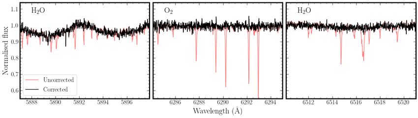
A&A proofs: manuscript no. main_arxiv

both transiting and non-transiting hot-Jupiters, resulting      for Mg i, Na i and Cr ii. We summarize our results in Section
in detections of CO, H2 O, CH4 and HCN (e.g. Brogi et al.       4.
2012; Birkby et al. 2013; Lockwood et al. 2014; Brogi et al.
2016; Piskorz et al. 2016; Birkby et al. 2017; Hawker et al.
2018; Cabot et al. 2019; Guilluy et al. 2019; Flagg et al.      2. Transit observations of MASCARA-2 b
2019). The technique has also been applied at optical wave-
lengths to detect TiO in the day-side spectrum of WASP-33       A single transit of M2 was observed with the LDT during
b using the HDS/Subaru instrument (Nugroho et al. 2017),        the night of June 1, 2018. The night was clear with an av-
and atomic metal lines in the transmission spectrum of          erage seeing of approximately 1."2. The observations lasted
KELT-9 b (Hoeijmakers et al. 2018a, 2019) using HARPS-          from 09:03 to 14:23 UTC, with a total of 68 exposures of
N/T N G and PEPSI/LBT (Cauley et al. 2019). Ongoing             the system, of which 51 were obtained in-transit (we include
improvements in resolution, stability, and wavelength cal-      ingress/egress in our in-transit sample). The signal to noise
ibration will enable more detailed detections of chemistry      ratio for these exposures reached approximately 40-50 near
and atmospheric dynamics for a multitude of exoplanet sys-      5000 Åthroughout the night. Most exposures were approxi-
tems (Heng & Showman 2015; Crossfield 2015; Madhusud-           mately 200 seconds, while 15-minute exposures at the start
han et al. 2016; Birkby 2018; Triaud 2018; Wright 2018).        of the night provided high S/N out-of-transit spectra.
As such, stabilized, fiber-fed high-resolution spectrographs        Wavelength calibration is carried out with a Menlo Sys-
have a complementary dual-use in the discovery of exoplan-      tems Laser Frequency Comb as well as a ThAr line-lamp.
ets as well as the characterization of their atmospheres.       Exposures are taken through the science fiber and are in-
    MASCARA-2 b/Kelt-20 b (hereafter M2) was inde-              terspersed with science observations approximately every
pendently discovered by the Multi-site All-Sky CAmeRA           30 minutes. A tune-able LED is used to take flat-fields.
(MASCARA) (Talens et al. 2018) and the Kilo-degree Ex-          Sets of zero-second bias frames are taken before and after
tremely Little Telescope (KELT) (Lund et al. 2017), which       the observing night, and dark current is corrected using
both survey bright stars for signs of periodically transit-     the CCD overscan regions. We perform extractions with
ing exoplanets. The planet is a hot-Jupiter, transiting the     the RePack1 code, adapted from a version purposed for use
bright (mV = 7.6) A2 main sequence star HD 185603 in a          with HARPS-N data products (Fischer et al. 2016). We
3.47 day orbit. The orbit of the planet is aligned, which       also divide spectra by a blaze-function derived from flat-
is not common for this type of star (Winn et al. 2010;          field calibrations. The result is a pipeline-reduced spectral
Schlaufman 2010; Albrecht et al. 2012). Strong irradiation      time series in Earth’s rest-frame, shown in the top panel of
from its host star gives M2 b a high equilibrium temper-        Figure 1.
ature of Teq ∼ 2260 K, placing it in the extreme class of           Our subsequent analysis follows the approach of Hoei-
ultra-hot Jupiters. Several such planets have been studied      jmakers et al. (2019) that resulted in the detections of
to date, most notably KELT-9 b, which, with Teq = 4050 K        iron and titanium in the atmosphere of KELT-9 b, using
is the hottest known planet around a main-sequence star.        a similar sequence of observations by the HARPS-N spec-
In light of previous detections of atomic metals in KELT-       trograph. The cross-correlation procedure discussed below
9 b (Hoeijmakers et al. 2018a, 2019), atmospheric studies       differs from the approach used by Casasayas-Barris et al.
of other ultra-hot Juptiers warrant searches for vaporized      (2018, 2019), which was based on the direct analysis of in-
metals and ions.                                                dividual absorption lines in a single, co-added transmission
    The transmission spectrum of M2 has been observed           spectrum.
extensively with the HARPS-N and CARMENES spectro-
graphs, leading to detections of two Balmer lines of hy-        2.1. Telluric Correction and Detrending
drogen, the Na i D-lines, the Ca ii infra-red triplet, Fe i,
Fe ii and tentative evidence for an Mg i line at 517.268        Absorption lines from the stellar photosphere as well as the
(Casasayas-Barris et al. 2018, 2019; Nugroho et al. 2020;       Earth’s atmosphere (telluric lines) are the most dominant
Stangret et al. 2020). These detections are indicative of the   spectral features in the observed spectra. We model the
high temperatures prevalent at the day-side and termina-        telluric contamination in each spectrum with the Molecfit
tor regions. The detection of strong hydrogen absorption        package (Smette et al. 2015). Molecfit processes an ob-
may further be indicative of an extended or evaporating         served spectrum along with ambient weather, time, and lo-
atmosphere (Yan & Henning 2018; Turner et al. 2020).            cation information to model the structure of the Earth’s
    This paper presents the results of one night of transit     atmosphere during an observation and to fit a line-by-line
observations of M2 with the EXPRES instrument, which            radiative transfer model to the spectrum. We use similar
constitute the first application of EXPRES for the purpose      initial parameters to those used by Allart et al. (2017), such
of exoplanet transit transmission spectroscopy. With these      as the atmospheric profile, degree of the continuum and
observations, we aim to demonstrate that EXPRES offers          wavelength polynomial fits, and resolution fit kernel. We
significant potential for atmospheric characterization in ad-   chose more relaxed convergence tolerances of 10−5 , which
dition to its main purpose of RV monitoring for exoplanet       improved runtime and the quality of fit. Because M2 is a
discovery. The paper is organized as follows: in section 2 we   fast rotator, most stellar lines are significantly broadened
describe the observations and present our analysis of the       and blended to form a quasi-continuum, minimizing their
transmission spectra. In section 3, we discuss our results,     effect on the fit of individual telluric lines. We fit each spec-
including analysis of the Doppler shadow induced by the         trum in the time-series individually and divide the spec-
Rossiter-McLaughlin effect. We detect spectroscopic signa-      trum by the fit to remove tellurics (Figure 1, middle and
tures of the atmosphere of M2 by confirming the presence of     bottom panels).
Fe i and Fe ii (Casasayas-Barris et al. 2019; Nugroho et al.
                                                                1
2020; Stangret et al. 2020), and presenting strong evidence         Written by Lars Buchhave

Article number, page 2 of 20
H. Jens Hoeijmakers et al.: EXPRES Transmission Spectroscopy of MASCARA-2 b
Fig. 1. Spectra obtained on June 1, 2018 with EXPRES. Top Panel: Time-series, high-resolution spectra cleaned and corrected
for tellurics. The orders are stitched together for visualization, but are analyzed independently during cross-correlation. Common
features such as stellar lines appear as dark columns. Inlet: Zoom-in of the time-series spectra between 5850-6000 Å (marked by
the green band), revealing the broadened Na doublet. Middle Panel: Example 1-dimensional spectrum from the time-series, before
(red) and after (black) telluric correction. The features around 6700 Å are an artifact of order stitching. Some strong stellar lines,
including the Balmer series and the Sodium D lines are marked. Bottom Panels: Zoom-in of the example 1-dimensional spectrum,
demonstrating the effect telluric correction in strongly contaminated regions (due to H2 O, O2 and H2 O, from left to right).
Our analysis uses spectra in the wavelength range 4000- 2013; Price-Whelan et al. 2018). The BERV changes by . 1
6800 Å. Bluer wavelengths are subject to very low in- km s−1 over the course of the transit. We do not correct
strumental throughput, and redder wavelengths suffer se- for stellar reflex motion. This effect is negligible because
vere telluric contamination that is more difficult to model M2 has broad absorption lines due to its fast rotation. We
while covering comparatively few atomic metal lines. This note the presence of excess absorption in the cores of the
leaves 64 out of 88 orders, which are treated separately un- Na doublet which we attribute to stationary ISM absorp-
til combining their individual cross-correlation functions at tion, as seen in previous analyses of M2 (Casasayas-Barris
the end of the analysis. For computational reasons, we re- et al. 2018, 2019). As in these studies, neglecting the stellar
sample all of the spectra onto a common wavelength grid reflex correction helps ensure the excess absorption cancels
of 0.01 Å spacing. We identify bad pixels (e.g. due to cos- during division by the master out-of-transit spectrum (see
mic ray hits) by selecting 5σ outliers in a sliding 500 pixel below). The 2.5% of pixels on either end of each order are
window, and setting them to the mean of the values in the masked from cross-correlation. This step removes edge arti-
window. We shift each spectrum into the rest-frame of the facts from shifting to the stellar rest-frame, as well as pixels
star, taking into account the -21.07 km s−1 systemic veloc- with low flux located at the edges of the blaze function.
ity (denoted Vsys ) (Talens et al. 2018) and the Barycentric We co-add all out-of-transit spectra {ft }t∈tout to ob-
Earth Radial Velocity (BERV) correction (calculated us- tain a master spectrum of the star Fout . We subsequently
ing the Astropy package, see Astropy Collaboration et al. compute individual transmission spectra {e rt }t∈tin by divid-
Article number, page 3 of 20A&A proofs: manuscript no. main_arxiv
ing each in-transit spectrum {ft }t∈tin by Fout (Wyttenbach (Collier Cameron et al. 2010; Bourrier et al. 2015), ignor-
et al. 2015; Allart et al. 2017; Hoeijmakers et al. 2018a; ing differential rotation of the stellar surface and convective
Casasayas-Barris et al. 2018, 2019). Finally, we apply a blueshift (Cegla et al. 2016):
high-pass Gaussian filter with 75 pixel standard-deviation
and subtract from the pixels in each wavelength bin their
time-average, removing broad-band variations (Hoeijmak- v∗ (t) = x⊥ (t)veq sin i∗ (1)
ers et al. 2018b).
where veq sin i∗ is the projected equatorial rotation ve-
locity of the star, and x⊥ is the orthogonal distance of the
2.2. Cross-correlation obscured region to the projected spin axis:
Atomic or molecular species present in the exoplanet at-
mosphere may cause thousands of individual absorption x⊥ (t) = xp (t) cos(λ) − yp (t) sin(λ) (2)
lines in the atmospheric transmission spectrum. Cross-
correlating the spectra with a model template spectrum where λ is the spin-orbit misalignment and xp (t) and
combines the contributions of all these lines to reduce the yp (t) are the coordinates of the planet:
photon-noise and yield significant detections of these ele-
ments (Snellen et al. 2010). We use high-resolution model a
spectra for Na i, Mg i, Sc i, Sc ii, Ti i, Ti ii, Cr i, Cr ii, Fe i, xp (t) = sin(2πφ) (3)
Fe ii and Y ii using opacities computed with HELIOS-K R∗
(Grimm & Heng 2015) and equilibrium chemistry at T =
4, 000 K with FastChem (Stock et al. 2018). These templates a
resulted in detections in the analysis of the transmission yp (t) = − cos(2πφ) cos(ip ) (4)
R∗
spectrum of KELT-9 b by Hoeijmakers et al. (2019), who
provide a detailed description of their construction. These with a the semi-major axis, R∗ the radius of the star,
templates are publicly accessible via the CDS 2 . ip the orbital inclination, φ the orbital phase at time t and
To compute the cross-correlation, we apply Doppler the orbital inclination ip .
shifts of -500 to 500 km s−1 to the template in increments The Doppler shadow is retrieved by cross-correlating the
of 1.0 km s−1 . At each velocity v, and for a given transmis- transmission spectra {e rt }t∈tin with a model template of the
sion spectrum ret , we take the weighted average of values in stellar spectrum. This template consists of a PHOENIX
the spectrum. The weights are a product of the Doppler- photosphere model spectrum at a temperature of 9000 K
shifted template, which is zero everywhere except at loca- and solar metallicity, obtained from the online PHOENIX
tions of line transitions, and the inverse of each wavelength library (Husser et al. 2013). The baseline of the template is
bin’s time-variance, which reduces the contribution of noisy subtracted via a high-pass filter so that it contains only the
pixels (Brogi et al. 2016). This procedure yields a cross- absorption lines with relative depths corresponding to the
correlation function (CCF) as a function of velocity and relative absorption of continuum radiation at each wave-
time, which contains the average line-strength of features length (i.e. continuum normalization).
in the transmission spectrum (Hoeijmakers et al. 2019). The resulting two-dimensional CCF contains the signa-
ture of the Doppler shadow (see the top panel in Figure 2),
from which the misalignment λ between the orbital plane
2.3. Rossiter-McLaughlin effect of the planet and the projected stellar spin axis can be de-
The orbit of M2 b is aligned (Lund et al. 2017; Talens et al. rived as is done when applying Doppler tomography (Collier
2018), meaning that the planet obscures the blue-shifted Cameron et al. 2010) or the “Reloaded RM-effect“ (Cegla
part of the star at the start of the transit, and moves to the et al. 2016). The shadow also overlaps with the expected
red-shifted part towards egress. This passage across the stel- RV of the planet, so it needs to be corrected before the sig-
lar disk changes the shapes of the disk-integrated, rotation- nature of the planet atmosphere may be isolated (see the
broadened stellar absorption lines, which gives rise to the second panel, "RM RV Model", in Figure 2; the local ob-
Rossiter-McLaughlin (RM) effect seen in the RV measure- structed RV overlaps the planetary RV, given by dashed and
ments of the star during transit (Ohta et al. 2005). For a dotted lines respectively). We construct a model of the two-
fast rotator like M2, broadened spectral features decrease dimensional cross-correlation residual from the parameters
the precision of RV measurements, making the RM effect of the Gaussian fits used to measure λ, following the ap-
difficult to resolve. However, when dividing the mean out- proach by Hoeijmakers et al. (2018a). This model is scaled
of-transit spectrum from each of the exposures, the line- to minimize the sum of the squared residual when subtract-
deformation causes the stellar lines to be over-corrected at ing it from cross-correlation functions with other the tem-
the instantaneous velocity of the obscured part of the stel- plates used in this analysis (see third and fourth panels,
lar disk. This effect is known as the "Doppler shadow" that "Shadow Model" and "Residual", in Figure 2). The Doppler
is cast by the planet as it progresses through transit (Col- shadow shows small variations in strength throughout the
lier Cameron et al. 2010). The centroid velocity v∗ (t) of the transit; darker regions are roughly correlated with higher
obscured stellar surface depends on the projected location exposure S/N. However, our empirical model is agnostic to
of the planet with respect to the stellar spin axis, which the origin of these variations, and successfully removes the
changes over time as the planet progresses through tran- shadow to isolate the atmospheric absorption. The overlap
sit, and is described by the following analytical expressions region between the atmospheric absorption trail and the
Doppler shadow may affect the co-added absorption signal;
2 however, as described by Hoeijmakers et al. (2018a), the
https://cdsarc.unistra.fr/viz-bin/cat?J/A+A/627/
A165 fit of Doppler shadow model ignores the overlap region and
Article number, page 4 of 20H. Jens Hoeijmakers et al.: EXPRES Transmission Spectroscopy of MASCARA-2 b
enforces smoothly varying model parameters, which helps where v̂∗ (t) is the model-predicted value of v∗ (t). We sub-
to preserve information at velocities for which the Doppler sequently perform a Markov Chain Monte Carlo (MCMC)
shadow and the planet absorption features overlap. This is analysis of the Doppler shadow to constrain orbital param-
possible because range of radial velocities spanned by the eters of the system.
Doppler shadow differs significantly different from those of We assume Gaussian priors on each of the orbital pa-
the planet atmosphere, due to the fast rotation of the host rameters, with mean and standard deviation as reported
star. by Talens et al. (2018) (see Table A.1). Our model con-
tains 5 parameters: scaled semi-major axis a/R∗ , projected
2.4. The time-averaged CCF obliquity λ, orbital inclination ip , projected stellar rotation
speed v sin i∗ , and a systematic RV offset to account for
The planet’s apparent RV is described by: errors in the systemic velocity. We place a Gaussian prior
on the offset with mean and standard deviation of 0.0 and
v(t) = Kp sin(2πφ(t)) + Vsys (5)
5.0 km s−1 respectively. The MCMC is performed with the
where Kp is the planetary semi-amplitude. Note that emcee package (Foreman-Mackey et al. 2013), using 20 in-
since we shifted all spectra to the stellar rest-frame, the dependent chains, each taking 1 × 10⁵ steps. Visual inspec-
Vsys term above is set to 0.0 km s−1 . The orbital pe- tion of the chains suggests a burn-in time of ∼ 200 steps,
riod P = 3.474119 days and reference mid-transit time and an auto-correlation length of ∼ 3 steps. We exclude
T0 = 57909.0875 MJD (Talens et al. 2018) determine the the first 5000 steps of each chain and nine out of every ten
orbital phase, φ(t) at the time of each exposure. We sam- remaining steps, and subsequently merge the chains, leav-
ple potential values for Kp from a grid ranging from 0- ing > 105 independent samples of the posterior. Correla-
300 km s−1 in steps of 1.0 km s−1 and shift each CCF by tion diagrams and histograms of each parameter are shown
−Kp sin(2πφ(t)). At the true value of Kp , the CCFs are in Figure A.1, and the median values are quoted in Table
shifted into the rest from of the planet, and may be opti- A.1. Our results are generally consistent with Talens et al.
mally co-added to yield the time-average of the CCFs as (2018) and Lund et al. (2017). The marginalized distribu-
a function of the systemic velocity Vsys . The planet sig- tions reduce the 1σ uncertainty in v sin i∗ to < 1 km s−1 ,
nal is expected to occur at 0.0 km s−1 because the spec- slightly improve constraints on λ, and constrain an absolute
tra have been shifted to the stellar rest-frame. In this way, RV offset to within a few km s−1 . Distributions for a/R∗
we construct a two-dimensional map of the co-added cross- and ip are dominated by the choice of priors, which are pro-
correlation signal at different combinations of Kp and Vsys , vided by the already tight constraints derived from transit
which has been termed the Kp Vsys diagram (Brogi et al. photometry (Talens et al. 2018). Our best-fit parameters,
2012). A statistically significant signal at the correct com- in combination with Equations 1-4, and the orbital phase
bination of Kp and Vsys confirms the presence of the model of each exposure, trace the path of the Doppler shadow
species in the atmosphere of the planet (Brogi et al. 2012). (second panel, "RM RV Model", Figure 2). Importantly,
Additionally, we can examine a single row in this map that we note a degeneracy between RV offset and λ, which high-
corresponds to any particular choice of Kp . The peak in lights the need for precise measurements of Vsys when fitting
this co-added CCF corresponds to the weighted mean of for the spin-orbit misalignment. However, it is difficult to
the depths of the absorption lines in the chosen rest-frame accurately measure Vsys for fast-rotators like M2, and liter-
(Pino et al. 2018; Hoeijmakers et al. 2019). The orbital pe- ature estimates vary by several km s−1 .
riod and semi-major axis of M2 (Talens et al. 2018) and pre-
vious atmospheric measurements (Casasayas-Barris et al.
2019; Nugroho et al. 2020; Stangret et al. 2020) place Kp 3.2. Transmission spectrum and cross-correlation
roughly between 160 − 190 km s−1 . We present new detections of Cr ii (4.1σ) and Mg i (4.0σ)
in the atmosphere of M2 b, in addition to confirmations of
3. Results Fe i (4.7σ), Fe ii (4.8σ) and Na i (4.4σ) (Casasayas-Barris
et al. 2019; Nugroho et al. 2020; Stangret et al. 2020). The
3.1. Spin-orbit misalignment cross-correlation procedure and detection of Fe ii is shown
in Figure 4; the same plots for the remaining species are in
By making use of the fact that the RV variation of the
the Appendix.
Doppler shadow traces the obscured area of the stellar disk
as the planet moves through transit, the system architec- Several metrics have previously been used to determine
ture can be derived (Collier Cameron et al. 2010). To this detection significance in cross-correlation functions, includ-
end, we normalize the two-dimensional CCF by the ex- ing the amplitude of the CCF peak relative to the standard
pected flux decrease during the planet transit (i.e. the tran- deviation of noise in the baseline of the CCF (Brogi et al.
sit light-curve) and fit the centroid position of the correla- 2012), a Welch t-Test comparing distributions in the two-
tion excess with a Gaussian profile in the cross-correlation dimensional CCF (Birkby et al. 2017), and the uncertainty
function of each exposure, following Cegla et al. (2016) (see in a Gaussian fit to the CCF feature (Hoeijmakers et al.
Fig. 3). We take the centroid v∗obs (t) and its uncertainty 2019). The significances determined in the present work
σvobs (t) as our measurement of the average RV of the oc- represent the false-alarm probability (FAP) of detecting a
culted stellar surface. That is, v∗obs (t) represents the mea- comparable CCF enhancement by chance. We discuss FAP
surement of v∗ (t) which is defined in Equation 1. We assume calculation in the following section. Summary statistics for
a standard Gaussian log-likelihood function, each detected species, including the CCF peak, Gaussian
fit, and FAP are listed in Table 1.
1 X v∗obs (t) − v̂∗ (t) 2 Our best-fit relative depth of Fe ii (0.013 ± 0.002%)
L∝− (6)
2 t σvobs (t) is consistent with the 0.08 ± 0.04% depth of individual
Article number, page 5 of 20A&A proofs: manuscript no. main_arxiv
Fig. 2. Removal of the Doppler shadow caused by the transiting planet, from start of ingress to end of egress. Top panel: The
cross-correlation of the exposures in-transit with a template constructed from a PHOENIX stellar photosphere model. Second
panel: Same as top panel, annotated with the predicted RV of the occulted stellar region responsible for the Doppler shadow
(dashed line). Also shown is the expected RV of the planet (dotted line) expected from the system parameters by (Lund et al.
2017; Talens et al. 2018). Third Panel: The model of the Doppler shadow, obtained by fitting a Gaussian profile to the shadow
feature in each of the in-transit cross-correlation functions. Bottom panel: Residuals after subtraction.
Species CCFmax (%) S/N vCCF (km s−1 ) A (%) µ (km s−1 ) FWHM (km s−1 ) pFAP σFAP
Fe i 0.015 3.45 -2 0.013±0.002 -4.81±0.72 12.39±1.69 1.19e-06 4.72
Fe ii 0.125 4.60 -1 0.130±0.011 -0.75±0.37 8.54±0.87 9.72e-07 4.76
Cr ii 0.120 3.69 -3 0.117±0.019 -3.40±0.42 5.31±0.99 2.47e-05 4.06
Na i 0.126 3.40 -2 0.139±0.015 -4.38±0.54 10.07±1.26 3.96e-06 4.47
Mg i 0.084 3.33 -3 0.062±0.005 -8.40±1.40 33.45±3.30 3.51e-05 3.98
Table 1. Summary of detected atomic species. Columns 1-4: Species name, peak relative absorption, signal-to-noise and location of
the peak in the one-dimensional CCF. Columns 5-7: amplitude, centroid and FWHM of a Gaussian profile fit to the CCF feature,
along with corresponding uncertainties. Columns 8 and 9: false-alarm-probabilities, and confidence level assuming Gaussianity.
lines reported in combined HARPS-N data (Casasayas- (Teq ∼ 4050 K (Gaudi et al. 2017)), so it is plausible that
Barris et al. 2019) within . 2σ. Likewise, our Na i depth significant differences exist between the atmosphere chem-
(0.139 ± 0.015%) is comparable to the previously reported istry and thermal structure of the atmospheres of these two
0.09 ± 0.05% combined strength of the Na D1 and D2 lines. planets. In addition, the present observations were obtained
In addition, all detected species have depths comparable over the course of a single transit, whereas two transits of
to those found in the atmosphere of the ultra-hot Jupiter KELT-9 b were used by Hoeijmakers et al. (2019). As a
KELT-9 b(Hoeijmakers et al. 2019), but in contrast with result, the combined cross-correlation functions have lower
KELT-9 b, this transit observation provides no evidence signal-to-noise than what was achieved in the analysis of
of absorption of Ti ii, Sc ii or Y ii. We have fixed Kp at KELT-9 b, resulting in lower sensitivities to trace species
175 km s−1 , consistent with the various optimal values like Sc ii or Y ii, which were also least strongly detected in
of Kp found by Casasayas-Barris et al. (2019); Nugroho the sample of Hoeijmakers et al. (2019).
et al. (2020); Stangret et al. (2020). Variations of several
km s−1 in Kp do not change the recovered signal ampli- With regards to the non-detection of Ti ii that was
tudes or confidence levels appreciably. strongly detected in KELT-9 b, it is worth noting that
the equilibrium temperature of M2 is slightly below that
To explain this discrepancy, we note that there is a dif- of WASP-121 b (Teq ∼ 2358 K) for which TiO condensa-
ference in equilibrium tempeterature of almost 2,000 K be- tion has been observed to be important (Delrez et al. 2016;
tween M2 (Teq ∼ 2260 K) and the much hotter KELT-9 b Evans et al. 2018).
Article number, page 6 of 20H. Jens Hoeijmakers et al.: EXPRES Transmission Spectroscopy of MASCARA-2 b
species may exist in distinct dynamical regimes in the upper
atmospheres of ultra-hot Jupiters. This could include day-
to-night side flows versus super-rotational jets (Showman
et al. 2013; Louden & Wheatley 2015; Brogi et al. 2016) or
radial outflows (Seidel et al. 2019). However, further analy-
sis and observations will be needed to clarify the mechanism
by which the absorption lines of certain species may be dif-
ferentially broadened by these effects, and to what extent
such processes are common among ultra-hot Jupiters.
4. Discussion & Conclusion
4.1. Bootstrap and Temporal Variation
The statistical treatment of the signatures as quoted above
assumes that the noise in the cross-correlation function is
normally distributed and uncorrelated. To determine the
robustness of the detected signals, we determine false-alarm
probabilities (FAP) using a bootstrap approach as follows.
For a given species, we start with the two-dimensional,
CCF time-series after removing the Doppler shadow. We
randomly shuffle each row of the CCF, co-add in the rest-
Fig. 3. Top Panel: The two-dimensional CCF obtained using frame of the planet, fit a Gaussian profile at 0.0 km s−1 (i.e.
the PHOENIX stellar template, normalized by the transit light- the center of the randomly shuffled rows), and record the
curve. Bottom Panel: The functional form of the time-dependent
centroid velocity of the Doppler shadow is fit using an MCMC
fitted amplitude. This process is repeated 50,000 times to
optimizer, providing posterior distributions of the system pa- populate a random distribution of amplitudes. When fit-
rameters (see Fig. A.1). ting the Gaussian, we enforce a FWHM ≥ 5 km s−1 and a
centroid |µ| ≤ 20 km s−1 . By setting a minimum FWHM,
we require that a spurious CCF enhancement must be suf-
The peak locations of the CCF features generally sug- ficiently wide to qualify as a false-alarm. Narrower absorp-
gest a blueshift of ∼ -1 to -9 km s−1 , which may be in- tion line profiles would be inconsistent with the minimum
dicative of a day-to-night side wind or systematic errors in width set by the rotation of the planet, assuming tidal lock-
the determination of the systemic velocity, which can be ing. Indeed, all of the reported detections in Table 1 have
difficult to constrain for fast-rotators (Hoeijmakers et al. FWHM > 5 km s−1 . Finally, we fit the tail of the ampli-
2019). However, recent works by Nugroho et al. (2020) and tude distribution with a power law model, and extrapolate
Stangret et al. (2020) also report blueshifts of the Fe i and it to the detected signal’s strength. If we assume the dis-
Fe ii signals of a few km s−1 , with Fe ii generally show- tribution is Gaussian, the FAP can be converted to a σ-
ing a smaller blueshift than Fe ii. Therefore, the interpre- confidence level. The distribution of random amplitudes is
tation that atmospheric absorption lines are significantly shown in Fig. 5 for the case of Fe ii. Distributions for other
blue-shifted appears to be robust across multiple indepen- species are in the Appendix.
dent studies, indicating the presence of a day-to-night side The FAP does not account for autocorrelation between
wind. This wind appears to affect Fe i and Fe ii differently, absorption lines from a given species, or spurious cor-
suggesting a stratification of the atmosphere, as alson hy- relations between lines from different species. Since sev-
pothesised by Nugroho et al. (2020). eral CCFs show strong spurious signals (offset from the
The CCF for Ti ii exhibits a slight enhancement at 0.0 0.0 km s−1 mark), we manually check the autocorrelation
km s−1 with a S/N ∼ 2.4. While this peak is the high- function of each model template. Additionally, we check
est in the one-dimensional CCF, we refrain from claiming the cross-correlation function between each template and
a detection. All detections listed in Table 1 have S/N of Fe I and Fe II, since these species contribute a multitude
at least 3.0, and correspond to the maximum in the one- of strong absorption lines. The peak in the Mg I CCF at
dimensional CCF. These two criteria were not met by the +80 km s−1 is due to spurious correlation with a strong
CCF of any other species. nearby Fe ii line, also observed by Hoeijmakers et al. (2019).
The absorption signature of Mg i appears significantly Fe ii also produces a signal with Cr ii near +50 km s−1 .
broader compared to the other species, with a measured Autocorrelations for the detected species do not produce
FWHM of 33.45 ± 3.30 km s−1 versus ∼ 10 km s−1 for the significant spurious signals, and spurious correlations with
other species. On its own, the current data does not pro- Fe i are at much lower amplitude than the detections. Spu-
vide evidence to identify the cause of broadening processes rious features in CCFs of Na i near +90 km s−1 , Cr ii
that would act on Mg i specifically. However, we note that near +20 km s−1 , and Ti ii near +90 km s−1 and +170
diverse broadening has also been observed in the transmis- km s−1 cannot be easily explained, and may result from
sion spectrum of KELT-9 b, with Na i and Mg i showing noise in the two-dimensional CCF.
FHWMs of 27.8 ± 3.7 and 27.5 ± 4.3 respectively (Hoei- The measured planetary absorption signal appears to
jmakers et al. 2019) as opposed to values between 10 and be stronger in the second half of the transit than it does
20 km s−1 for other species. Assuming that line broadening in the first half. This is most evident in the upper-right
is mainly due to atmospheric dynamics, differences in the panel of Fig. 4, where the signature of the Fe ii line appears
line-widths of different species would suggest that certain visible by eye during the later exposures of the observing
Article number, page 7 of 20A&A proofs: manuscript no. main_arxiv
Fig. 4. Cross-correlation procedure and detection of Fe ii in the transmission spectrum of MASCARA-2 b. Upper panels: two-
dimensional cross-correlation with the Fe ii template before (left) and after (right) correction of the Doppler shadow. Middle panel:
Kp Vsys diagram. The red dashed lines indicate the expected location of the atmospheric signal. Because the data are shifted by
the systemic velocity and Barycentric Earth Radial Velocity, the signal lies at approximately 0 along the x-axis. Bottom panel:
Cross-correlation function co-added in the rest-frame of the planet. The green line marks 4× the standard deviation of the CCF.
An enhancement is detected at the rest-frame velocity of the planet, which is modeled with a Gaussian profile (blue dotted line).
sequence. While this could be stochastic, particularly be- to differences that might arise by chance, given a signal that
cause this analysis is based on a single transit, it may in- is uniform throughout the transit.
stead be a physical effect related to the distribution of Fe ii
in the atmosphere of the planet, where it is present on the First, we add a Gaussian absorption line of identical
day-side near the evening (trailing) terminator that rotates amplitude and FWHM as the detected absorption line to
into view towards the end of the transit, an effect that has each row of the two-dimensional CCF, thereby injecting
recently been used to explain time-dependencies in the ab- an artificial signal of identical strength. The centroid is
sorption spectrum of Fe i in the atmospheres of WASP-121 set by the corresponding phase, and a randomly selected
b (Bourrier et al. 2019) and WASP-76 b (Ehrenreich et al. 0 < Kp < 300 km s−1 , and −300 < Vsys < 300 km s−1
2020). We quantify this trend by fitting a Gaussian profile (excluding −20 < Vsys < 20 km s−1 to avoid overlap
to the one-dimensional co-added CCF feature, using only with the actual planet signal). We subsequently stack the
the first and second halves of the in-transit exposures sep- two-dimensional CCF along the injected signal’s velocities,
arately (Fig. 6). We take the difference between the two treating the first and second halves separately. We fit new
Gaussians’ amplitudes of Fe ii (which shows the largest rel- Gaussians at the injected signal’s Vsys for each half, and
ative discrepancy between transit halves) and compare this record the difference in their amplitudes. We repeat this
procedure 10,000 times, injecting and recovering a signal
Article number, page 8 of 20H. Jens Hoeijmakers et al.: EXPRES Transmission Spectroscopy of MASCARA-2 b
Fig. 5. Cumulative Distribution Function (CDF) of amplitudes
of Gaussian fits to the randomly shuffled and stacked Fe ii CCF.
The black curve depicts the CDF. The blue solid line marks the
strength of the Fe ii detection. The dotted red-line marks three
standard deviations from the distribution mean, after which the
distribution is fitted with a powerlaw, shown as a the orange
dashed line. The upper panel zooms in on the tail of the CDF Fig. 6. Comparison of co-added CCF features using data from
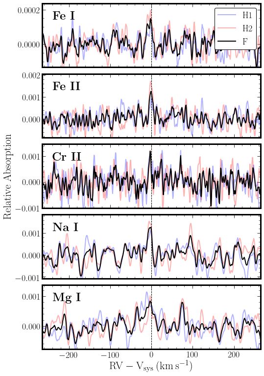
for clarity. the first half of transit (blue curve), second half (red curve) and
full transit (black curve), for each of the strongest species detec-
tions (Fe i, Fe ii and Cr ii). The legend denotes which in-transit
exposures were used in the calculation (H1, H2, F denote first
along random paths in the two-dimensional CCF. Results half of transit, second half of transit and full transit respec-
are shown in Figure 7, where the observed difference or tively). The dashed line indicates the expected location of the
greater occurs in 1.2×10⁻³ of all cases. Assuming the distri- signal, at 0.0 km s−1 velocity offset.
bution is Gaussian, the observed Fe ii amplitude difference
is at a 2.7σ confidence level.
Variability of the depth of absorption features has been dicative of a scale-height difference on both terminators,
observed in the transmission spectra of KELT-9 b (Cauley which could be caused by the temperature on the evening
et al. 2019) and currently most clearly in WASP-76 b terminator being higher than on the morning terminator.
(Ehrenreich et al. 2020). In the case of WASP-76 b, this is
attributed to differences in chemical composition between 4.2. Summary
the morning (leading) and evening (trailing) terminators,
due to the offset of the substellar hot-spot towards the In this paper we present detections of atomic metal ab-
evening terminator. These observations show the appear- sorption lines in the transmission spectrum of the ultra-hot
ance of a significant blue-shift as the evening twilight region Jupiter MASCARA-2 b (Lund et al. 2017; Talens et al.
rotates into view, which is explained by the rotation of the 2018). To this end, one transit of MASCARA-2 b was ob-
planet in combination with a day-to-night-side wind: The served with EXPRES, the high-resolution optical spectro-
transmission spectrum of the leading terminator probes graph newly commissioned at the Lowell Discovery Tele-
cool gas that streams from the night-side towards the hot scope. We confirm previous detections of Fe i, Fe ii and
day-side. Conversely, the trailing limb contains hot gas that Na i (Casasayas-Barris et al. 2018, 2019; Nugroho et al.
was strongly irradiated on the day-side and is approaching 2020; Stangret et al. 2020), and additionally find strong
the night-side where it cools down. However, in the case evidence for line absorption by atomic Mg i, and Cr ii. All
of M2 b, the absorption signal appears to be symmetric detected species appear to be blue-shifted, indicating the
around 0 km s−1 , which may indicate that the chemistry presence of a day-to-night side wind, also observed in pre-
at both terminators is more similar than for WASP-76 b. vious studies (e.g. Nugroho et al. 2020; Stangret et al.
An increase in the absorption line (which in this data may 2020). Using the shape variation of the stellar absorption
amount to a factor of 2, see Fig. 7), may however be in- lines induced by the transiting planet (i.e. the Doppler
Article number, page 9 of 20A&A proofs: manuscript no. main_arxiv
Allart, R., Bourrier, V., Lovis, C., et al. 2019, A&A, 623, A58
Allart, R., Lovis, C., Pino, L., et al. 2017, A&A, 606, A144
Astropy Collaboration, Robitaille, T. P., Tollerud, E. J., et al. 2013,
A&A, 558, A33
Birkby, J. L. 2018, arXiv e-prints, arXiv:1806.04617
Birkby, J. L., de Kok, R. J., Brogi, M., et al. 2013, MNRAS, 436, L35
Birkby, J. L., de Kok, R. J., Brogi, M., Schwarz, H., & Snellen, I. A. G.
2017, AJ, 153, 138
Blackman, R. T., Ong, J. M. J., & Fischer, D. A. 2019, AJ, 158, 40
Bourrier, V., Kitzmann, D., Kuntzer, T., et al. 2019, arXiv e-prints,
arXiv:1909.03010
Bourrier, V., Lecavelier des Etangs, A., Hébrard, G., et al. 2015, A&A,
579, A55
Brogi, M., de Kok, R. J., Albrecht, S., et al. 2016, ApJ, 817, 106
Brogi, M., Snellen, I. A. G., de Kok, R. J., et al. 2012, Nature, 486,
502
Cabot, S. H. C., Madhusudhan, N., Hawker, G. A., & Gandhi, S. 2019,
MNRAS, 482, 4422
Casasayas-Barris, N., Pallé, E., Yan, F., et al. 2018, A&A, 616, A151
Casasayas-Barris, N., Pallé, E., Yan, F., et al. 2019, A&A, 628, A9
Cauley, P. W., Shkolnik, E. L., Ilyin, I., et al. 2019, AJ, 157, 69
Cegla, H. M., Lovis, C., Bourrier, V., et al. 2016, A&A, 588, A127
Claudi, R., Benatti, S., Carleo, I., et al. 2017, European Physical
Journal Plus, 132, 364
Collier Cameron, A., Bruce, V. A., Miller, G. R. M., Triaud,
A. H. M. J., & Queloz, D. 2010, MNRAS, 403, 151
Cosentino, R., Lovis, C., Pepe, F., et al. 2012, Society of Photo-Optical
Instrumentation Engineers (SPIE) Conference Series, Vol. 8446,
Harps-N: the new planet hunter at TNG, 84461V
Fig. 7. Cumulative Distribution Function of the difference in Crossfield, I. J. M. 2015, PASP, 127, 941
amplitudes recovered from injecting an artificial Fe ii signal, and Delrez, L., Santerne, A., Almenara, J. M., et al. 2016, MNRAS, 458,
recovering it in the first and second halves of transit separately. 4025
Ehrenreich, D., Lovis, C., Allart, R., et al. 2020, Nature
The vertical blue line marks the measured difference in ampli- Evans, T. M., Sing, D. K., Goyal, J. M., et al. 2018, AJ, 156, 283
tudes. Fischer, D. A., Anglada-Escude, G., Arriagada, P., et al. 2016, PASP,
128, 066001
Flagg, L., Johns-Krull, C. M., Nofi, L., et al. 2019, ApJ, 878, L37
shadow), we constrain the projected spin-orbit misalign- Foreman-Mackey, D., Hogg, D. W., Lang, D., & Goodman, J. 2013,
ment to 1.6 ± 3.1 degrees, consistent with an aligned or- PASP, 125, 306
bit. The cross-correlation functions indicate hints of time- Gaudi, B. S., Stassun, K. G., Collins, K. A., et al. 2017, Nature, 546,
514
variability in the absorption strength of these species, albeit Grimm, S. L. & Heng, K. 2015, ApJ, 808, 182
at a level of . 3σ. With a single transit, we cannot rule out Guilluy, G., Sozzetti, A., Brogi, M., et al. 2019, A&A, 625, A107
that this variability is spurious. However, if it is astrophys- Hawker, G. A., Madhusudhan, N., Cabot, S. H. C., & Gandhi, S. 2018,
ical in origin, it potentially traces differential atmospheric ApJ, 863, L11
Heng, K. & Showman, A. P. 2015, Annual Review of Earth and Plan-
structure between morning and evening terminators, rem- etary Sciences, 43, 509
iniscent of what has recently been observed in the trans- Hoeijmakers, H. J., Ehrenreich, D., Heng, K., et al. 2018a, Nature,
mission spectrum of WASP-76 b (Ehrenreich et al. 2020). 560, 453
These results demonstrate the first spectroscopic observa- Hoeijmakers, H. J., Ehrenreich, D., Kitzmann, D., et al. 2019, A&A,
627, A165
tion of an exoplanet atmosphere with the EXPRES instru- Hoeijmakers, H. J., Snellen, I. A. G., & van Terwisga, S. E. 2018b,
ment, demonstrating its future potential for atmospheric A&A, 610, A47
characterisation. Husser, T.-O., Wende-von Berg, S., Dreizler, S., et al. 2013, A&A,
553, A6
Acknowledgements. This work was supported by the PlanetS Na- Jensen, A. G., Redfield, S., Endl, M., et al. 2012, ApJ, 751, 86
tional Centre of Competence in Research (NCCR) supported by the Khalafinejad, S., von Essen, C., Hoeijmakers, H. J., et al. 2017, A&A,
Swiss National Science Foundation (SNSF), the NSF under grants 598, A131
NSF MRI-1429365 and ATI-1509436 and by the European Re- search Levine, S. E., Bida, T. A., Chylek, T., et al. 2012, Society of Photo-
Council (ERC) under the European Union’s Horizon 2020 research Optical Instrumentation Engineers (SPIE) Conference Series, Vol.
and innovation programme (projects Four Aces and EXOKLEIN 8444, Status and performance of the Discovery Channel Telescope
with grant agreement numbers 724427 and 771620, respectively). We during commissioning, 844419
acknowledge generous support for telescope time provided by the Lockwood, A. C., Johnson, J. A., Bender, C. F., et al. 2014, ApJ, 783,
Heising-Simons Foundation and the Yale Astronomy Department. L29
DAF and JMB wish to acknowledge support from an anonymous do- Louden, T. & Wheatley, P. J. 2015, ApJ, 814, L24
nation, which has also been used for telescope time. LLZ gratefully Lund, M. B., Rodriguez, J. E., Zhou, G., et al. 2017, AJ, 154, 194
acknowledges support from the NSF GRFP. These results made use Madhusudhan, N., Agúndez, M., Moses, J. I., & Hu, Y. 2016,
of the Lowell Discovery Telescope at Lowell Observatory. Lowell is a Space Sci. Rev., 205, 285
private, non-profit institution dedicated to astrophysical research and Nugroho, S. K., Gibson, N. P., de Mooij, E. J. W., et al. 2020, arXiv
public appreciation of astronomy and operates the LDT in partnership e-prints, arXiv:2003.04856
with Boston University, the University of Maryland, the University of Nugroho, S. K., Kawahara, H., Masuda, K., et al. 2017, AJ, 154, 221
Toledo, Northern Arizona University and Yale University. We thank Ohta, Y., Taruya, A., & Suto, Y. 2005, ApJ, 622, 1118
the Lowell Observatory astronomers and staff for their extraordinary Oliva, E., Sanna, N., Rainer, M., et al. 2018, in Ground-based and
support. Airborne Instrumentation for Astronomy VII, ed. C. J. Evans,
L. Simard, & H. Takami, Vol. 10702, International Society for Op-
tics and Photonics (SPIE), 2118 – 2130
Pepe, F., Cristiani, S., Rebolo, R., et al. 2013, The Messenger, 153, 6
References Petersburg, R. R., Joel Ong, J. M., Zhao, L. L., et al. 2020, AJ, 159,
187
Albrecht, S., Winn, J. N., Johnson, J. A., et al. 2012, ApJ, 757, 18 Pino, L., Ehrenreich, D., Allart, R., et al. 2018, A&A, 619, A3
Article number, page 10 of 20H. Jens Hoeijmakers et al.: EXPRES Transmission Spectroscopy of MASCARA-2 b
Piskorz, D., Benneke, B., Crockett, N. R., et al. 2016, ApJ, 832, 131
Price-Whelan, A. M., Sipőcz, B. M., Günther, H. M., et al. 2018, AJ,
156, 123
Quirrenbach, A., Amado, P. J., Mandel, H., et al. 2010, Society of
Photo-Optical Instrumentation Engineers (SPIE) Conference Se-
ries, Vol. 7735, CARMENES: Calar Alto high-resolution search
for M dwarfs with exo-earths with a near-infrared Echelle spec-
trograph, 773513
Redfield, S., Endl, M., Cochran, W. D., & Koesterke, L. 2008, ApJ,
673, L87
Schlaufman, K. C. 2010, ApJ, 719, 602
Seidel, J. V., Ehrenreich, D., Wyttenbach, A., et al. 2019, A&A, 623,
A166
Showman, A. P., Fortney, J. J., Lewis, N. K., & Shabram, M. 2013,
ApJ, 762, 24
Smette, A., Sana, H., Noll, S., et al. 2015, A&A, 576, A77
Snellen, I. A. G., Albrecht, S., de Mooij, E. J. W., & Le Poole, R. S.
2008, A&A, 487, 357
Snellen, I. A. G., de Kok, R. J., de Mooij, E. J. W., & Albrecht, S.
2010, Nature, 465, 1049
Stangret, M., Casasayas-Barris, N., Pallé, E., et al. 2020, arXiv e-
prints, arXiv:2003.04650
Stock, J. W., Kitzmann, D., Patzer, A. B. C., & Sedlmayr, E. 2018,
MNRAS, 479, 865
Talens, G. J. J., Justesen, A. B., Albrecht, S., et al. 2018, A&A, 612,
A57
Thibault, S., Rabou, P., Donati, J.-F., et al. 2012, in Proc. SPIE, Vol.
8446, Ground-based and Airborne Instrumentation for Astronomy
IV, 844630
Thompson, S. J., Queloz, D., Baraffe, I., et al. 2016, in Society of
Photo-Optical Instrumentation Engineers (SPIE) Conference Se-
ries, Vol. 9908, Proc. SPIE, 99086F
Triaud, A. H. M. J. 2018, The Rossiter-McLaughlin Effect in Exo-
planet Research, 2
Turner, J. D., de Mooij, E. J. W., Jayawardhana, R., et al. 2020, ApJ,
888, L13
Wildi, F., Blind, N., Reshetov, V., et al. 2017, in Society of Photo-
Optical Instrumentation Engineers (SPIE) Conference Series, Vol.
10400, Society of Photo-Optical Instrumentation Engineers (SPIE)
Conference Series, 1040018
Winn, J. N., Fabrycky, D., Albrecht, S., & Johnson, J. A. 2010, ApJ,
718, L145
Wright, J. T. 2018, Radial Velocities as an Exoplanet Discovery
Method, 4
Wyttenbach, A., Ehrenreich, D., Lovis, C., Udry, S., & Pepe, F. 2015,
A&A, 577, A62
Wyttenbach, A., Lovis, C., Ehrenreich, D., et al. 2017, A&A, 602, A36
Yan, F. & Henning, T. 2018, Nature Astronomy, 2, 714
Article number, page 11 of 20A&A proofs: manuscript no. main_arxiv Appendix A: MCMC Results, Additional Figures Article number, page 12 of 20
H. Jens Hoeijmakers et al.: EXPRES Transmission Spectroscopy of MASCARA-2 b

          Parameter                                Symbol        Unit      MCMC Median          T18 (Prior)            L17
          Scaled Semi-major Axis                    a/R∗          -          7.50 ± 0.04        7.50 ± 0.04       7.44+0.14
                                                                                                                      −0.13
          Projected Obliquity                         λ            ◦
                                                                               1.58+3.14
                                                                                   −3.12            0.6 ± 4       3.4 ± 2.1
          Orbit Inclination                           ip           ◦
                                                                             86.16 ± 0.5           86.4+0.5
                                                                                                       −0.4      86.15+0.28
                                                                                                                      −0.27
          Projected Stellar Rotation Speed         v sin i∗    km s−1        113.50+0.77
                                                                                   −0.74            114 ± 3     115.9 ± 3.4
          RV Offset                                    -       km s−1          0.7 ± 3.1             0 ± 5∗               -
Table A.1. MCMC results for modelling of the Rossiter-McLaughlin effect. The model consists of the four parameters listed in
column one, plus a global RV offset. The MCMC median values are listed in column four. Uncertainties correspond to the 16th
and 84th percentiles. For comparison, we list literature values in column five, and their references in column 6. T18 denotes Talens
et al. (2018), and L17 denotes Lund et al. (2017). Asterisk (∗ ) indicates RV Offset prior not from literature.

Fig. A.1. Correlation diagram from our MCMC fit to the observed Doppler shadow, as well as one-dimensional histograms. The
model consists of five parameters: scaled semi-major axis (a/R∗ ), projected obliquity (λ), orbital inclination (ip ), projected stellar
rotation speed (v sin i∗ ), and a global RV offset. Red lines denote literature values for the parameters (Talens et al. 2018).

                                                                                                        Article number, page 13 of 20
A&A proofs: manuscript no. main_arxiv Fig. A.2. Same as Figure 4, depicting the cross-correlation process for Fe i. CCFs are in the rest-frame of the planet. Fig. A.3. Same as Figure 4, depicting the cross-correlation process for Ti i. CCFs are in the rest-frame of the planet. Article number, page 14 of 20
H. Jens Hoeijmakers et al.: EXPRES Transmission Spectroscopy of MASCARA-2 b

Fig. A.4. Same as Figure 4, depicting the cross-correlation process for Ti ii. CCFs are in the rest-frame of the planet.

Fig. A.5. Same as Figure 4, depicting the cross-correlation process for Cr i. CCFs are in the rest-frame of the planet.

                                                                                                    Article number, page 15 of 20
A&A proofs: manuscript no. main_arxiv Fig. A.6. Same as Figure 4, depicting the cross-correlation process for Cr ii. CCFs are in the rest-frame of the planet. Fig. A.7. Same as Figure 4, depicting the cross-correlation process for Sc i. CCFs are in the rest-frame of the planet. Article number, page 16 of 20
H. Jens Hoeijmakers et al.: EXPRES Transmission Spectroscopy of MASCARA-2 b

Fig. A.8. Same as Figure 4, depicting the cross-correlation process for Sc ii. CCFs are in the rest-frame of the planet.

Fig. A.9. Same as Figure 4, depicting the cross-correlation process for Y ii. CCFs are in the rest-frame of the planet.

                                                                                                    Article number, page 17 of 20
A&A proofs: manuscript no. main_arxiv Fig. A.10. Same as Figure 4, depicting the cross-correlation process for Na i. CCFs are in the rest-frame of the planet. Fig. A.11. Same as Figure 4, depicting the cross-correlation process for Mg i. CCFs are in the rest-frame of the planet. Article number, page 18 of 20
H. Jens Hoeijmakers et al.: EXPRES Transmission Spectroscopy of MASCARA-2 b

Fig. A.12. Same as Fig 5, except based on cross-correlation with the Fe i template. This plot shows the distribution of strengths
of random signals generated by the CCFs, from which the FAP is derived.

Fig. A.13. Same as Fig 5, except based on cross-correlation with the Cr ii template. This plot shows the distribution of strengths
of random signals generated by the CCFs, from which the FAP is derived.

                                                                                                    Article number, page 19 of 20
A&A proofs: manuscript no. main_arxiv Fig. A.14. Same as Fig 5, except based on cross-correlation with the Na i template. This plot shows the distribution of strengths of random signals generated by the CCFs, from which the FAP is derived. Fig. A.15. Same as Fig 5, except based on cross-correlation with the Mg i template. This plot shows the distribution of strengths of random signals generated by the CCFs, from which the FAP is derived. Article number, page 20 of 20
You can also read