Hyperspectral imaging with a TWINS birefringent interferometer

Vol. 27, No. 11 | 27 May 2019 | OPTICS EXPRESS 15956

Hyperspectral imaging with a TWINS
birefringent interferometer
A. PERRI,1,2,4 B. E. NOGUEIRA DE FARIA,3,4 D. C. TELES FERREIRA,3 D.
COMELLI,1 G. VALENTINI,1 F. PREDA,1,2 D. POLLI,1,2 A. M. DE PAULA,3 G.
CERULLO,1,2 AND C. MANZONI1,*
1
  IFN-CNR, Dipartimento di Fisica, Politecnico di Milano, Piazza Leonardo da Vinci 32, I-20133
Milano, Italy
2
  NIREOS S.R.L., Via G. Durando 39, 20158 Milano, Italy
3
  Departamento de Física, Universidade Federal de Minas Gerais, 31270-901 Belo Horizonte-MG,
Brazil
4
  The authors contributed equally to the work
*cristian.manzoni@polimi.it

Abstract: We introduce a high-performance hyperspectral camera based on the Fourier-
transform approach, where the two delayed images are generated by the Translating-Wedge-
Based Identical Pulses eNcoding System (TWINS) [Opt. Lett. 37, 3027 (2012)], a common-
path birefringent interferometer that combines compactness, intrinsic interferometric delay
precision, long-term stability and insensitivity to vibrations. In our imaging system, TWINS
is employed as a time-scanning interferometer and generates high-contrast interferograms at
the single-pixel level. The camera exhibits high throughput and provides hyperspectral
images with spectral background level of −30dB and resolution of 3 THz in the visible
spectral range. We show high-quality spectral measurements of absolute reflectance,
fluorescence and transmission of artistic objects with various lateral sizes.

© 2019 Optical Society of America under the terms of the OSA Open Access Publishing Agreement

1. Introduction
A great deal of physico-chemical information on objects can be obtained by measuring the
spectrum of the light they emit, scatter or reflect. Spectral imaging, also known as imaging
spectroscopy [1], refers to a set of methods and devices for acquiring the light spectrum for
each point in the image of a scene. Among them, hyperspectral imaging (HSI) [2] acquires
the full continuous spectrum of light for each point (x,y) of the scene, resulting in a three-
dimensional data-cube as a function of (x,y,ω), where ω is the frequency. Starting from the
spectral information, numerical methods enable extracting quantitative parameters related to
chemical and physical properties of the imaged objects [3,4]. HSI is a powerful technique for
a wide range of fundamental and applied studies in fields as diverse as remote sensing [5,6],
medical imaging [7], agriculture [8,9], coastal and geological prospecting [10,11], safety and
security [12], archaeology [13,14] and conservation science [15]. HSI has been implemented
in a wide variety of methods [1]. The most straightforward approaches are Snapshot HSI [16]
which uses a mosaic of bandpass filters on the detector surface, and spectral (or staring) HSI,
which uses a tunable spectral filter in front of a monochrome imaging camera [17]. However,
these techniques only enable acquisition of a discrete number of bands. To measure
continuous spectra, a common method is spatial scanning HSI, which combines a dispersive
spectrometer with a raster-scanning approach, either in point scanning (whisk-broom) or line
scanning (push-broom) modes. This technique is currently implemented in most commercial
HSI systems, but the high losses imposed by the entrance slit of the spectrometer lead to long
acquisition times.
    An alternative HSI method combines a monochrome imaging camera with a Fourier-
transform (FT) spectrometer [18]. In FT spectroscopy an optical waveform is split in two

#357421                                                                 https://doi.org/10.1364/OE.27.015956
Journal © 2019       Received 11 Jan 2019; revised 3 May 2019; accepted 14 May 2019; published 21 May 2019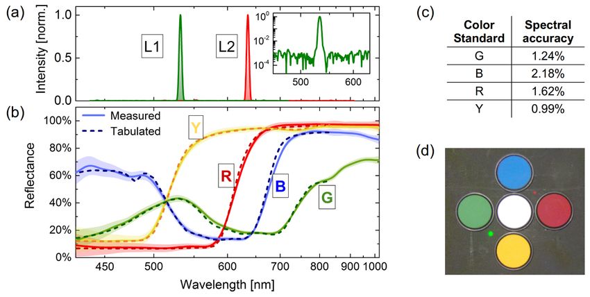

Vol. 27, No. 11 | 27 May 2019 | OPTICS EXPRESS 15957

collinear delayed replicas, whose interference pattern is measured by a detector as a function
of their delay. The FT of the resulting interferogram yields the continuous-intensity spectrum
of the waveform. FT spectrometers have prominent advantages over dispersive ones: (i)
higher signal-to-noise ratio in a readout-noise-dominated regime (the Fellgett multiplex
advantage [19]); (ii) higher throughput, due to the absence of slits (the Jacquinot étendu
advantage [20]); (iii) flexible spectral resolution, which is adjusted at will by varying the
maximum scan delay; (iv) possibility of parallel recording of the spectra of all pixels within a
two-dimensional scene of an imaging system.
    A FT-based imaging system must fulfil two key requirements: (i) the delay of the replicas
must be controlled to within a fraction (1/100 or better) of the optical cycle (e.g., 0.02 fs at
600 nm); (ii) the bundle of rays that form the interferogram at a given pixel must have a high
degree of coherence. This last requirement guarantees visibility of the interference fringes,
which is one of the most important criteria for evaluating the performance of an interference
imaging spectrometer, as it determines the quality of the retrieved spectrum of a scene, and is
essential for spectroscopic analysis with high accuracy. FT-based imaging is achieved using
either a static or a temporal approach. In the static scheme, the interferometer has no moving
parts, and a spatial interferogram is formed along one of the dimensions of the image. The
acquisition is performed by moving the object with respect to the camera [21], making this
method particularly suited in production lines, in which the object to be measured is moving
e.g. on a conveyor belt, or for airborne remote sensing. In the temporal approach, the
interferometer is scanned in order to vary the delay of the replicas, with no need of relative
movement between the object and the camera. This method is better suited for the imaging of
stationary objects. FT HSI systems have been built based on Michelson or Mach-Zehnder
interferometers [22]; however, since they are sensitive to vibrations, it is difficult to achieve
the required interferometric stability without active stabilization or tracking. Alternatively,
liquid crystal cells have been used to introduce a voltage-controlled delay between orthogonal
polarizations [23–25]. In the last few years, birefringent interferometers have attracted
particular attention because of their compactness and insensitivity to vibrations, due to their
common-path nature. They are mostly based on Wollaston or Savart prisms [26,27], or their
variants [28]; because of the arrangement of their optical axes, they are characterized by a
strong chromatic lateral displacement, which reduces the visibility of the interference fringes
[29].
    Recently we introduced the Translating-Wedge-based Identical pulses eNcoding System
(TWINS) [30,31], a common-path birefringent interferometer inspired by the Babinet–Soleil
compensator, but conceived to provide retardation of hundreds of optical cycles between two
orthogonal polarizations of a light beam. Thanks to the favorable arrangement of the optical
axes, the light replicas in TWINS are collinear, with no lateral displacement, thus
guaranteeing very high contrast of the interference fringes. In addition, as the two fields share
a common optical path, their delay is adjusted with interferometric precision, with
fluctuations as small as 1/360 of the optical cycle without any active stabilization or tracking
[30]. The TWINS interferometer has been successfully employed as a FT spectrometer in
spectral ranges from the visible [32,33] to the mid-infrared [34,35], with both coherent and
incoherent light beams.
    In this paper we introduce a compact, low-cost hyperspectral camera using the temporal
FT approach, in which the interferometer is based on the simplified version the birefringent
TWINS device [32,33]. Our approach combines the advantages of FT HSI with the
robustness, accuracy and high contrast of TWINS. We demonstrate that TWINS applied to
FT imaging provides a high degree of coherence at each pixel of the image. This enables HSI
with short acquisition times, high spectral accuracy, and background level of only −30dB.
The simplicity of our experimental configuration combined with the high spatial and spectral
quality of the data-cube promise to broaden the application fields of HSI.

Vol. 27, No. 11 | 27 May 2019 | OPTICS EXPRESS 15958

2. The TWINS-based hyperspectral camera
2.1. Experimental setup
A scheme of the hyperspectral camera is shown in Fig. 1. It consists of a TWINS
interferometer (P1, A, B and P2) followed by a monochrome imaging system.

         Fig. 1. Schematic setup of the hyperspectral camera. P1 and P2: wire-grid polarizers; A block:
         α-BBO wedges, with optical axis parallel to the plane (green double arrow); B block: α-BBO
         plate, with optical axis normal to the plane (green circle). The brown double arrow indicates
         the wedge translation direction. O: object; I: image.

    A and B are birefringent blocks made of α-barium borate (α-BBO), P1 and P2 are wire-
grid polarizers with extinction ratio >5000 at wavelengths from 400 nm to 2 μm. P1 polarizes
the input light at 45° with respect to the optical axes of A and B. Block B is a plate with
thickness L = 2.4 mm and aperture diameter D = 5 mm; it introduces a fixed phase delay
between the two orthogonal polarizations that propagate along the fast and slow axes of the
material. Block A has optical axis orthogonal to the one of block B (see green arrows and
circle in Fig. 1, respectively), thus applying a delay with opposite sign. The overall phase
delay introduced by the TWINS ranges from positive to negative values according to the
relative thickness of the two blocks. To enable fine tuning of the phase delay, block A is
shaped in the form of two wedges with the same apex angle (7°), one of which is mounted on
a motorized translation stage (L-402.10SD, Physik Instrumente) with maximum travel range
of 13 mm. Interference between the two replicas is guaranteed by P2, which is also set at 45°
with respect to the optical axes of A and B, and projects the two fields to the same
polarization. The spectral resolution of the interferometer is inversely proportional to the total
phase delay. For example, scanning the position of the wedges ± 1mm around the zero path
delay (ZPD) introduces a delay of ± 50 fs to the replicas of a wave at λ = 600 nm; this
corresponds to spectral resolution of 15 THz (~18 nm). The camera lens has focal length f =
25 mm and maximum aperture f/1.4. The detector is a monochrome CMOS silicon camera
with size 6.78 mm × 5.43 mm (1/1.8” format), 1280 × 1024 pixels, with 10-bits depth and
spectral sensitivity from 400 nm to 1100 nm. The total angular field of view of the combined
camera lens and detector is 15.4° (19° along the sensor diagonal).
2.2. Imaging capability of the TWINS interferometer
In the following, we will show under which conditions our TWINS birefringent
interferometer enables performing FT spectral imaging. In general, an imaging system must
maintain coherence (i.e., similar path delay) between the rays of the bundle that form the
interferogram at a given pixel. To this aim, we will follow the pencil of rays propagating from
one object point O to the detector surface of our camera, and we will calculate the relative
phase they accumulate due to the interferometer.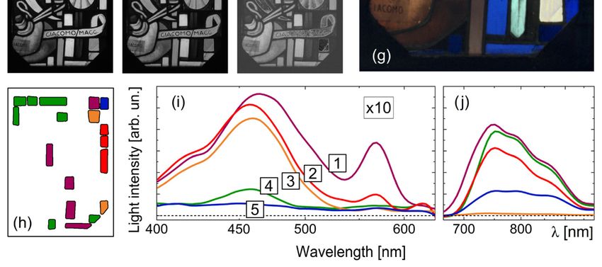

Vol. 27, No. 11 | 27 May 2019 | OPTICS EXPRESS 15959

         Fig. 2. (a) Top view of the optical paths and refractive indexes of the vertically-polarized (V,
         red) and horizontally-polarized (H, blue) components of a ray traveling in the TWINS system;
         dashed lines: extraordinary (e) rays; solid lines: ordinary (o) rays. Air spacing between the
         surfaces has been removed for simplicity. (b) Relative phase accumulated by the cross-
         polarized components as a function of α. (c) Visibility of the interferogram of a CW wave, as a
         function of the phase spread Δφ. Vertical lines correspond to various distances h of an object at
         the edge of the field of view of our camera. Inset: definition of v. (d) Diagram of two marginal
         rays (1 and 2) propagating from the sources point O to the image point I; φ1, φ2: relative phase
         between the vertically- and horizontally-polarized components of the field replicas.

    Figure 2(a) shows the path of one generic ray impinging at angle α onto two birefringent
plates with orthogonal optical axes. The plates mimic blocks A and B of the TWINS
interferometer; we consider the case in which they have the same thickness L, i.e. the nominal
delay T of the interferometer is set to 0. Due to birefringence, the beam splits into two
orthogonally polarized replicas, which travel along different optical paths. The ordinary
beams experience the same ordinary index no, while the extraordinary beams experience ne(α)
and ne in blocks A and B respectively. As a consequence, at the output of the interferometer
the horizontally-polarized component of the field (blue) is phase-shifted by φ with respect to
the vertically-polarized one (red). The dependence of φ on α, calculated without loss of
generality at the working conditions of our interferometer (λ = 600 nm, in α-BBO crystal with
L = 2.4 mm), is shown in Fig. 2(b). The rays of a bundle typically impinge onto the
interferometer at various angles around α0, with range Δα; hence their phase shifts vary within
Δφ. Such a phase span leads to a reduction of the fringe visibility v at the image point. To
evaluate v, let’s consider the two replicas of a generic i-th ray of the bundle at frequency ω. In
the frame of reference of the vertically polarized beam and in the neighborhood of T = 0, they
can be written as:
                                 Ei = Ai ⋅{cos[ωt ] + cos[ω (t − T ) − ϕi ]}.                                (1)

The overlap at the image pixel I of all rays from O (see Fig. 2(d)) results in EI (T ) =  i Ei .
By taking the summation, we obtain that the resulting interferogram intensity I = Ei (T )2
depends on the distribution of phase shifts φi. In the worst-case assumption that all rays have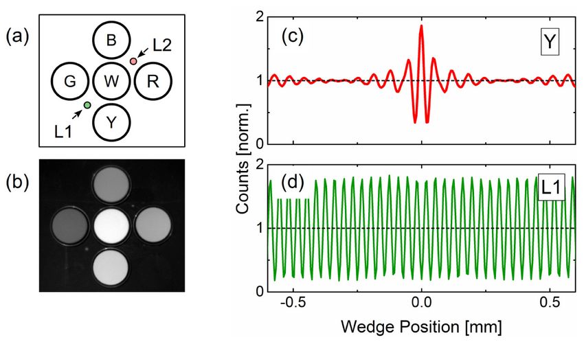

Vol. 27, No. 11 | 27 May 2019 | OPTICS EXPRESS 15960

the same amplitude Ai and their phase φi uniformly spans within Δφ, the visibility v of
 Ei (T )2 calculated as a function of Δφ is shown in Fig. 2(c).
   With these general concepts, we can now estimate the fringe visibility expected from our
hyperspectral camera. Figure 2(d) schematically sketches its essential optical elements, along
with the path of the light from one object point O to the corresponding image point I; the
object is at angle α0, and the incidence angles α of its pencil of rays range from α1 to α2, where
1 and 2 are the marginal rays. According to Fig. 2(d), the range Δα is:
                                                    D/h
                       Δα = α1 − α 2 ≈ arc tan                 < arc tan( D / h).               (2)
                                                 1 + tan 2 α 0

which is broader when the object is closer to the camera. The corresponding phase shifts
range from φ1 = φ(α1) to φ2 = φ(α2).
    Let’s now focus on the object points with the worst fringe visibility, i.e. the ones
accumulating the largest value of Δφ at the image pixel. Since Δφ is, to the first order, the
product between Δα and the slope of the curve φ(α), larger values of Δφ are obtained where
the slope of the curve φ(α) is the steepest, i.e. at the edge of the field of view (see Fig. 2(b))
and for large values of Δα, i.e. when the object is close to the camera lens (see Eq. (2)). In the
case of our camera, an object placed at the edge of the field of view is at α0 = 7.7°. The
amplitudes of Δφ and the corresponding visibility calculated for various distances h from the
camera lens are shown in Fig. 2(c) as dashed vertical lines. The calculation demonstrates that
the camera is expected to provide visibility larger than 85% at all pixels for objects farther
than 0.5m from the camera lens. At shorter distances, the visibility slowly vanishes,
especially at the edge of the field of view. The high visibility demonstrates that our scheme is
well suited for FT HSI.
3. Characterization of the camera performances
The hyperspectral camera was tested for the analysis of various objects, with variable
properties and lateral size. In all cases we performed single-sweep acquisitions, moving the
translation stage with nominal steps of 5 μm, and took a single-exposure image at each delay.
The total length of the scan was adjusted to achieve the desired spectral resolution. Note that
the sampling step corresponds to a phase delay of 0.25 fs at λ = 600 nm, equivalent to 1/8 of
the optical cycle; this oversampling with respect to the Nyquist limit enables improving the
S/N ratio of the acquisition. To demonstrate that the TWINS interferometer is able to measure
spectra with high accuracy, we imaged a test scene made of a set of calibrated spectral
standards, as shown in Figs. 3(a) and 3(b): the test scene consists of 4 colored Spectralon
materials (green, blue, red, yellow, G, B, R, Y), acting as calibrated diffusive reflectance
standards (Labsphere Inc., North Sutton, USA), and a white Spectralon (W), with (98.3 ±
1.3)% reflectance in the range from 300 nm to 2.5 μm (Labsphere Inc.); each of them has
diameter of 1 inch. In addition, the beams of a green (λ = 532 nm) and a red diode laser (λ =
635 nm), both with bandwidth of 0.37 THz, were directed on points L1 and L2 respectively.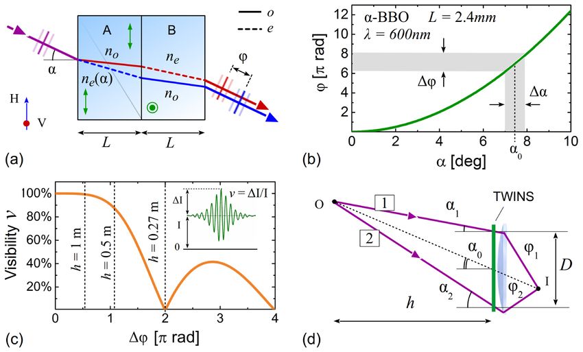

Vol. 27, No. 11 | 27 May 2019 | OPTICS EXPRESS 15961

         Fig. 3. (a) Geometrical arrangement and (b) intensity single-exposure image of the test object,
         taken at delay position of 1 mm (the complete temporal data cube as an animation is shown in
         the associated Visualization 1). G, B, R, Y: Spectralon diffuse color standards; W: Spectralon
         white standard; L1/L2: beam spots of diode lasers at λ = 532 nm/635 nm. (c) Single-scan
         interferogram of one image point at the surface of the Y color standard and (d) at L1.

     The scene was illuminated by a broadband 150W Xenon lamp. The camera lens was set at
its largest aperture and the integration time for each snapshot was only 25 ms. We scanned
the position of the wedges ± 1mm around the ZPD, corresponding to a total of 400 images.
The acquisition of the data-cube, including lapse time for motor movement and data transfer,
required less than 30 seconds. This acquisition time could be further reduced by optimizing
the digital communication with the camera and by sampling with longer steps to reduce the
number of images (eventually employing undersampling strategies). Figures 3(c) and 3(d)
show a portion of the raw interferograms of two pixels, on the region of the Y colored
standard and on the L1 area. The fringe visibility of the two interferograms is 86.5% and 84%
respectively. The high contrast proves that, when placed before the camera lens, the TWINS
interferometer provides high degree of coherence at the single-pixel level, as required by FT
HSI. Note that high contrast also reduces the spectral background noise, since the
contribution to the noise of the A/D conversion of the interferogram is inversely proportional
to the visibility [36]. The high contrast can be further improved by closing the lens aperture,
at the cost of reducing the light flux on the detector.
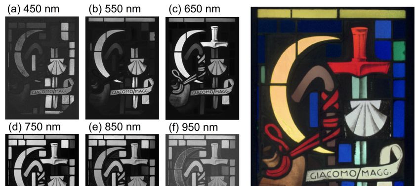
3.1. Frequency calibration and resolution
The narrowband green (λ = 532 nm) and red (λ = 635 nm) diode laser spots in L1 and L2
enable the spectral characterization of the camera. Figure 4(a) shows their resulting
normalized spectra. From their acquisition, the following information can be obtained:
(i) the positions of their spectral peaks enable the calibration of the frequency axis of the FT
      spectrometer [30,32];
(ii) their bandwidth provides the spectral resolution of the interferometer which, for ± 5-mm
      scan, is 3THz (~4 nm at λ = 635 nm), corresponding to 1/150 of the spectral range of the
      camera. For this high-resolution measurement, we acquired 1000 images with nominal
      sampling steps of 10 μm, and the acquisition required 95 seconds;
(iii) the interferogram (see Fig. 3(d) for L1) allows retrieving with sub-cycle precision the
      true delay of the interferometer during the scan. The detailed description of the technique
      and the measured deviation from the expected wedge position are reported in the
      Appendix section. By using the measured positioning for the FT calculation, the spectral
      background level is 30dB lower than the peak, as shown in the inset of Fig. 4(a). Note
      that this self-calibration procedure, which simply requires shining laser light in a small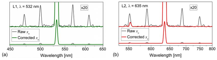

Vol. 27, No. 11 | 27 May 2019 | OPTICS EXPRESS 15962

    part of the scene (e.g. L1 and/or L2), is an effective alternative to internal encoders or
    feedback systems.

         Fig. 4. (a) Measured spectra of lasers L1 and L2 (position scan: ± 5 mm around the ZPD).
         Inset: spectrum of L1 in log scale. (b) Tabulated(dashed lines) and measured (solid lines)
         reflectance spectra of the color standards (position scan: ± 1 mm around the ZPD); shaded
         areas: wavelength-dependent standard deviations of the spectra measured over all points of
         each color standard surface; (c) spectral accuracy of the hyperspectral image of the color
         standards; (d) RGB image generated from the hyperspectral data-cube.

   We observed that neither the frequency calibration of point (i) nor the retrieved true delay
of point (iii) change from day to day; the frequency and phase delay calibration must be
repeated only when the alignment of one or more birefringent elements is changed.
3.2. Absolute reflectivity measurements
Figure 4(b) shows the reflectance spectra of the diffusive colorimetric standards, and
summarizes the accuracy of the hyperspectral camera in retrieving absolute spectral
information. The dashed lines are the certified reflectivity values, while the solid lines are the
spectra retrieved from our HSI system and averaged over the surface of each standard.
Absolute reflectance was calculated after spectral calibration with the white Spectralon W and
correction for spatial and spectral non-uniformities of the illumination by imaging a white
Lambertian surface at the object plane (data not shown). The spectral accuracy for each
colorimetric sample, estimated as the standard deviation of the difference between measured
and certified spectra, is reported in Fig. 4(c). The difference is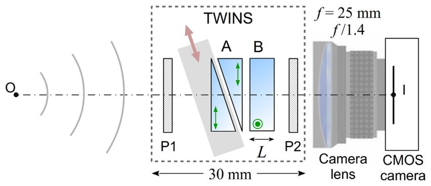

Vol. 27, No. 11 | 27 May 2019 | OPTICS EXPRESS 15963

optical emission of the sample, upon excitation with a broadband LED around λ = 617 nm
and with exposure time of 700ms per image. The measured fluorescence spectrum, shown in
Fig. 5(c) as a shaded area, is in excellent agreement with literature [37]. Figure 5(b) shows the
image of the intensity of the emission at 900 nm, which reveals the presence of Egyptian Blue
in some of the decorations.

         Fig. 5. Hyperspectral imaging of the Egyptian cartonnage (size ~18cm × 16cm). (a) RGB
         image synthesized from the hyperspectral data. (b) False-color fluorescence image at λ = 900
         nm after illumination at λ = 617 nm. (c) Solid/dashed lines: Reflectance spectra of three points
         of panel (a); shaded area: fluorescence spectrum (the full-resolution RGB and fluorescence
         images are shown in Visualization 2).

    Finally, we demonstrate HSI of a stained glass window, whose plates typically exhibit
strong absorption bands located at well-defined wavelengths. Since window glass
manufacturing has changed throughout time, spectral characterization is a means to determine
the composition of glasses and of their coloring agents, to assess the authenticity of ancient
windows [39].

         Fig. 6. Hyperspectral imaging of an artistic glass window (A. M. Nardi, 1969). (a-f) Subfigures
         from the data-cube, at selected wavelengths (the complete spectral data cube as an animation is
         shown in the associated Visualization 3). (g) Color image synthesized from the spectral data
         (the full-resolution RGB image is shown in Visualization 4); (h) map and (i,j) corresponding
         transmitted spectra of the blue tiles, after automatic image segmentation; spectra in the visible
         range (i) are rescaled by a factor of 10.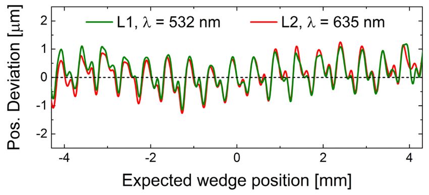

Vol. 27, No. 11 | 27 May 2019 | OPTICS EXPRESS 15964

    Figure 6 shows the results from HSI of a portion of an artistic glass window at Santo
Spirito Church in Milan (Italy), designed in 1969 by A. M. Nardi (1897-1973). The window
was back-illuminated by natural sunlight, and the camera recorded the transmitted light;
exposure time was 100ms per image, and we acquired 400 images ( ± 1-mm scan). From the
data-cube, we extracted a subset of images at selected wavelengths (Figs. 6(a)–(f)); as
expected, each tile absorbs at specific spectral bands. The synthesized RGB color image is
shown in Fig. 6(g). We observed that tiles with similar colors exhibit different transmission
spectra. Automatic image k-means segmentation of the blue tiles [40] allows their separation
into 5 classes with distinct spectral transmission (Figs. 6(h)–(j)) and hence material
composition, despite their similar visual appearance. In particular, we identified two blue tiles
(cluster 3) with negligible infrared transmission.
5. Conclusions
In conclusion, we have introduced an HSI system using a common-path birefringent
interferometer, the TWINS, to perform FT imaging. Our configuration shares the main
advantages of FT spectroscopy, such as high light throughput due to the absence of slits, the
multiplexing advantage and the user adjustable spectral resolution. The use of the TWINS
adds several key advantages: (i) exceptional delay precision and long-term stability; (ii)
insensitivity to vibrations, making it suitable for hand-held devices; (iii) low cost and
simplicity. We have demonstrated that our compact hyperspectral camera is able to acquire
spectral absolute reflectance, transmittance and fluorescence images with broad spectral
coverage (400 THz) and high spectral resolution (3 THz), which can be easily increased by
the use of thicker birefringent plates. The angular field of view (15.4°, set by the f = 25 mm
camera lens) can be easily increased by employing camera lenses with shorter focal lengths
and using larger plates to avoid vignetting. Thanks to the high interferometric visibility and
the throughput offered by our camera the acquisition time of each frame is as short as 10 ms
with low-dose illumination by a 150 W Xenon lamp. While our present configuration covers
the 400-1000 nm range of silicon detectors, it can be straightforwardly extended to the short-
wavelength infrared and mid-infrared ranges using suitable detectors and birefringent
materials (such as LiNbO3 and Hg2Cl2), enabling a broad range of imaging and sensing
applications.
Appendix: Detection and correction of the delay axis
The FT approach is very sensitive to the exact positioning of the delay line. Deviations from
the expected delay may be due to various factors, such as imperfections in the interferometer
delay line, or perturbations during the measurement. For this reason, precise measurement of
the delay is essential for the correct calculation of the FT. In our camera, the delay can be
characterized simply by shining narrowband laser beams on a small area of the scene (e.g. at
the edge of the image), and analyzing their interferogram.
    The interferogram of a monochromatic light is a pure cosine function. In its general form,
it can be written as:
                                          yn = cos(a ⋅ xn ).                                      (3)

where a is the cosine angular frequency and xn is the generic interferometer position at the
sampling step n . Conceptually, from the measured interferogram yn of a monochromatic
light it is possible to extract the true interferometer position xn ; the most straightforward and
accurate method is based on the Fourier transform approach. In fact, Eq. (3) can be written as:
                                        1              1
                                    yn = ei ( a⋅ xn ) + e−i ( a⋅ xn ) .                           (4)
                                        2              2

Vol. 27, No. 11 | 27 May 2019 | OPTICS EXPRESS 15965

By taking the Fourier transform of yn and then back-transforming only the spectrum at
positive frequencies, one isolates the first exponential, obtaining the complex function:
                                                    1
                                               y n = ei ( a⋅ xn ) .                                       (5)
                                                    2
in which the exact interferometer position xn is proportional to the phase of yn .
    We applied this approach to estimate the position deviation of our birefringent
interferometer. To this aim, we shone the two narrowband diode laser beams on areas L1 and
L2 of the scene. To retrieve the positioning deviation over the broadest excursion of the
interferometer, and estimate its effects on the retrieved FT, here we analyze the long
interferograms of L1 and L2 obtained after scanning the wedge position ±5-mm around the
ZPD.

        Fig. 7. Deviation of the interferometer delay from its ideal position, deduced from the
        interferogram of image areas at L1 (green line) and L2 (red line).

    Figure 7 shows the deviation of the retrieved position xn of the interferometer from its
expected coordinate, deduced by analyzing independently the interferograms of image areas
at L1 (green line) and L2 (red line). The two lines, which are in excellent agreement, show
that the deviation is cyclic with remarkably low fluctuations: the maximum excursion is only
±1 μm, corresponding to 1/40 of the L2 laser optical cycle. Repeated measurements showed
reproducible deviations, demonstrating the robustness and reproducibility of our
interferometer. The fluctuations can mainly be attributed to imperfections of the delay line
and the wedges, while external perturbations are negligible.
    The retrieved position xn can be applied to correct the interferograms during FT data
analysis, by means of non-uniform Fourier transform algorithms. To show how positioning
deviations affect the calculated spectra, we applied the average of the deviations shown in
Fig. 7 for the calculation of the spectra of L1 and L2.

        Fig. 8. Spectra of the L1 (a) and L2 (b) lasers. Black lines: FT has been performed taking into
        account only the expected motor position. Red/green lines: FT has been performed taking into
        account the measured motor position, which is used to correct the interferogram. The spectra
        of each panel are also expanded by 20 × for clarity.

Vol. 27, No. 11 | 27 May 2019 | OPTICS EXPRESS 15966

    The results are shown in Fig. 8. The spectra in black line have been obtained by
considering the expected motor positioning; the cyclic position deviation results in sidebands,
with intensities of 1/20 of the peak. The green and red lines are the spectra obtained after
taking into account the average of the retrieved positions; in this case, the sidebands are
almost completely suppressed, and the background level is at −30dB (see inset of Fig. 4(a)).
Funding
Capes (process CSF-PVE-S-88881.068168/2014-01); Fapemig; CNPq; ERC PoC FLUO
(process 825879); Graphene Flagship (785219 GrapheneCore 2).
Acknowledgments
BENF, DCTF, AMdP and CM acknowledge financial support from the Brazilian funding
agencies Capes (process CSF-PVE-S-88881.068168/2014-01), Fapemig and CNPq. DP, FP
and GC acknowledge financial support from ERC PoC FLUO (process 825879). GC
acknowledges financial support from the Graphene Flagship (785219 GrapheneCore 2).
Authors wish to thank C. Orsenigo (Università degli studi di Milano), F. Moruzzi and M.
Facchi (Museo civico di Crema e del Cremasco), and A. Boni (Comune di Crema) for
providing access to the antiquities collection of the late Carla Maria Burri (1935–2009)
conserved at the Museo Civico di Crema e del Cremasco.
References
1.    W. L. Wolfe, Introduction to Imaging Spectrometers (SPIE, 1997).
2.    M. T. Eismann, Hyperspectral Remote Sensing (SPIE, 2012).
3.    H. F. Grahn and P. Geladi, Techniques and Applications of Hyperspectral Image Analysis (John Wiley & Sons,
      2007).
4.    J. M. Amigo, H. Babamoradi, and S. Elcoroaristizabal, “Hyperspectral image analysis. A tutorial,” Anal. Chim.
      Acta 896, 34–51 (2015).
5.    E. Ben-Dor, T. Malthus, A. Plaza, and D. Schlapfer, Airborne Measurements for Environmental Research:
      Methods and Instruments (Wiley, 2013), Chap 8.
6.    R. G. Sellar and G. D. Boreman, “Classification of imaging spectrometers for remote sensing applications,” Opt.
      Eng. 44(1), 013602 (2005).
7.    G. Lu and B. Fei, “Medical hyperspectral imaging: a review,” J. Biomed. Opt. 19(1), 010901 (2014).
8.    L. M. Dale, A. Thewis, C. Boudry, I. Rotar, P. Dardenne, V. Baeten, and J. A. F. Pierna, “Hyperspectral Imaging
      Applications in Agriculture and Agro-Food Product Quality and Safety Control: A Review,” Appl. Spectrosc.
      Rev. 48(2), 142–159 (2013).
9.    M. Huang, C. He, Q. Zhu, and J. Qin, “Maize seed variety classification using the integration of spectral and
      image features combined with feature transformation based on hyperspectral imaging,” Appl. Sci. (Basel) 6(6),
      183 (2016).
10.   P. Mouroulis, R. O. Green, and D. W. Wilson, “Optical design of a coastal ocean imaging spectrometer,” Opt.
      Express 16(12), 9087–9096 (2008).
11.   R. D. P. M. Scafutto, C. R. de Souza Filho, and B. Rivard, “Characterization of mineral substrates impregnated
      with crude oils using proximal infrared hyperspectral imaging,” Remote Sens. Environ. 179, 116–130 (2016).
12.   M. Liu, T. Wang, A. K. Skidmore, and X. Liu, “Heavy metal-induced stress in rice crops detected using multi-
      temporal Sentinel-2 satellite images,” Sci. Total Environ. 637-638, 18–29 (2018).
13.   H. Liang, “Advances in multispectral and hyperspectral imaging for archaeology and art conservation,” Appl.
      Phys., A Mater. Sci. Process. 106(2), 309–323 (2012).
14.   C. Fischer and I. Kakoulli, “Multispectral and hyperspectral imaging technologies in conservation: current
      research and potential applications,” Stud. Conserv. 51, 3–16 (2006).
15.   C. Cucci, J. K. Delaney, and M. Picollo, “Reflectance Hyperspectral Imaging for Investigation of Works of Art:
      Old Master Paintings and Illuminated Manuscripts,” Acc. Chem. Res. 49(10), 2070–2079 (2016).
16.   N. A. Hagen and M. W. Kudenov, “Review of snapshot spectral imaging technologies,” Opt. Eng. 52(9), 090901
      (2013).
17.   N. Gat, “Imaging spectroscopy using tunable filters: a review,” Proc. SPIE 4056, 50–64 (2000).
18.   S. P. Davis, M. C. Abrams, and J. W. Brault, Fourier Transform Spectrometry (Elsevier, 2001).
19.   P. B. Fellgett, “On the ultimate sensitivity and practical performance of radiation detectors,” J. Opt. Soc. Am.
      39(11), 970–976 (1949).
20.   P. Jacquinot, “New developments in interference spectroscopy,” Rep. Prog. Phys. 23(1), 267–312 (1960).
21.   A. P. Fossi, Y. Ferrec, N. Roux, O. D’almeida, N. Guerineau, and H. Sauer, “Miniature and cooled hyperspectral
      camera for outdoor surveillance applications in the mid-infrared,” Opt. Lett. 41(9), 1901–1904 (2016).

Vol. 27, No. 11 | 27 May 2019 | OPTICS EXPRESS 15967

22. M. J. Persky, “A review of spaceborne infrared Fourier transform spectrometers for remote sensing,” Rev. Sci.
    Instrum. 66(10), 4763–4797 (1995).
23. A. Hegyi and J. Martini, “Hyperspectral imaging with a liquid crystal polarization interferometer,” Opt. Express
    23(22), 28742–28754 (2015).
24. I. August, Y. Oiknine, M. AbuLeil, I. Abdulhalim, and A. Stern, “Miniature Compressive Ultra-spectral Imaging
    System Utilizing a Single Liquid Crystal Phase Retarder,” Sci. Rep. 6(1), 23524 (2016).
25. A. Jullien, R. Pascal, U. Bortolozzo, N. Forget, and S. Residori, “High-resolution hyperspectral imaging with
    cascaded liquid crystal cells,” Optica 4(4), 400–405 (2017).
26. M. Françon and S. Mallick, Polarization Interferometers Applications in Microscopy and Macroscopy (Wiley-
    Interscience, 1972).
27. A. Harvey and D. Fletcher-Holmes, “Birefringent Fourier-transform imaging spectrometer,” Opt. Express
    12(22), 5368–5374 (2004).
28. C. Bai, J. Li, Y. Xu, H. Yuan, and J. Liu, “Compact birefringent interferometer for Fourier transform
    hyperspectral imaging,” Opt. Express 26(2), 1703–1725 (2018).
29. T. Mu, C. Zhang, Q. Li, L. Zhang, Y. Wei, and Q. Chen, “Achromatic Savart polariscope: choice of materials,”
    Opt. Express 22(5), 5043–5051 (2014).
30. D. Brida, C. Manzoni, and G. Cerullo, “Phase-locked pulses for two-dimensional spectroscopy by a birefringent
    delay line,” Opt. Lett. 37(15), 3027–3029 (2012).
31. C. A. Manzoni, D. Brida, and G. N. F. Cerullo, US Patent: 9182284 (2015).
32. A. Oriana, J. Réhault, F. Preda, D. Polli, and G. Cerullo, “Scanning Fourier transform spectrometer in the visible
    range based on birefringent wedges,” J. Opt. Soc. Am. A 33(7), 1415–1420 (2016).
33. A. Perri, F. Preda, C. D’Andrea, E. Thyrhaug, G. Cerullo, D. Polli, and J. Hauer, “Excitation-emission Fourier-
    transform spectroscopy based on a birefringent interferometer,” Opt. Express 25(12), A483–A490 (2017).
34. J. Réhault, R. Borrego-Varillas, A. Oriana, C. Manzoni, C. P. Hauri, J. Helbing, and G. Cerullo, “Fourier
    transform spectroscopy in the vibrational fingerprint region with a birefringent interferometer,” Opt. Express
    25(4), 4403–4413 (2017).
35. J. Réhault, M. Maiuri, C. Manzoni, D. Brida, J. Helbing, and G. Cerullo, “2D IR spectroscopy with phase-locked
    pulse pairs from a birefringent delay line,” Opt. Express 22(8), 9063–9072 (2014).
36. V. Saptari, Fourier Transform Spectroscopy Instrumentation Engineering (SPIE, 2004).
37. D. Comelli, V. Capogrosso, C. Orsenigo, and A. Nevin, “Dual wavelength excitation for the time-resolved
    photoluminescence imaging of painted ancient Egyptian objects,” Herit. Sci. 4(1), 21 (2016).
38. G. Accorsi, G. Verri, M. Bolognesi, N. Armaroli, C. Clementi, C. Miliani, and A. Romani, “The exceptional
    near-infrared luminescence properties of cuprorivaite (Egyptian blue),” Chem. Commun. (Camb.) 23(23), 3392–
    3394 (2009).
39. W. Meulebroeck, H. Wouters, K. Nys, and H. Thienpont, “Authenticity screening of stained glass windows
    using optical spectroscopy,” Sci. Rep. 6(1), 37726 (2016).
40. A. K. Jain and R. C. Dubes, Algorithms for Clustering Data (Prentice-Hall, 1988).