GLN - a method to reveal unique properties of lasso type topology in proteins
←
→
Page content transcription
If your browser does not render page correctly, please read the page content below
GLN – a method to reveal unique properties of
                                                            lasso type topology in proteins
                                                Wanda Niemyska1,2 , Kenneth C. Millett3 and Joanna I. Sulkowska∗2
arXiv:2005.05015v1 [q-bio.BM] 11 May 2020

                                            1
                                                Faculty of Mathematics, Informatics and Mechanics, University of Warsaw, Banacha 2,
                                                                                02-097 Warsaw, Poland
                                                   2
                                                     Centre of New Technologies, University of Warsaw, Banacha 2c, 02-097 Warsaw,
                                                                                        Poland
                                                3
                                                  Department of Mathematics, University of California Santa Barbara, CA 93106, USA

                                                                                     Abstract
                                                           Geometry and topology are the main factors that determine the
                                                       functional properties of proteins. In this work, we show how to use
                                                       the Gauss linking integral (GLN) in the form of a matrix diagram –
                                                       for a pair of a loop and a tail – to study both the geometry and topol-
                                                       ogy of proteins with closed loops e.g. lassos. We show that the GLN
                                                       method is a significantly faster technique to detect entanglement in
                                                       lasso proteins in comparison with other methods. Based on the GLN
                                                       technique, we conduct comprehensive analysis of all proteins deposited
                                                       in the PDB and compare it to the statistical properties of the poly-
                                                       mers. We found that there are significantly more lassos with negative
                                                       crossings than those with positive ones in proteins, the average value
                                                       of maxGLN (maximal GLN between loop and pieces of tail) depends
                                                       logarithmically on the length of a tail similarly as in the polymers.
                                                       Next, we show the how high and low GLN values correlate with the in-
                                                       ternal flexibility of proteins, and how the GLN in the form of a matrix
                                                       diagram can be used to study folding and unfolding routes. Finally, we
                                                       discuss how the GLN method can be applied to study entanglement
                                                       between two structures none of which are closed loops. Since this ap-
                                                       proach is much faster than other linking invariants, the next step will
                                                       be evaluation of lassos in much longer molecules such as RNA or loops
                                                       in a single chromosome.

                                            Introduction
                                            The protein backbone describes a collection of space curves, a type of spatial
                                            structure that mathematicians have been analysing and comparing for a
                                            long time. One well-known measure of how two such curves interact with
                                                 ∗
                                                     jsulkowska@cent.uw.edu.pl

                                                                                         1
one another is the Gauss linking integral, which is related to Ampere’s law
of electrostatics and has important applications in modern physics. For two
oriented closed curves the Gauss linking integral is always integer, called the
linking number, giving an integer invariant describing the number of times
one curve winds around the other. The linking number of two not linked
curves is 0, while the Hopf link is the simplest link with linking number
equal to +1 or -1, depending upon the relative orientation of the curves [1],
see Supplementary Information Fig. 1.
    Protein chains are open curves which is often challenging for mathemati-
cians, and induces high computational complexity of algorithms involving
randomness and statistics [2, 3], as in the case of identifying knots [4], slip-
knots [5, 6] and links in proteins [7]. Against such a backdrop, the fact
that Gauss linking integral may be defined generally for open curves and
calculated precisely for polygonal chains makes this measure particularly
attractive.
    The first biological applications of the Gauss linking integral are found in
studies of DNA structure [8]. In 2002, Røgen and Fain applied this measure
for comparing and effective classifying protein structures [9]. More recently,
the Gauss integral has been used for identifying linking in domain-swapped
protein dimers [10].
    In this paper we show that the Gauss linking integral, which we denote
by GLN, captures unique properties of lasso proteins (Fig. 1), another type
of non-trivial topology identified recently in proteins containing a disulfide
or other type of bridge [11, 12]. Complex lasso topology is found in at least
18% of all proteins with disulfide bridges in a non-redundant subset of PDB,
and thus represents the largest group of proteins with non-trivial topology.
    Lassos occur in structures with disulfide (or other) bridges creating a loop
and a pair of termini. When at least one terminus of a protein backbone
is entangled with the covalent loop (closed by such a bridge) a topologi-
cally complex structure is formed. The topology is identified by a spanning
specific surface (i.e. minimal surface) on the covalent loop (Fig. 1) and
identifying the crossings of the tails and the surface [11]. Currently several
classes of lasso structures in proteins are known. In addition to the trivial
lasso L0 , the principal structures are the single lasso L1 , the double lasso L2 ,
and the triple lasso L3 , depending upon whether the loop is pierced once,
twice and three times, respectively, by the same tail, which goes through
the loop and turns back several times. The structure with more than one
piercing from the same direction is called a lasso supercoiling LS (when one
tail pierces the loop then winds around the protein chain comprising the
loop and pierces it again). Another case identified in proteins is the two-

                                        2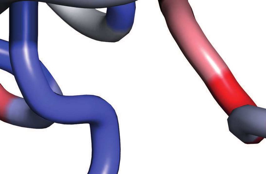
35

                                               Residue ID (end of a segment)
                                                                                                        min GLN =- 0.6
                                                                                                        max GLN = 0.8
                                                                               40

                                                                               45

                                                                               50

                                                                               55

                                                                               60

                                                                               65
                                                                                    35 40      45 50       55 60 65
                                                                                     Residue ID (beginning of a segment)

Figure 1: Left panel: An example of a lasso configuration of L2 type, with
a disulfide bridge (in orange) closing a covalent loop, and a minimal surface
(in gray) which spans the loop and is pierced twice by the tail. Middle
panel: A cartoon representation of a hydrolase protein (PDB code 5uiw,
chain B), with disulfide bridge between amino acids 10 and 34. It is of L2
type, with minimal surface (in gray) and tails coloured according to the GLN
values between their segments and whole loop. Right panel: The topological
fingerprint of a lasso based on the GLN matrix for the same protein. Each
cell of the matrix corresponds to the GLN value between the disulfide loop
and the specific subchain of the tail (here C terminus, the longer one), where
the id of the first residue is on the x-axis and the id of the last residue is on
the y-axis, thus the left bottom corner corresponds to the whole tail. The
C-tail in the middle panel is colored according to the diagonal of the matrix.

sided lasso LL (when a loop is pierced by both tails). It is important to note
that from mathematical point of view all classes of lassos are topologically
equivalent to trivial lasso L0 because the free ends are not prevented from
unwinding. And even if we connected free ends not disturbing windings,
except lasso supercoil LS the rest would be still topologically equivalent to
trivial lasso. But, from biological point of view, they are still very interest-
ing complex structures. For example, a correlation between a type of lasso
topology and the specific function of protein has been identified [11]. All
proteins that form any type of lasso are collected in the LassoProt database
[12].
    Proteins with lassos are found in all domains of life and possess diverse
functions [11, 12]. Lasso topology can influence thermodynamics properties
and biological activity of proteins [13, 14]. Cystein bridges provide stability
to protein structures and a non-trivial topology can enhance this influence
[7, 15]. However, it is also known that non-trivial topology hinders the fold-

                                       3
ing pathway [16], leading to possible misfolding [17]. How evolution solves
this delicate balance is one of the open questions. There are many others
at the interface of biology and mathematics. What is the role of the lasso?
Is there a correlation between the lasso type and the biological function?
How do these proteins fold in oxidative conditions? The latter question
however does not concern the lasso peptides which are class of ribosomally
synthesized posttranslationally modified natural products found in bacteria.
However these peptides have a diverse set of pharmacologically relevant ac-
tivities, including inhibition of bacterial growth, receptor antagonism, and
enzyme inhibition [18]. Thus, can lasso topology be useful in bioengineering
or in pharmacological applications to design proteins with desired fold, sta-
bility or other features? In polymer chemistry, lassos (known as tadpoles)
are used to design materials with desired properties [19, 20, 21]. Since las-
sos are defined using open curves they are also inspiring mathematicians to
construct topological tools capable of classifying them [22, 23]. However, up
to now, the question of whether a loop and a tail can be entangled in protein
while the minimal surface spanned on the loop is not pierced, hasn’t been
asked. How might this entanglement influence protein biophysical proper-
ties? The Gauss linking integral approach could reveal more information
about lasso proteins than the previous geometric method.
    The aim of this research is to better understand the entanglement of
lasso proteins and its influence on their thermodynamical properties. To do
so we first introduce a new technique based on the Gauss linking integral
and, then, apply it to assess the topological complexity of proteins with
disulfide bridges. We show that GLN provides new information about the
entanglement of the loop and tails, related to geometric features of the
minimal disc piercings but, in addition, identifies entangled proteins with
different complex lasso topology. We introduce GLN fingerprint to display
the local winding of a protein backbone and as another method to quantify
entanglement in proteins with non-trivial linking topology. Finally, we use
GLN as descriptor to study the free energy landscape of proteins and show
influence of non-trivial topology on proteins stability and folding pathway.

Results
Our new approach relies on the definition of the Guass linking integral.
Let us first consider a protein chain with a disulfide bond connecting two
amino acids that, in this way, creates an unknotted covalent loop. The
complementary parts of the chain are the tails. When at least one tail

                                     4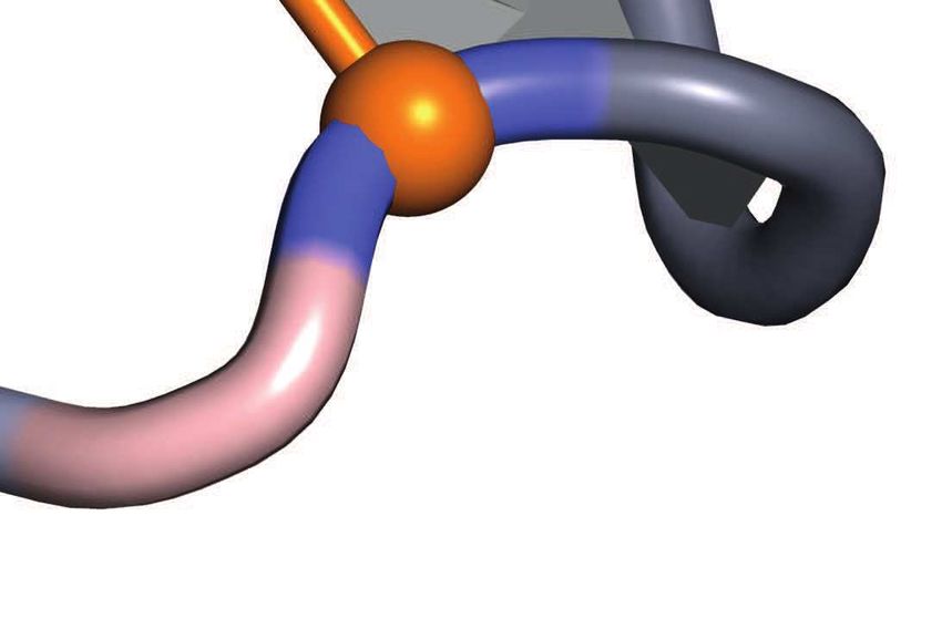
pierces a minimal surface spanned on the loop, the entire structure is called a
complex lasso (Fig. 1). In this study, we compute the Gauss linking integral,
which we denote by GLN, quantifying the linking between each tail and the
closed loop. The GLN is an algebraic measure of how many times (and
in which direction) the tail winds around the loop, with cancellation. For
example, a value of GLN close to 1 means that the tail winds around the
loop more or less once, in total. In the most simple cases, the tail passes once
through the surface spanned on the loop (in a positive direction, following
natural orientation of protein from the N terminus to C terminus). Such
structure resembles the single lasso called L1 . If the direction is reversed, the
linking number is close to −1. Note that, in complex cases, the tail can pass
around the loop twice in a positive direction and once in a negative direction
for an algebraic total of about 1. Moreover, by definition, the linking number
of two unlinked curves is 0 although one can not infer with certainty that
linking number 0 curves can be separated. This is demonstrated by the
“Whitehead” link in which the algebraic linking of the two closed loops is
zero but they are geometrically entangled and one chain intersects a minimal
surface spanned on the other chain at least twice in opposite and therefore
cancelling directions. We will present conditions to identify and classify
proteins with cystein bridges.

GLN definition from protein perspective
The mathematical definition of linking number between two closed curves in
3 dimensions is given by the Gauss double integral. In the case of proteins,
the molecular chains become collections of points, i.e., positions of Cα atoms,
and the integrals may be replaced by sums of exact quantities determined
by pairs of segments connecting the points as determined by the molecular
chain [24]. We must relax the expectation of having an integer indicator of
linking as we perform the double Gauss integral over open chains. See the
section Materials and Methods for the details. We propose the analysis of
four main values for each pair consisting of a loop and a tail:
1) whGLN : the GLN value of a loop and a whole tail,
2) minGLN , and
3) maxGLN
respectively, the minimum and maximum values of GLN between a loop and
any fragment of a tail, and
4) max|GLN | = max{maxGLN, −minGLN }.
Additionally, for each triple of a loop and two tails, we consider max2|GLN |

                                        5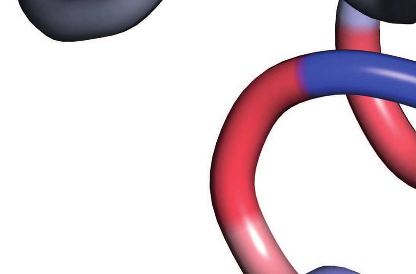
value defined to be the maximum of max|GLN | values for both tails. We
determine the positive directions of windings according to natural direction
of a protein chain; oriented from the N -terminus to the C-terminus. A high
maxGLN or low minGLN indicate that the corresponding part of a tail
significantly winds around a loop in a ”positive” or ”negative” direction,
respectively. Usually the minimal surface spanned on the loop is pierced by
this part of the tail.
    We analyzed the entire set of all 5,106 non-redundant proteins in the
Protein Data Bank with at least one disulfide bridge (13,320 covalent loops
in a total) from the LassoProt database [12]. See Materials and Methods
section for the details about the dataset.
    Application of GLN to this dataset reveals the gaussian distribution with
long tail as shown in Fig. 2. In the majority of cases, the GLN is near 0.2
indicating proteins in which t the minimal surface spanned on the loop is
probably not pierced. However, the long tail shows that, in high fraction
of chains with cysteine bridges at least one tail significantly winds around
the loop. For example, in 21% of chains, we have at least one loop with
max2|GLN | > 0.6 and, in 9.4% of loops, we have max2|GLN | > 0.6. The
value 0.6 seems to be a good threshold with which to distinguish between
complex and trivial topologies, since over 93% of loops with max2|GLN | >
0.6 have the minimal surface spanned on the loop pierced by a tail at least
once and only 4% of loops with max2|GLN | ≤ 0.6 have loop spanning
surfaces pierced by either tail.

The GLN fingerprint as a method to classify lasso structures
To identify the correlation between topology and geometry of proteins, we
adopt the idea of topological fingerprint used to exhibit the internal knots
in proteins called slipknots [6, 25]. Here, we present the linking complexity
in the form of a matrix diagram – for a pair of a loop and a tail – that shows
the GLN between the loop and the entire tail and each of its subchains.

    The analysis of our dataset reveals that covalent loops in proteins can
be classified into a few distinct motifs, represented by particular patterns
within the matrix diagrams. Four characteristic motifs are shown in Fig. 3.
Each point of the matrix corresponds to a specific subchain of the tail, where
the id of the first residue is on the x-axis and the id of the last residue is
on the y-axis. As a consequence, the left bottom corner corresponds to the
whole tail. The color intensity indicates the value of the GLN between the
disulfide loop and the specific subchain of the tail. A red color indicates

                                      6
1

                              0.8

                          0.6

                   Fraction
                              0.4

                          0.2

                    0.094
                              0
                                    0   0.2   0.4   0.6   0.8   1.0   1.2   1.4
                                                    max2|GLN|

Figure 2: The histogram of max2|GLN | values for all closed loops (created
by a disulfide bridge) in the set of 5106 non-redudant proteins. The dotted
curve shows the fraction of loops having max2|GLN | greater than the value
on the x-axis. Almost 10% of the loops have max2|GLN | greater than 0.6
indicating significant entanglement with a tail. Schematic figures show the
most probable corresponding type of the lasso structure.

negative linking values reflecting the negative direction while blue indicates
positive linking values. These GLN matrices are used to introduce the fol-
lowing classification of proteins with cystein bridges:
• gL0 , no clear colorfull patches in the matrix indicating that the tail does
not wind around the loop.
• gL1 , there is one colorfull patch in the matrix (e.g. in the left bottom
corner) indicating that the tail winds around the loop once. The color indi-
cates the direction.
• gL2 , there are two patches in different colors in the matrix, (e.g. one
on the left edge and second one on the bottom edge). This indicates that
the tail winds around the loop in one direction and then in the opposite
direction. (This spatial arrangement can be observed by following the left
edge of the matrix in a descending direction: the beginning of the analyzed
segment remains the same - beginning of the tail - while the end of the ana-
lyzed segment is moving towards the end of the tail. When we approach the
patch, a color begins to appear meaning the tail begins to wind around the
loop. Below the colorfull patch we again see white indicating that the tail
winds around the loop but in the opposite direction thereby cancelling the
initial winding contribution. Thus the windings ”cancel” themselves and
the corner of matrix is again almost white (see Fig. 1).).

                                                      7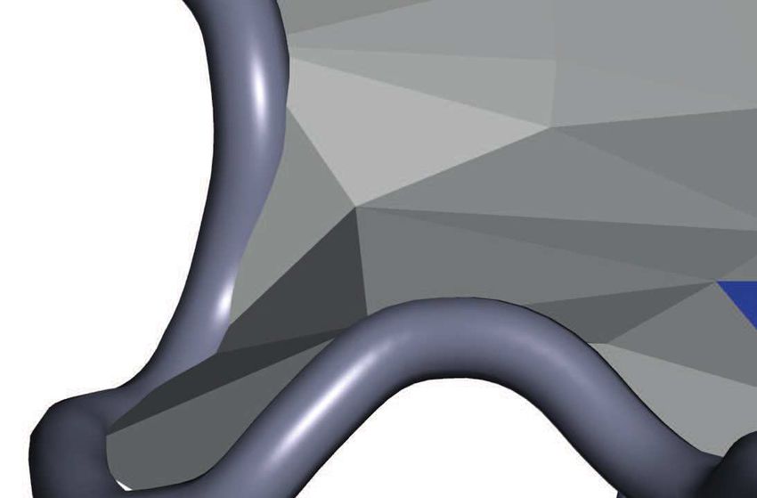
• gL3 , there are four colorfull patches in the matrix, e.g. one in the middle
in the different color than three other patches; this indicates that the tail
winds around the loop in one direction, then turns and winds around the
loop in the opposite direction, and finally turns back one more time.
• gLn , for any natural n, there  is specific, dependent on n, number of col-
                          n+1
                                n+2
orfull patches (namely 2 · 2 ) in the matrix; this indicates that tail
winds around the loop n times, each next time in the opposite direction.
• gLS, there is usually one big patch in one color which at some point be-
comes very intensive - claret or navy in the case of negative and positive
windings, respectively; this means that the tail winds around the loop in
one direction (making a full circle) and then winds around it one more time
in the same direction.
• gLL, if both matrices for two tails have at least one colorfull patch; this
indicates that both tails wind around the loop.

    Similar GLN matrices indicate the same topological motifs even though
the chains may have a different structure. Examples of the same GLN
matrices for proteins with very low sequence similarity are shown in Sup-
plementary Information (Fig. 4 and Fig. 5). The motifs gLn , gLS and gLL
usually correspond to the lasso types Ln , LS and LL, respectively. The GLN
matrices reveal much more detail about the geometry of the chains with las-
sos. By analysing the location, size and color of a collection of patches one
may deduce which parts of the tail wind around the loop and how fast and
tightly they wind. For the most part intense patches correspond to the tail
piercing the minimal surface spanned on the loop. This is not always the
case since the tail may make almost full circle around the loop, but do not
pierce the minimal surface spanned on the loop (see Table 1). Such complex
configurations had not been identified by methods that studied intersetions
with the minimal surface spanned on the loop [11].

Classification of lasso protein structures and entangled but
unpierced loops
In this section we describe some methods to classify proteins with lassos
based on the Gauss linking integral. We propose a precise classification of
loop-tail pairs having distinct linking motifs presented by the GLN finger-
prints (Fig. 3). This is based on three positive real numbers tL , tL+ , tLS (for
instance tL , tL+ ≈ 0.6, tLS ≈ 1.5), as follows:
• gL0 - if max|GLN | ≤ tL , • gLS - if max|GLN | > tLS ;
In the all next three cases we demand that max|GLN | ∈ (tL , tLS ], and:

                                       8
Figure 3: Topological fingerprints – GLN matrices. Left, the fingerprints
gL1 (top) and gL3 (bottom), respectively, for proteins with one and three
piercings of the , based on proteins with pdb codes 1i1j and 2ehg. Right, the
fingerprints gL2 (top) and gLS (bottom), respectively, for proteins with two
piercings of the minimal surface spanned on the loop in the opposite direction
and the same direction (supercoiling), based on proteins with pdb codes 2ehg
and 1zd0. Arrows begin in the places on the matrices where color is rapidly
changing implying that the tail is in the critical phase of winding around
the loop and the GLN is quickly increasing or decreasing. On the other side,
on the diagrams they indicate the neighborhoods of possible corresponding
piercings. The colors of the arrows indicate directions of windings.

                                      9
Minimal surface classiifiication                   GLN classification
                      0                                         0

                    -0.5                                      -0.5

                    -1.0
           axGLN

                                                              -1.0
          min GLN

                    -1.5                                      -1.5
                                                 L0                                         gL 0
                                                 L1+                                        gL 1+
                    -2.0                         L2+          -2.0                          gL 2+
                                                 L 3+                                       gL 3+
                                                 LS                                         gLS
                    -2.5                                      -2.5
                           0   0.5   1.0   1.5   2.0    2.5          0    0.5   1.0   1.5    2.0    2.5
                                      max GLN                                   max GLN

Figure 4: Classification of proteins with closed covalent loop based on the
minimal surface technique (left) and GLN technique (right). As much as
98% of structures are classified in an analogous way by both techniques
(corresponding points are colored in the same way on both plots). However,
on the right, plot types are divided more regularly since the corresponding
classification is based only on the GLN values. To differenciate between the
types gL2+ and gL3+ on the plots (green and red dots, respectively) one
needs the third coordinate - whGLN value.

• gL1 - if exactly one value of maxGLN and −minGLN is greater than tL ,
• gL2+ - if both values maxGLN and −minGLN are greater than tL and
|whGLN | ≤ tL+ ,
• gL3+ - if both values maxGLN and −minGLN are greater than tL and
|whGLN | > tL+ .
One can consider whole triple consisting of a loop and two tails: if one of
the tails is classified as gL0 , then we say that the triple is of the type of the
second tail; if both tails are classified in different way than gL0 , we say that
the triple is of the type gLL.
    Let L2+ denote the sum of types L2n for any natural n ≥ 1 (in proteins
we have found so far examples of L2 , L4 and L6 , see [12]). Let L3+ denote
the sum of types L2n+1 for any natural n ≥ 1 (in proteins we only know
examples of L3 ). We found that it is possible to choose particular values
of tL , tL+ , tLS (i.e. tL = 0.69, tL+ = 0.6, tLS = 1.55) such that as much as
98% of loops are classified in an analogous way by both the techniques of
minimal surfaces and the GLN as shown in the Fig. 4 (see Supplementary
Information Fig. 5 for detailed comparison). Most of the remaining 2%
of loops are structures with intriguing properties that were not recognized

                                                        10
before [11]. We split them into the three groups.
The first group consists of proteins in which the minimal surface spanned
on the loops are not pierced but the tails strongly wind around the loop, or
the surfaces spanned on loops are twisted and wind around the tails. When
the loop is twisted it appears that there is not enough space to thread the
tail through the loop although it is composed of more than 100 amino acids.
There are only 15 such proteins among the set of non-redundant chains of a
length lower than 500 amino acids (see Table 1), with max|GLN | > 0.69 and
no piercings. One can ask how does this type of entanglement influence the
free energy landscape of the protein in oxidizing conditions? We speculate
that, in this case, some part of the configurational space is excluded from
protein backbone exploration during folding. Unwanted threading will have
to backtrack thereby slowing down folding or even leading to missfolding.
The second group contains proteins with high |GLN | values and the
closed loops that are pierced by the tails, but, in minimal surface technique,
these piercings are interpreted as being too shallow and are reduced, i.e.
they are not taken into account. (Generally, this is a reasonable approach
since, for instance, all helices that are crossing surfaces usually do cross them
at least three times on a short distance. We wish to interpret this as simply
one meaningful crossing. However, it is not an easy problem to distinguish
shallow crossings from relevant ones (see Supplementary Information Fig. 6)
and the parallel analysis of GLN matrices may be very helpful in recognizing
which reductions are justified or are spatially reasonable.)
The third group consists of structures with low max|GLN | value but
with tails piercing the minimal surface spanned on the loops. There are only
9 such loops (0.01% of the analyzed data set), see Supplementary Informa-
tion, Table 1. (These structures have max|GLN | ≤ 0.6 and no examples
with max|GLN | < 0.5 (see Table 1 in Supplementary Information). With
a detailed analysis, we found that in some structures the GLN value is low
because the piercing segment lies in the plane of the loop - i.e. is quite
”shallow”.)
Unique biophysical features of lasso proteins
An analysis of the statistics concerning GLN reveals interesting features
from the biological point of view. First of all, the windings in the negative
direction occur significantly more often than those in the positive direction.
For example, among the loops of gL1 type over 63% have a negative GLN
value (see Fig. 5, panel B). However, a detailed analysis of basic physico-
chemical properties (a type of amino acids, type of disulfide bridge [26]) does
11Table 1: “Entangled“ proteins without piercing through a covalent loop
closed by a disulfide bridge. Based on loops from non-redundant chains
of a length lower than 500 amino acids, which are not pierced, but have
max|GLN | > 0.69.
Protein Loop
Tail Max|GLN|
(chain) range
2bb6 (A) 98-294 N 0.99
1ece (A) 34-120 N 0.91
4e9i (C) 53-135 C 0.87
4df0 (A) 148-198 N 0.83
3vv5 (A) 97-235 N (-) 0.79
2pmv (A) 85-270 N 0.78
4m82 (A) 275-397 N 0.78
1uhg (A) 73-120 C 0.77
4wtp (A) 218-264 N 0.76
2b34 (A) 20-114 N 0.74
2x5x (A) 36-85 C 0.74
5acf (A) 41-167 C 0.73
1qfx (A) 52-368 C (-) 0.72
5fzp (A) 12-72 C (-) 0.72
2dw2 (A) 308-388 N 0.70
yet not provide an explanation of this difference.
The histogram of all whGLN values reveals a noticeable depression
around the value −0.5 (see Fig. 5, panel C). This shows that there are
only a few tails that come close to the loop but are not pierced through it.
In the case of the random polymers with the same size of the loop and tails,
such behaviour is not observed (see Fig. 5, panel D). This implies that the
depression in proteins distribution arises from a specific side chain interac-
tion which makes contacts outside the loop or, if they are close enough, to
the loop whose the minimal surface spanned on the loop they would pierce.
Considering the lengths of loops and tails we find that the average value
of maxGLN depends logarithmically on the length of a tail, up to a length
of around 40 amino acids. Next, maxGLN saturates and remains stable
around the value 0.25 (0.55 for polymers) (see Fig. 6).
Finally, the analysis of B-factors (the temperature factor) shows that
123000 90 5000 random
}
polymers
2500
70 4000
2000
3000
50
1500
2000
1000 40
500 1000
40
0 0
-2 -1 0 1 2 -1.5 -1 -0.5 0 0.5 1 1.5 -2 -1 0 1 2 -2 -1 0 1 2
min GLN max GLN min GLN max GLN wh GLN wh GLN
Figure 5: Distribution of maxGLN , minGLN and whGLN values based
on the 13,320 loops closed by disulfide bridges. Panels A,B,C indicate that
there are more negative GLN values than positive ones in proteins. A)
Histogram of all maxGLN and minGLN values that are greater than 0.15
or lower than −0.15, and 53% of them are negative. B) Histogram of all
maxGLN or minGLN values (only greater value - in the sense of absolute
value - from each pair is taken into account here) from the loops of gL1 type
- over 63% of them are negative. C) Histogram of all whGLN values in the
analyzed dataset revealing the local minimum around the value −0.5. D)
Histogram of whGLN for random polymers.
0.7
0.7 0.7
0.7 0.7
0.7
Fit t ed funct ion (log) Fit t ed funct ion ( log) Dat a - Lasso Prot eins
Dat a Dat a Random Polim ers
0.6
0.6 0.6
0.6 0.6
0.6
Average max|GLN|
0.5
0.5 0.5
0.5 0.5
0.5
Average m ax|GLN|
0.4
0.4 0.4
0.4 0.4
0.4
0.0.3
3 0.0.3
3 0.0.3
3
0.2
0.2 0.2
0.2 0.2
0.2
0.1
0.1 0.1
0.1 0.1
0.1
0.0
0.0 0.0
0.0 0.0
0.0
− 20
00 20 40 60 80 100 120
40 80
N t ai engt h
120 140 160 − 20 0
0
20 40 60
40C t ai 80
80 100 120 140 160
engt h
120
− 20
00 20 40 60 80 100 120
40 80
Tai engt h
120 140 160
N tail length C tail length Tail length
Figure 6: Left and middle panels: average max|GLN | values for different
lengths of N and C-tails, respectively - first they grow logarithmically, then
they become more or less constant, equal to about 0.25. Right panel: com-
parison of average max|GLN | values for different lengths of tails in proteins
(N and C-tails counted together) and for random polymers. The plot reveals
a similar pattern but with much higher GLN values in polymers, stabilizing
around 0.55.
13in chains with short loops amino acids for which |GLN | between the loop
and the tail’s fragment from begining to the amino acid is the highest, have
higher B-factors than average ones. Moreover, amino acids for which |GLN |
between the loop and the unit segment corresponding to the amino acid is
the highest (often those segments pierce the minimal surface spanned on
the loop) – have significantly lower B-factors, lower even than amino acids
creating cysteine bridges. For all loops the tendency is similar, however
a little bit less strong (see Table 2). This suggests that the parts of tails
piercing the loops spanning surfaces are more stable, while the parts of tails
between bridges and crossings fluctuate more. This is in agreement with
available experimental data for lasso type polypetides [27].
Table 2: Correlation between GLN values (of unit segments of tails and
whole loop) and B-factors for corresponding amino acids in lasso proteins.
Second column: proteins with loops consisting of less than 50 amino acids
are taken into account. Third column: all loops.
Average B-factor for amino acids – Short loops All loops
all < amino acids > 31.0 28.3
creating bridges 29.7 28.4
for which GLN between the loop
and the tail’s fragment from 34.2 30.7
beginning to them is the highest
for which GLN between the loop
26.4 23.7
and the unit segment is the highest
The strong correlation between GLN values of unit segments and whole
loop, and B-factors for corresponding amino acids is clearly visible in Fig. 7.
High B-factors correlate with low |GLN | values and inversely - high |GLN |
values correlate with low B-factors. This again suggests that pieces of the
tail winding around the loop are more stable that the other segments of the
tail.
Applications of the GLN fingerprint
Understanding the mechanism by which proteins fold to their native struc-
ture is a central problem in protein science [28]. In the case of a majority
of proteins, native contacts are sufficient to drive the folding of the protein
1430
Residue ID (end of a segment) 10
40 low |GLN|
high B-factor
low |GLN| 20
50
high B-factor
60 30
70 40
80 50
30 40 50 60 70 80 10 20 30 40 50
Residue ID (begining of a segment) Residue ID (begining of a segment)
Figure 7: Correlation between GLN values and B-factors shown in the GLN
matrices for proteins (left: pdb id 4ors, with the loop closed by amino
acids 89-186, right: pdb id 2ehg, with the loop 58-145; matrices are for
N-terminals), both of gL3 type. On the right edge of the matrix, B-factors
are in black and |GLN | values between unit segments and whole loop are in
green. Note that when a local |GLN | is high it usually means that the tail
is just winding around the loop, which results in color changes on the left
edge of the matrix. When local |GLN | is low, the tail is often far from the
loop, not winding around it as significantly at that location.
[29, 30, 31] since their free energy landscape is minimally frustrated [32].
The fraction of native contacts, called Q, was shown to be a good reaction
coordinate to study the folding mechanism for a majority of proteins [28].
However, in the case of proteins with non-trivial topology (e.g. the smallest
knotted protein MJ0366 [33]), Q merely represents the progress of folding
[34].
Next, we show that the GLN values and the GLN fingerprint can reveal
information, hidden from Q, about the topology based on unfolding path-
ways simulated with a structure based model [35]. In fact, in the case of
the ribonuclease U2 protein with the gL3 motif (the loop is pierced three
times), GLN values reveal an ensemble of the transition states composed
of at least two unfolding pathways: via the slipknot topology [16, 36] or
direct unthreading (see Fig. 8). Moreover, superposition of the fingerprints
over the time shows how the protein backbone travels through the available
conformation space. The same technique can be applied to reveal untying
of even more complex topologies such as the supercoling motif gLS (one
tail winding around the loop and piercing it two or more times from the
same site). The unfolding pathway for a protein with gLS3 is shown in
Supplementary Information Fig. 7.
15Native
Pathway I
protein Pathway II
gL 3
gL3 gL 1 gL 3 gL 2 gL 0
gL 0
Residue ID (end of a segment)
60 60
60
70 70 70
80 80 80
90 90 90
100 100 100
110 110 110
60 70 80 90 100 110 140 150 160 170 290 320 340 360
Residue ID
(begining of a segment) Time Time
Figure 8: Example of two topologically different unfolding routes identified
with GLN method for the ribonuclease U2 (pdb ID 3agn) with gL3 motif
(the closed loop is pierced three times). Left panel: the GLN matrix at
the native conformation. Middle panel: visualization of unfolding via un-
threading internal loop toward gL1 motif, next single unthreading to trivial
topology. Each column of this matrix corresponds to the single time frame
in the simulation and represents left edge of the GLN matrix for this frame.
Right panel: untying to gL2 geometry, next untying via slipknot motif to
gL0 .
16The application of the GLN is not limited to studying lasso proteins or
proteins with links [7]. Since the GLN measures mutual entanglement its fin-
gerprint is different for “the same“ protein with two topologies – unknotted
and knotted (see Supplementary Information Fig. 8) [37]. Furthermore, the
pattern of the GLN fingerprint can be used to identify the type of secondary
structures of the protein which are usually visible via a contact map. Note,
that the shape of the contact map depends on the cutoff distance used to
determine physical contacts while GLN does not depend on additional pa-
rameters. Moreover, sign of GLN (blue or red color on the matrix) indicates
the ”direction of contact”, i.e. from this it can be deduced on which side the
fragments of protein chain being in contact pass each other (for more details
see Supplementary Information Fig. 8, Fig. 9). Thus, the GLN fingerprint
of a native conformation can be used as a reference value for a reaction
coordinate in studying the folding pathways of protein.
Discussion and conclusions
We have shown that the GLN method is a significantly faster technique to
detect entanglement in proteins with closed loops in the comparison with
the methods which rely on minimal surfaces spanning the covalent loops
[11]. The method also reveals much more information about the geometry
of chains with lassos which may lead to the new biological and chemical
discoveries. However, the algorithm based on the surfaces has the advantage
of giving precise information about the exact residues that cross the spanning
surface which may lead to an important insight from the biological point of
view. We believe both approaches can compliment each other and, together,
help focus study on important features of the protein.
The GLN fingerprint can also be used to compare proteins e.g. during
CASP or CAPRI competition. Indeed, it can be pushed further, so that the
GLN fingerprint provides a powerful tool to be used to improve already very
successful deep learning algorithms used to predict tertiary and quaternary
structure of proteins via image recognition [38].
The present method can be applied to any structure in which a loop and
tail can be defined. Apart from the cysteine bridge loops investigated here, a
loop can be formed, among others, by a salt bridge, by a hydrogen bond, or
by ions. An example of the last case is the human transport protein (PDB
code 1n84), with the loop closed by Tyr95-Fe339-Asp63 interaction whose
spanning surface is pierced by C-terminal tail (Thr250) [39] thus forming
lasso of gL1 type.
17Moreover, one can apply GLN approach to study entanglement be-
tween two structures none of which are closed loops. Lately new algorithm,
GISA, was proposed to study local entanglement in protein chains and other
biopolymers [40]. The algorithm computes Gauss integrals between many
pairs of quite short fragments of chain and finds rare invariant values. It
can be helpful in search for knots, links and highly entangled configurations
not previously described as well. Furthermore since this approach is much
faster than other linking invariants it will provide a very useful technique to
study loops in a single chromosome as well as chromosome entanglement in
the cell [41, 42]. Current methods allow one to describe single chromosomes
with high resolution (thousands of beads). This number is already an order
of magnitude bigger than the typical length of the protein.
Materials and Methods
Gaussian linking number. A definition of linking number between two
closed curves γ1 and γ2 in 3 dimensions is given by the Gauss double integral,
~r(1) − ~r(2)
I I
1
GLN ≡ · (d~r(1) × d~r(2) ), (1)
4π γ1 γ2 |~r(1) − ~r(2) |3
where ~r(1) and ~r(2) are positions of two curves. Gauss proved that, for closed
oriented curves, this integral is always integer, is an invariant up to isotopy,
and measures how many times one curve winds around the second one. In
the protein case chains become collections of points, i.e., positions of Cα
(k) (k) (k)
atoms {~r1 , ~r2 , . . . ~rNk }, for the chains of the length Nk , k = 1, 2. The
integrals may be replaced by sums over segments dR ~ (k) = ~r(k) − r~i (k) , for
i i+1
which we use the midpoint approximation R ~ (k) = (~r(k) + r~i (k) )/2. We can
i i+1
replace the requirement of having oriented closed loops by oriented open
arcs giving a real value as a measure of linking rather than an integer. We
can then perform the double Gauss discrete integral over the open chains,
N1 −1 NX
1 X 2 −1 ~ (1) − R
R ~ (2)
i j ~ (1) × dR
~ (2) ).
GLN ≡ (1) (2) 3
· (dR i j (2)
4π ~ ~
i=1 j=1 |R −R | i j
Note, one can simply employ the Banchoff method on the open
chain to explicitly calculate this integral [24].
18Let us denote
~ (1) − R
R ~ (2)
i j ~ (1) × dR
~ (2) ),
G(i, j) := · (dR i j (3)
~ (1)
|R − ~ (2) |3
R
i j
i ∈ {1 . . . N1 − 1}, j ∈ {1 . . . N2 − 1}, and consider a pair of a tail of a length
N1 and a loop of a length N2 . We calculate and then analyze four main
values for each pair of a loop and a tail:
• whGLN : value of the Gauss double integral between a loop and whole
tail,
N1 −1 NX
2 −1
1 X
whGLN = G(i, j); (4)
4π
i=1 j=1
• minGLN (maxGLN ): minimum (maximum) value of the Gauss dou-
ble integral between a loop and any fragment of a tail,
l N2 −1
1 X X
minGLN = min G(i, j); (5)
k,l∈{1...N1 −1}, 4π
kPyLink [46] plugin for PyMOL were used to facilitate analysis and perform
Molecular graphics.
Molecular dynamics simulation. The kinetics data were obtained
based on a coarse-grained model and conducted using the Gromacs package
with SMOG software [35] employing parameters from [47].
Random lassos sampling. Phantom lassos (polymers deprived of any
interactions and volume) were created by connecting phantom loops and
phantom tails. Phantom loops were created as equilateral polygons using
the dedicated algorithm [48] and tested earlier in the [49].
Acknowledgments
The authors would like to thank Szymon Niewieczerzal, Bartosz Gren for help with
running simulations, Eleni Panagiotou, Pawel Dabrowski-Tumanski for useful dis-
cussions. This work was financed from the budget of Polish Ministry for Science and
Higher Education Grant [#0003/ID3/2016/64 Ideas Plus] to JIS, and University of
Warsaw [#501-D313-86-0117000-03] to WN.
Author Contribution
J.I.S., K.C.M. and W.N designed the work, W.N. and J.I.S performed the work
and wrote the paper.
Additional information
Supplementary Information is attached. Competing financial interests: The
authors declare no competing financial interests.
References
[1] M. H. Glickman, A. Ciechanover, The ubiquitin-proteasome proteolytic
pathway: destruction for the sake of construction, Physiological reviews
82 (2) (2002) 373–428.
[2] P. Virnau, L. A. Mirny, M. Kardar, Intricate knots in proteins: Function
and evolution, PLoS computational biology 2 (9) (2006) e122.
[3] K. C. Millett, E. J. Rawdon, A. Stasiak, J. I. Sulkowska, Identifying
knots in proteins (2013).
20[4] M. Jamroz, W. Niemyska, E. J. Rawdon, A. Stasiak, K. C. Millett,
P. Sulkowski, J. I. Sulkowska, Knotprot: a database of proteins with
knots and slipknots, Nucleic acids research 43 (D1) (2015) D306–D314.
[5] N. P. King, E. O. Yeates, T. O. Yeates, Identification of rare slipknots
in proteins and their implications for stability and folding, Journal of
molecular biology 373 (1) (2007) 153–166.
[6] J. I. Sulkowska, E. J. Rawdon, K. C. Millett, J. N. Onuchic, A. Stasiak,
Conservation of complex knotting and slipknotting patterns in pro-
teins, Proceedings of the National Academy of Sciences 109 (26) (2012)
E1715–E1723.
[7] P. Dabrowski-Tumanski, J. I. Sulkowska, Topological knots and links
in proteins, Proceedings of the National Academy of Sciences 114 (13)
(2017) 3415–3420.
[8] J. H. White, Self-linking and the gauss integral in higher dimensions,
American Journal of Mathematics 91 (3) (1969) 693–728.
[9] P. Røgen, B. Fain, Automatic classification of protein structure by us-
ing gauss integrals, Proceedings of the National Academy of Sciences
100 (1) (2003) 119–124.
[10] M. Baiesi, E. Orlandini, F. Seno, A. Trovato, Exploring the correlation
between the folding rates of proteins and the entanglement of their
native states, Journal of Physics A: Mathematical and Theoretical.
[11] W. Niemyska, P. Dabrowski-Tumanski, M. Kadlof, E. Haglund,
P. Sulkowski, J. I. Sulkowska, Complex lasso: new entangled motifs
in proteins, Scientific reports 6 (2016) 36895.
[12] P. Dabrowski-Tumanski, W. Niemyska, P. Pasznik, J. I. Sulkowska,
Lassoprot: server to analyze biopolymers with lassos, Nucleic acids
research 44 (W1) (2016) W383–W389.
[13] E. Haglund, J. I. Sulkowska, Z. He, G.-S. Feng, P. A. Jennings, J. N.
Onuchic, The unique cysteine knot regulates the pleotropic hormone
leptin, Plos one 7 (9) (2012) e45654.
[14] E. Haglund, J. I. Sulkowska, J. K. Noel, H. Lammert, J. N. Onuchic,
P. A. Jennings, Pierced lasso bundles are a new class of knot-like motifs,
PLoS computational biology 10 (6) (2014) e1003613.
21[15] S. Niewieczerzal, J. I. Sulkowska, Supercoiling in a protein increases its
stability, Physical review letters 123 (13) (2019) 138102.
[16] J. I. Sulkowska, P. Sulkowski, J. Onuchic, Dodging the crisis of folding
proteins with knots, Proceedings of the National Academy of Sciences
106 (9) (2009) 3119–3124.
[17] M. Qin, W. Wang, D. Thirumalai, Protein folding guides disulfide bond
formation, Proceedings of the National Academy of Sciences 112 (36)
(2015) 11241–11246.
[18] M. O. Maksimov, I. Pelczer, A. J. Link, Precursor-centric genome-
mining approach for lasso peptide discovery, Proceedings of the Na-
tional Academy of Sciences 109 (38) (2012) 15223–15228.
[19] Y. Tezuka, H. Oike, Topological polymer chemistry: systematic classifi-
cation of nonlinear polymer topologies, Journal of the American Chem-
ical Society 123 (47) (2001) 11570–11576.
[20] H. R. Kricheldorf, Cyclic polymers: Synthetic strategies and physi-
cal properties, Journal of Polymer Science Part A: Polymer Chemistry
48 (2) (2010) 251–284.
[21] Y. Tezuka, Topological polymer chemistry designing complex macro-
molecular graph constructions, Accounts of Chemical Research 50 (11)
(2017) 2661–2672.
[22] W. Tian, X. Lei, L. H. Kauffman, J. Liang, A knot polynomial invari-
ant for analysis of topology of rna stems and protein disulfide bonds,
Molecular Based Mathematical Biology 5 (1) (2017) 21–30.
[23] P. Dabrowski-Tumanski, J. I. Sulkowska, The aps-bracket – a topologi-
cal tool to classify lasso proteins, rnas and other tadpole-like structures,
Reactive and Functional Polymers.
[24] T. Banchoff, Self linking numbers of space polygons, Indiana Univ.
Math. J. 25 (12) (1976) 1171–1188.
[25] T. O. Yeates, T. S. Norcross, N. P. King, Knotted and topologically
complex proteins as models for studying folding and stability, Current
opinion in chemical biology 11 (6) (2007) 595–603.
[26] G. Bulaj, Formation of disulfide bonds in proteins and peptides,
Biotechnology advances 23 (1) (2005) 87–92.
22[27] M. Zimmermann, J. D. Hegemann, X. Xie, M. A. Marahiel, The
astexin-1 lasso peptides: biosynthesis, stability, and structural studies,
Chemistry & biology 20 (4) (2013) 558–569.
[28] R. B. Best, G. Hummer, W. A. Eaton, Native contacts determine pro-
tein folding mechanisms in atomistic simulations, Proceedings of the
National Academy of Sciences 110 (44) (2013) 17874–17879.
[29] J. D. Bryngelson, J. N. Onuchic, N. D. Socci, P. G. Wolynes, Funnels,
pathways, and the energy landscape of protein folding: a synthesis,
Proteins: Structure, Function, and Bioinformatics 21 (3) (1995) 167–
195.
[30] P. G. Wolynes, J. N. Onuchic, D. Thirumalai, Navigating the folding
routes, Science 267 (5204) (1995) 1619.
[31] D. Thirumalai, E. P. O’Brien, G. Morrison, C. Hyeon, Theoretical per-
spectives on protein folding, Annual review of biophysics 39 (2010)
159–183.
[32] P. G. Wolynes, Recent successes of the energy landscape theory of pro-
tein folding and function, Quarterly reviews of biophysics 38 (4) (2005)
405–410.
[33] D. Bölinger, J. I. Sulkowska, H.-P. Hsu, L. A. Mirny, M. Kardar, J. N.
Onuchic, P. Virnau, A stevedore’s protein knot, PLoS Comput Biol
6 (4) (2010) e1000731–e1000731.
[34] P. Dabrowski-Tumanski, A. Jarmolinska, J. Sulkowska, Prediction of
the optimal set of contacts to fold the smallest knotted protein, Journal
of Physics: Condensed Matter 27 (35) (2015) 354109.
[35] J. K. Noel, P. C. Whitford, K. Y. Sanbonmatsu, J. N. Onuchic, Smog@
ctbp: simplified deployment of structure-based models in gromacs, Nu-
cleic acids research 38 (suppl 2) (2010) W657–W661.
[36] J. K. Noel, J. I. Sulkowska, J. N. Onuchic, Slipknotting upon native-
like loop formation in a trefoil knot protein, Proceedings of the National
Academy of Sciences 107 (35) (2010) 15403–15408.
[37] The protein from si (pdb id 1oy5) was crystallized as unknotted, how-
ever, it is expected that it is knotted since it was shown that the knotted
topology is strictly conserved for homologous proteins [6], the knotted
23homological protein (pdb id 4yqd) was used to model the knotted ver-
sion of this protein.
[38] M. Gao, H. Zhou, J. Skolnick, Destini: A deep-learning approach
to contact-driven protein structure prediction, Scientific reports 9 (1)
(2019) 1–13.
[39] P. Dabrowski-Tumanski, Knots, lassos and links, topological manifolds
in biological objects, Thesis (2018) 1–150.
[40] C. Grønbæk, T. Hamelryck, P. Røgen, Gisa: Using gauss integrals
to identify rare conformations in protein structures, bioRxiv (2019)
758029.
[41] J. I. Sulkowska, S. Niewieczerzal, A. I. Jarmolinska, J. T. Siebert,
P. Virnau, W. Niemyska, Knotgenome: a server to analyze entangle-
ments of chromosomes, Nucleic acids research 46 (W1) (2018) W17–
W24.
[42] S. Niewieczerzal, W. Niemyska, J. I. Sulkowska, Defining and detecting
links in chromosomes, Scientific reports 9 (1) (2019) 1–10.
[43] A. I. Jarmolinska, M. Kadlof, P. Dabrowski-Tumanski, J. I. Sulkowska,
Gaprepairer: a server to model a structural gap and validate it using
topological analysis, Bioinformatics 34 (19) (2018) 3300–3307.
[44] B. Webb, A. Sali, Protein structure modeling with modeller, Protein
Structure Prediction (2014) 1–15.
[45] A. M. Gierut, W. Niemyska, P. Dabrowski-Tumanski, P. Sulkowski, J. I.
Sulkowska, Pylasso: a pymol plugin to identify lassos, Bioinformatics
33 (23) (2017) 3819–3821.
[46] A. Gierut, P. Dabrowski-Tumanski, W. Niemyska, K. C. Millett, J. I.
Sulkowska, Pylink: a pymol plugin to identify links, under review.
[47] J. I. Sulkowska, M. Cieplak, Selection of optimal variants of gō-like
models of proteins through studies of stretching, Biophysical journal
95 (7) (2008) 3174–3191.
[48] J. Cantarella, B. Duplantier, C. Shonkwiler, E. Uehara, A fast direct
sampling algorithm for equilateral closed polygons, Journal of Physics
A: Mathematical and Theoretical 49 (27) (2016) 275202.
24[49] P. Dabrowski-Tumanski, B. Gren, J. I. Sulkowska, Statistical proper-
ties of lasso-shape polymers and their implications for complex lasso
proteins function, Polymers 11 (4) (2019) 707.
25You can also read