Impact of double-diffusive convection and motile gyrotactic microorganisms on magnetohydrodynamics bioconvection tangent hyperbolic nanofluid
←
→
Page content transcription
If your browser does not render page correctly, please read the page content below
Open Physics 2020; 18: 74–88
Review Article
Tanveer Sajid*, Muhammad Sagheer, Shafqat Hussain, and Faisal Shahzad
Impact of double-diffusive convection and motile gyrotactic
microorganisms on magnetohydrodynamics bioconvection
tangent hyperbolic nanofluid
https://doi.org/10.1515/phys-2020-0009 to be explored widely because of its enormous applications in
received July 07, 2019; accepted February 10, 2020 the field of pharmaceutical industry, purification of cultures,
Abstract: The double-diffusive tangent hyperbolic nanofluid microfluidic devices, mass transport enhancement and
containing motile gyrotactic microorganisms and magneto- mixing, microbial enhanced oil recovery and enzyme
hydrodynamics past a stretching sheet is examined. By biosensors. Bioconvection systems could be categorized
adopting the scaling group of transformation, the governing based on the directional motion of different species of
equations of motion are transformed into a system of microorganisms. In particular, gyrotactic microorganisms are
nonlinear ordinary differential equations. The Keller box the ones whose swimming direction is dependent on a
scheme, a finite difference method, has been employed for the balance between gravitational and viscous torques [4,5].
solution of the nonlinear ordinary differential equations. The Oyelakin et al. [6] pondered the impact of bioconvection and
behaviour of the working fluid against various parameters of motile gyrotactic microorganisms on the Casson nanofluid
physical nature has been analyzed through graphs and tables. past a stretching sheet and observed that the microorganism
The behaviour of different physical quantities of interest profile decreases as a result of an increment in the Peclet
such as heat transfer rate, density of the motile gyrotactic number. Saini and Sharma [7] explored the effects of
microorganisms and mass transfer rate is also discussed in the bioconvection and gyrotactic microorganisms on the nano-
form of tables and graphs. It is found that the modified Dufour fluid flow over a porous stretching sheet. It is noted that
parameter has an increasing effect on the temperature profile. the Lewis number escalates the bioconvection process.
The solute profile is observed to decay as a result of an Dhanai et al. [8] explored the impact of bioconvection on
augmentation in the nanofluid Lewis number. the fluid flow over an inclined stretching sheet and assessed
that the microorganism density profile is enhanced with
Keywords: magnetohydrodynamics, bioconvection, an improvement in the bioconvection Schmidt number.
gyrotactic microorganisms, nanofluid, magnetic field, Mahdy [9] pondered the effects of motile microorganisms
Keller box method, stretching sheet, double diffusion on the fluid past a stretching wedge and noted that a positive
variation in the Peclet number leads to an augmentation in
the microorganism profile. Avinash et al. [10] pondered the
1 Introduction impact of bioconvection and aligned magnetic field on the
nanofluid flow over a vertical plate and concluded that
In fluid dynamics, bioconvection [1–3] occurs when
the heat transfer rate increases with an improvement in the
microorganisms, which are denser than water, swim
Lewis number. Makinde and Animasaun [11] studied the
upwards. The upper surface of the fluid becomes thicker
effects of magnetohydrodynamics (MHD), bioconvection,
due to the assemblage of microorganisms. As a result, the
nonlinear thermal radiation and nanoparticles on fluid past
upper surface becomes unstable and microorganisms fall
an upper horizontal surface of a paraboloid of revolution and
down, which creates bioconvection. Bioconvection continues
found that the Brownian motion boosts the concentration
profile. Khan et al. [12] studied the impact of MHD, gyrotactic
* Corresponding author: Tanveer Sajid, Capital University of Science microorganisms, slip condition and nanoparticles on the fluid
and Technology (CUST), Islamabad, Pakistan, e-mail: tanveer.sajid15@ flow over a vertical stretching plate; it was observed that the
yahoo.com magnetic field suppresses the dimensionless velocity inside
Muhammad Sagheer: Capital University of Science and Technology the boundary layer. Later, the effects of different features of
(CUST), Islamabad, Pakistan, e-mail: sagheer@cust.edu.pk
the gyrotactic microorganisms on the fluid flow are analyzed
Shafqat Hussain: Capital University of Science and Technology
(CUST), Islamabad, Pakistan, e-mail: shafqat.hussain@cust.edu.pk
in various investigations [13–15].
Faisal Shahzad: Capital University of Science and Technology (CUST), Nanotechnology has been considered the most sub-
Islamabad, Pakistan, e-mail: faisalshahzad309@yahoo.com stantial and fascinating forefront area in physics,
Open Access. © 2020 Tanveer Sajid et al., published by De Gruyter. This work is licensed under the Creative Commons Attribution 4.0 Public
License.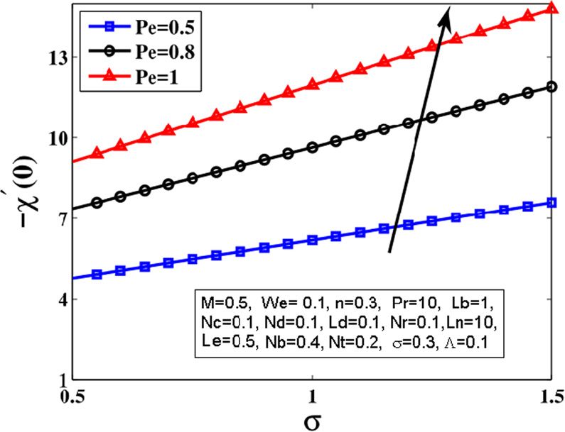
Impact of double-diffusive convection and motile gyrotactic microorganisms 75
engineering, chemistry and biology. The thermal conduc- distinct rate of diffusion. Double-diffusive convection occurs
tivity of a nanofluid is greater than that of the base fluid. in a variety of scientific disciplines such as oceanography,
The thermal conductivity of the fluid is considered to be biology, astrophysics, geology, crystal growth and chemical
enhanced by the nanoparticles present in the fluid. reactions [28]. Nield and Kuznetsov [29] scrutinized the
Buongiorno [16] established a model to examine the thermal nanofluid past a porous medium along with the double-
conductivity of nanofluids. Baby and Ramaprabhu [17] diffusive convection effect. The impact of double-diffusive
analyzed the heat transport of fluids using graphene convection on the fluid flow over a square cavity is analyzed
nanoparticles. They reported that the thermal conductivity by Mahapatra et al. [30]. Gireesha et al. [31] discussed the
of hydrogen-exfoliated graphene is enhanced with an Casson nanofluid past a stretching sheet along with the
increment in the volume fraction of the nanoparticles. MHD and double-diffusive convection. Rana and Chand [32]
Khan and Gorla [18] pondered the mass transfer of the explored the effect of double-diffusive convection on
nanofluid flow over a convective sheet using the Keller box viscoelastic fluid and deduced that a Rayleigh number
scheme and noted that the heat transfer rate is high in the increases with an improvement in the Soret parameter.
dilatant fluids compared with that in the pseudoplastic Gaikwad et al. [33] have monitored the fluid flow above a
fluids. Das [19] discussed the rotating flow of a nanofluid stretching sheet together with double-diffusive convection
with respect to the constant heat source. A boost in the and found that an augmentation in the Nusselt number
volume fraction of nanoparticles was observed to cause an takes place with an improvement in the Dufour parameter.
increment in the thermal boundary layer thickness. Gireesha Kumar et al. [34] inspected the influence of nanoparticles
et al. [20] considered the Hall impact on a dusty nanofluid and double diffusion on viscoelastic fluid and monitored
and concluded that the skin friction coefficient decreases that an increase in the velocity field occurs with an
due to an improvement in the Hall current. increment in the Dufour Lewis number.
The experimental and the theoretical scientific studies Convection is a process common to particles, gases and
of the non-Newtonian liquids together with MHD have vapours. Convection occurs when a fluid is in motion and
achieved a considerable attention of researchers because of that motion carries with it a material of interest such as the
their adequate applications in the field of aeronautics, particles or the droplets of an aerosol. There are two types of
chemical, mechanical, civil and bio-engineering. The fluid convection: free convection and forced convection. In free
becomes electrically conducting under the effect of MHD convection or natural convection, the fluid motion cannot led
like ionized gases, plasmas and liquid metals such as by external sources such as fans, pumps, and suction devices
mercury. The impact of MHD and nonlinear thermal etc. Gravity is the main driving force in the case of free
radiation on the Sisko nanofluid flow over a nonlinear convection. Free convection has various environmental and
stretching surface is premeditated by Prasannakumara industrial applications such as plate tectonics, oceanic
et al. [21]. Rashidi et al. [22] pondered the MHD viscoelastic currents, formation of microstructures during the cooling of
fluid together with the Soret and Dufour effects and molten metals, fluid flows around shrouded heat dissipation
observed that the velocity profile decreases with an fins, solar ponds and free air cooling without the aid of fans.
improvement in the magnetic parameter. Kothandapani In forced convection, the fluid motion is generated externally
and Prakash [23] studied the effect of magnetic field on with the help of pumps, fans, suction devices, etc. This
peristaltic tangent hyperbolic nanofluid past a asymmetric mechanism has enormous applications in our daily life such
channel. Gaffar et al. [24] showed the tangent hyperbolic as heat exchangers, central heating system, steam turbines
fluid flow over a cylinder together with the MHD and partial and air conditioning. Mixed convection is the situation in
slip effects. Nagendramma et al. [25] analyzed the tangent which both free convection and forced convection are of
hyperbolic fluid flow over a stretching sheet together with comparable order. Mixed convection is of great interest to
the MHD effect. Das et al. [26] investigated the impact of researchers due to its enormous applications in the industrial
magnetic field, chemical reaction and double-diffusive and engineering sectors. Ibrahim and Gamachu [35] found
convection on the Casson fluid flow past a stretching plate the numerical solution of the mixed convective Williamson
and noted that the skin friction coefficient decreases as a nanofluid past a stretching sheet by the Galerkin finite
result of an augmentation in the Grashof number. Sravanthi element method. Shateyi and Marewo [36] adopted the
and Gorla [27] examined the effect of the Maxwell nanofluid spectral quasi-linearization method to achieve the numerical
flow over an exponentially stretching sheet together with solution of the mixed convective magneto Jeffrey fluid flow
MHD, chemical reaction and heat source/sink. over an exponentially stretching sheet together with the
Double-diffusion phenomena describe a form of con- thermal radiation and observed that the fluid velocity
vection driven by two different density gradients, holding improves with an augmentation in the buoyancy parameter.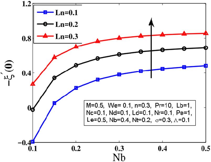
76 Tanveer Sajid et al.
Nalinakshi et al. [37] found the numerical solution of the
mixed convective fluid past a vertical stretched plate using a
nonlinear shooting method. El-Aziz and Tamer Nabil [38]
gave the numerical solution for the problem of the MHD and
Hall current effect on mixed convective fluid past a stretching
sheet using the homotopy analysis method (HAM) and noted
that a positive variation in the Hall current parameter leads to
an increase in the velocity field. Beg et al. [39] employed an
explicit finite difference scheme to yield the solution of the
magneto mixed convection nanofluid flow over a stretchable
surface under the effect of MHD and viscous dissipation. The
numerical solution of the gravity-driven Navier–Stokes
equation has been reported by Zhang et al. using a finite Figure 1: Geometry of the problem.
difference method [40]. Pal and Chatterjee [41] studied the
impact of the Soret and Dufour effects along with nonlinear nanofluid. To maintain the stability of convection, the
thermal radiation on the double-diffusive convective fluid motion of microorganisms has been taken, independent of
past a stretchable surface and achieved the numerical that of the nanoparticles. The double-diffusive fluid flow
solution for problem using the Runge–Kutta–Fehlberg over a stretching sheet embedded with gyrotactic micro-
method along with the shooting scheme. They noted that organisms has not been explored yet, and we want to
the velocity field increases with an enhancement in the rectify this problem in this study.
Grashof number. The governing equations include some important
The aim of this study was to construct a mathematical effects that have eminent involvement in the industries
model that describes a form of convection driven by two and engineering fields. The momentum equation includes
different density gradients, which have different rates of bioconvection and MHD. MHD has been used in many
diffusion (double-diffusive convection). So far, no reviews engineering processes such as nuclear reactor, MHD power
have been reported on the non-Newtonian fluid past a generation, in which heat energy is directly converted into
stretching sheet embedded with nanoparticles, double- electrical energy, Yamato-1 boat incorporating a super-
diffusive convection and motile gyrotactic microorganisms. conductor cooled by liquid helium and microfluidics. A
microorganism or microbe is an organism that is so small
that it can be seen only through a microscope (invisible to
2 Mathematical formulation the naked eye). The presence of microorganisms in the fluid
becomes the core area of the research during the past
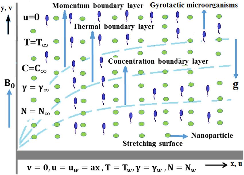
Figure 1 displays the effect of tangent hyperbolic decade. The presence of microorganisms in the base fluid
nanofluid past a stretching sheet with stretching velocity causes a “stabilization” or “destabilization” in the motion of
uw = ax along the x-axis. When the Reynolds number is nanoparticles. The microorganisms have various applica-
assumed to be small, the induced magnetic field can be tions in genetic engineering, wastewater engineering,
neglected compared with the applied magnetic field B0, agricultural engineering and chemical engineering. The
which is applied transversely to the surface. Tw, γw, Cw temperature equation and concentration equations are
and Nw denote the temperature, solute concentration, embedded with nanoparticles and double-diffusive convec-
concentration of nanoparticles and density of the motile tion. Nanoparticles are used to enhance the thermal
gyrotactic microorganisms at the wall, respectively, conductivity of the fluid and used in tissue engineering,
whereas T∞, γ∞, C∞ and N∞ denote the ambient mechanical engineering, nanomedicine, environmental en-
temperature, solute concentration, concentration of nano- gineering, etc. Double diffusion portrays the form of
particles and density of the motile gyrotactic microorgan- convection conducted by two different density gradients.
isms, respectively. The fluid has further been assumed to There are various examples in environmental engineering
contain the gyrotactic microorganisms. The microorgan- such as Arctic Ocean study and Lake Kivu, in which
isms present in the fluid move towards light. The “bottom magma, sand and materials of different densities are
heavy” mass of the microorganisms orients its body and diffused with water. The same situation is applicable in
enables them to move against the gravity g, which is called our modelled problem, in which microorganisms and
as gyrotactic phenomena. The presence of microorganisms nanoparticles of different densities are diffused together in
is considered to be beneficial for the suspension of the the fluid. The last governing equation tells us about the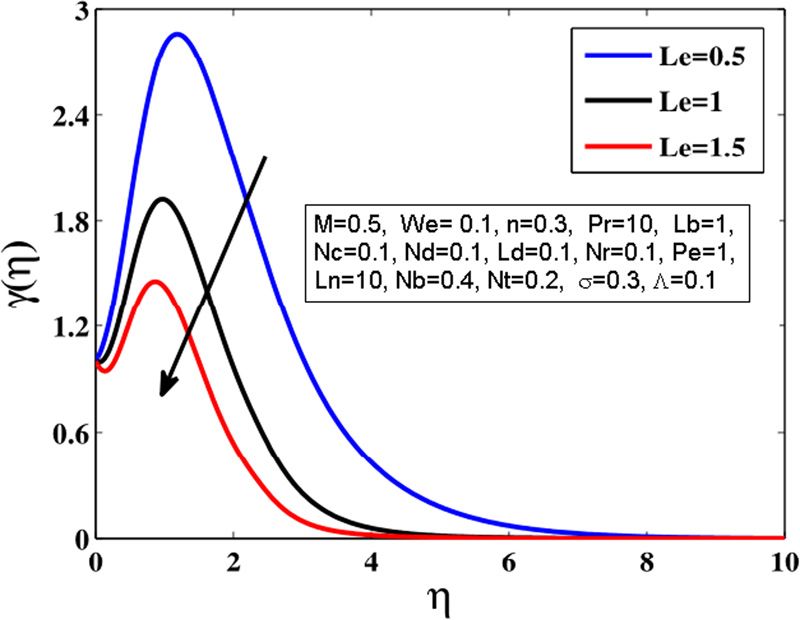
Impact of double-diffusive convection and motile gyrotactic microorganisms 77
impact of gyrotactic microorganisms present in the fluid. a
η= y, u = axf ′(η), v = − aν f (η),
Various types of microorganisms such as algae, fungi, ν
protozoa and bacteria are suspended in the fluid. These T − T∞ C − C∞
θ= , γ= , (8)
microorganisms swim in the fluid under the combination Tw − T∞ Cw − C∞
of gravitational and viscous torques (gyrotactic) in fluid ϕ − ϕ∞ N − N∞
ξ= , χ= .
flow. The gyrotactic microorganisms have enormous ϕw − ϕ∞ Nw − N∞
contribution to genetic engineering, microbial engi-
neering and soil engineering. Under the usual boundary Invoking equation (8), equation (1) is automatically
layer approximations, the equations of conservation of satisfied and equations (2)–(6) become:
mass, momentum, thermal energy, solute, concentration
of nanoparticles and gyrotactic microorganisms take the ((1 − n) + n We f ″) f ′″ − (f ′)2 + ff ″ − M2f ′
(9)
following forms [11–13,31,32,34]: + Λ (θ − Nr ξ − Nc χ ) = 0,
∂u ∂v
+ = 0, (1)
∂x ∂y θ″ + Pr (fθ′ + Nb θ′ξ ′) + Nt (θ′)2 + Nd γ″ = 0, (10)
∂u ∂u ∂ 2u ∂u ∂ 2u γ″ + Pr Le fγ′ + Ld Pr θ″ = 0, (11)
u +v = ν (1 − n) 2 + 2 Γvn
∂x ∂y ∂y ∂x ∂y 2
+ ((1 − ϕ∞) ρf gβ (T − T∞) − g (ρp − ρf )(ϕ − ϕ∞) (2)
Nt
σ ξ ″ + Pr Ln fξ ′ + θ″ = 0, (12)
− g (ρm − ρf ) γ (N − N∞)) − 1 B02 u, Nb
ρf
χ″ + Lb fχ′ − Pe (χ′ξ ′ + ξ ″(σ + χ )) = 0, (13)
∂T ∂T ∂ 2T ∂C ∂T D ∂T 2
u +v = α 2 + τ DB + T
with the following boundary conditions:
∂x ∂y ∂y ∂y ∂y T∞ ∂y (3)
∂ 2C
+ D TC 2 , f (0) = 0, f ′(0) = 1, θ (0) = 1, γ (0) = 1,
∂y
ξ (0) = 1, χ (0) = 1 at η = 0,
(14)
f ′(η) → 0, θ (η) → 0, γ (η) → 0, ξ (η) → 0,
∂ 2T χ (η) → 0 at η → ∞ .
∂C ∂C ∂ 2C
u +v = Ds 2 + DCT 2 , (4)
∂x ∂y ∂y ∂y
Distinct physical parameters arising after the con-
∂ϕ ∂ϕ ∂ 2ϕ
D
∂ 2T version of PDEs into ODEs are as follows:
u +v = DB 2 + T 2 , (5)
∂x ∂y ∂y T∞ ∂y
2a3 τDB
We = Γx , Nb = (Cw − C∞),
ν ν
∂N ∂N bWc ∂ ∂ϕ ∂ 2N D τ α
u +v + N = Dm 2 . (6) Nt = T (Tw − T∞), Le =
∂x ∂y (ϕw − ϕ∞) ∂y ∂y ∂y ,
T∞ ν Ds
α bWc α
The subjected conditions at the boundary are as follows: Ln = , Pe = , Ld = ,
DB Dm Dm
αD TC (Cw − C∞) N∞
u = uw = ax , v = 0, T = Tw, C = C w , Nd = , σ= (15)
ν (Tw − T∞) Nw − N∞
ϕ = ϕw , N = Nw at y = 0,
(7) x3 (1 − C∞) ρf gβT (Tw − T∞)
u → 0, T → T∞, C → C∞, ϕ → ϕ∞ , GT = ,
ν2
N → N∞ as y → ∞ .
ρCp (ρp − ρf )(ϕw − ϕ∞)
τ= , Nr = ,
where the symbol “ρf” depicts the fluid density and “ρp” ρCf (1 − ϕ∞) ρf β (Tw − T∞)
represents the density of nanoparticles. The similarity σB02 ν α GT
M= , Pr = , Lb = , Λ= .
transformations [38] are as follows: aρf α Dm Re2x 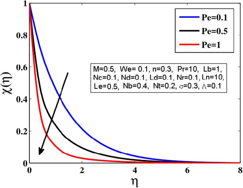
78 Tanveer Sajid et al.
The important quantities of interest like rate of shear
stress Cf and heat as well as mass transfer rates Nux and Start
Shx and Shx,n and Nnx are as follows:
Convert higher order
2τw
Cf = ,
ρu w2
xqw
Nux = ,
k (Tw − T∞)
Domain discretization
xqm
Shx = , (16)
DB (ϕw − ϕ∞)
Linearization by means of
xqmn
Shx, n = , Newton's scheme
Ds (Cw − C∞)
xqn
Nnx = , Formation of Block tri-diagonal
Dn (Nw − N∞) Aδ=R
whereas expressions regarding τw, qw, qm, qmn and qn Solution of Aδ=R by
are as follows: Block LU factorization
Updation of solution
∂u nΓ ∂u
3
τw = μ (1 − n) +μ , Stopping No
∂y y=0 2 ∂y
y=0
criteria
∂T Yes
qw = −k , Finish
∂y y=0
∂ϕ
qm = −DB , (17) Figure 2: Mechanism of the present technique.
∂y y=0
qmn = −Ds
∂C
, f ′ (η) = z1 , z ′ 1 = z2, θ′ (η) = z3, γ ′ = z4,
∂y (19)
ξ ′ = z5, χ ′ = z6
y=0
∂χ
qn = −Dn .
∂y
y=0
method (Keller box technique) [42,43] for distinguished
By substituting equation (17) into equation (16) and parameters that emerged during numerical simulation of
using the similarity transformation, the quantities defined the problem. Such type of differential equations in this
in equation (17) are nondimensionalized as follows: article can usually be solved with the help of other
numerical techniques such as shooting method, HAM and
1 1 bvp4c [27,31–34,44–49]. In this study, the standard Keller
Cf Re1 / 2 = (1 − n) f ″(0) − n We (f ″(0))3 ,
2 2 box method has been used. This numerical technique is
Nux Re−x1 / 2 = −θ′(0), quite effective and flexible to solve the parabolic-type
−1 / 2 (18) boundary value problems of any order, is unconditionally
Shx Re x = −ξ ′(0),
stable and attains remarkable accuracy. The Keller box
Shx, n Re−x1 / 2 = −γ′(0),
scheme is numerically more stable and converges using
−1 / 2
Nnx Re x = −χ′(0),
less iterations compared with other numerical techniques.
uw x
Figure 2 shows the flow chart procedure of the Keller box
where Rex = ν
. method. By adopting the new variables z1, z2, z3, z4, z5
and z6,
The dimensionless equations (9)–(13) are transformed
3 Numerical scheme
into first-order differential equations (ODEs) as follows:
The dimensionless system of equations (9)–(13) along with
the boundary condition (14) should be handled with the help ((1 − n) + n We z1) z2 − z12 + fz2 − M2z1
(20)
of the numerical scheme called the implicit finite difference + Λ (θ − Nr ξ − Nc χ ) = 0,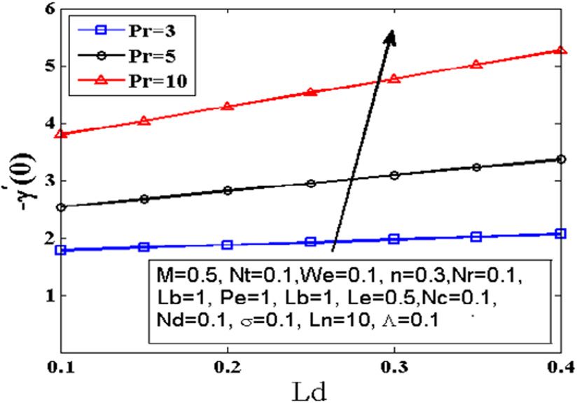
Impact of double-diffusive convection and motile gyrotactic microorganisms 79
z3′ + Pr (fz3 + Nb z3 z5) + Nt z32 + Nd z4′ = 0, (21) θj − θj − 1 (z3)j + (z3)j − 1
= , (28)
hj 2
z4′ + Pr Le fz4 + Ld Pr z3′ = 0 (22)
γj − γj − 1 (z4)j + (z4)j − 1
= , (29)
Nt hj 2
z5′ + Pr Ln z5 + z3′ = 0, (23)
Nb
ξj − ξj − 1 (z5)j + (z5)j − 1
z6′ + Lb fz6 − Pe (z6 z5 + z5′ (σ + χ )) = 0. (24) = , (30)
hj 2
The transformed boundary conditions are as follows:
χj − χj − 1 (z6)j + (z6)j − 1
f (0) = 0, z1 (0) = 1, θ (0) = 1, γ (0) = 1, = , (31)
hj 2
ξ (0) = 1, χ (0) = 1 at η = 0,
(25)
z1 (η) → 0, θ (η) → 0, γ (η) → 0, ξ (η) → 0,
χ (η) → 0 at η → ∞ .
(z2)j + (z2)j − 1
(1 − n) + n We z2
2
Figure 3 portrays the mesh structure for central 2
difference approximations. The stepping procedure for (z1)j + (z1)j − 1 (z ) + (z1)j − 1
2 1 j
− −M
the selection of the nodes in the case of domain 2 2
discretization is as follows: f j + f j − 1 (z2)j + (z2)j − 1
+ (32)
2 2
η0 = 0, ηj = ηj − 1 + ηj , j = 1, 2, 3 …, J , ηJ = ηmax .
θj + θj − 1 ξj + ξj − 1
+ Λ − Λ Nr
2 2
The derivatives of equations (20)–(24) are approximated
by employing the central difference at the midpoint ηj − 1 χj + χj − 1
− Λ Nc = 0,
2
given below: 2
fj − fj−1 (z1)j + (z1)j − 1
= , (26) (z3)j+ (z3)j − 1 (z3)j + (z3)j − 1
hj 2 + Pr
hj 2
2
fj+ fj−1 3j
(z ) + (z 3 j−1
)
(z1)j − (z1)j − 1 (z2)j + (z2)j − 1 + Nt
= , (27) 2 2 (33)
hj 2
(z3)j + (z3)j − 1 (z5)j + (z5)j − 1
+ Pr Nb
2 2
(z4)j + (z4)j − 1
+ Nd = 0,
2
(z4)j + (z4)j − 1 (z3)j + (z3)j − 1
+ Pr Ld
hj hj (34)
jf + f j−1 4 j
(z ) + (z4 j−1
)
+ Pr Le = 0,
2 2
(z5)j + (z5)j − 1 Nt (z3)j + (z3)j − 1
+
hj Nb hj (35)
f j + f j − 1 (z5)j + (z5)j − 1
+ Pr Ln = 0,
2 2
Figure 3: One-dimensional mesh for difference approximations.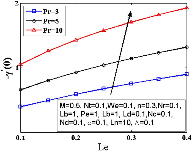
80 Tanveer Sajid et al.
(z6)j + (z6)j − 1 (z6)j + (z6)j − 1 [α1]
+ Lb [β ] [α ]
hj 2 2 2
+ fj−1 L= ⋱ ,
fj (z6)j + (z6)j − 1
− Pe
⋱ [αJ − 1]
2 2
(36) [βJ ] [αJ ]
(z5)j + (z5)j − 1 (z5)j + (z5)j − 1
− Pe
2 hj
χj + χj − 1 [I ] [ξ1]
σ + = 0,
2 [I ] [ξ2]
U= ⋱ ⋱ .
[I ] [ξJ − 1]
f jn + 1 = f jn + δf jn , (z1)nj + 1 = (z1)nj + δ (z1)nj , [I ]
(z2)nj + 1 = (z2)nj
+ δ (z2)nj , (z3)nj + 1
= +
(z3)nj δ (z3)nj ,
n+1 n n n+1 n n To solve the problem numerically, the domain of the
(z4) j = (z4) j + δ (z4) j , (z5) j = (z5) j + δ (z5) j ,
(37) problem has been considered [0,ηmax] instead of [0,∞),
(z6)nj + 1 = (z6)nj + δ (z6)nj , θjn + 1 = θjn + δθjn, where ηmax = 16 and the step size is hj = 0.01. All the
γjn + 1 = γjn + δγjn, ξ jn + 1 = ξ jn + δξ jn, numerical results achieved in this problem are subjected
χjn + 1 = χjn + δχjn . to an error tolerance of 10−5.
Table 1 displays the comparison analysis of the
given numerical scheme results with Ibrahim [40].
After linearization of the above-mentioned system of
equations, the subsequent block-tridiagonal block Table 1: Numerical comparison of the obtained results with Ibrahim
structure: [40] for various values of Pr
Pr Ibrahim [40] This study
[A1 ] [B1]
[C ] [A ] [B ] 0.00 1.0000 1.00000
2 2 2
⋱ 0.25 1.1180 1.11802
A= ⋱ , 1.00 1.4142 1.41411
⋱
[CJ − 1] [AJ − 1 ] [BJ − 1]
4 Results and discussion
[CJ ] [AJ ]
To discuss the outcomes, the behaviour of various
pertinent parameters against the Nusselt number, the
[δ1] [R1]
[δ ] [R2 ] Sherwood number, motile density profile, velocity field,
2
temperature field, mass fraction field and solute profile
⋮ ⋮
is monitored. Table 2 exhibits the behaviour of distin-
δ = ⋮ , R = ⋮
⋮ ⋮ guished parameters on heat transfer at the boundary,
mass fraction field and the motile microorganisms
[δJ − 1] [RJ − 1]
[δ ] [RJ ] density profile for thermophoresis parameter (Nt) = 0.1,
J
Prandtl number (Pr) = 6.2, Lewis number (Le) = 0.5,
Dufour Lewis number (Ld) = 0.1 and mixed convection
or
parameter Λ = 0.1. The heat transfer rate diminishes in
[A][δ] = [R], (38) the case of magnetic parameter M, Weissenberg number
(We), modified Dufour parameter (Nd), power law index
where A is the j × j tridiagonal matrix of block size 11 × n, nanofluid Lewis number (Ln) and buoyancy ratio
11, and δ and R are the column matrices of j rows. Now parameter (Nr), whereas an embellishment in the
equation (38) has been tackled using the LU factoriza- Nusselt number is seen for the Brownian motion
tion method with lower triangular matrix L and upper parameter (Nb) and the bioconvection Rayleigh number
triangular matrix U enumerated as follows: (Nc). The Nusselt number has shown no variation in the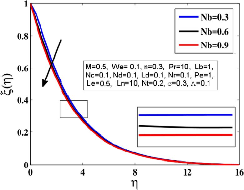
Impact of double-diffusive convection and motile gyrotactic microorganisms 81
Table 2: Variation in Nux Re−1
x
/2
, Sh ux Re−1
x
/2
and Nnx Re−1
x
/2
for different parameters when Nt = 0.1, Pr = 6.2, Le = 0.5, Ld = 0.1 and Λ = 0.1
are fixed
M Nc Nr Nb We n σ Pe Lb Nd Ln −θ′(0) −ξ′(0) −χ′(0)
0.1 0.5 0.5 0.1 0.3 0.2 0.5 1 1 0.1 2 0.93786 1.48950 1.30837
0.2 0.93815 1.50424 1.32242
0.3 0.93841 1.51812 1.33562
0.1 2.03841 2.71812 3.45016
0.3 2.03853 2.72591 2.63562
0.5 2.03865 2.73339 2.64400
0.1 2.05487 3.12893 2.93505
0.2 2.05483 3.12731 2.93360
0.3 2.05480 3.12569 2.93214
0.4 0.33911 7.72999 11.6733
0.5 0.55922 7.70119 11.6306
0.6 0.68789 7.69032 11.6146
0.1 0.82446 4.07381 6.23334
0.2 0.82438 4.06941 6.22659
0.3 0.82431 4.06476 6.21943
0.3 0.82367 4.03450 6.17277
0.4 0.82271 3.98592 6.09800
0.5 0.82134 3.90893 5.97975
0.1 0.82438 4.06941 4.69593
0.2 0.82438 4.06941 5.07859
0.3 0.82438 4.06941 5.46126
0.1 0.82438 4.06941 1.03179
0.5 0.82438 4.06941 3.31479
1 0.82438 4.06941 6.22659
0.5 0.82438 4.06941 3.31479
1 0.82438 4.06941 6.22659
1.5 0.82438 4.06941 9.18276
0.1 0.89710 2.21688 3.50681
0.2 0.81434 2.20547 3.48796
0.3 0.78569 2.18375 3.45366
1 0.89710 2.21688 3.50681
2 0.85497 3.26596 5.04071
3 0.82438 4.06941 6.22659
case of microorganism concentration difference para-
meter σ, Peclet number (Pe) and bioconvection Lewis
number (Lb). The mass fraction field depreciates in the
case of M, Nc, nanofluid Lewis number (Ln) and
buoyancy ratio parameter (Nr), but a positive variation
is observed for Nb, We, Nd and n, whereas static
behaviour is seen for σ, Pe and Lb. Furthermore, the
number of motile microorganisms has been seen to
increase in the case of positive variation in M, σ, Pe, Lb
and Ln, but the situation is opposite in the case of Nr,
Nc, n, We, Nd and Nb.
Figure 4 exhibits the effect of the magnetic para-
meter M on the velocity profile f′(η). It has been found Figure 4: Effect of parameter M on the velocity profile.
that an increase in M decreases the velocity profile.
Actually, the resistive force called the Lorentz force is of the fluid reduces. Figure 5 indicates the effect of n
generated due to the application of the magnetic field to on the velocity field f′(η). The parameter decides the
the electrically conducting fluid. As a result, the velocity viscosity of the fluid or how much viscous the fluid is.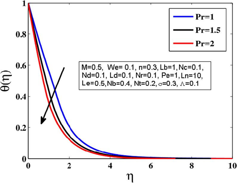
82 Tanveer Sajid et al.
Figure 5: Effect of parameter n on the velocity profile. Figure 7: Effect of parameter M on the temperature profile.
The fluid behaves like shear thinning for the case of
n < 1, shear thickening for the larger values of n > 1 and
Newtonian in the case of n = 1. The velocity of the
fluid decreases in the case of n > 1, and as a result,
the velocity field diminishes. Figure 6 depicts the effect
of f′(η) on We. The Weissenberg number is defined as the
ratio of viscous forces to the inertial forces. This
parameter is important to study the fluid flow behaviour.
The Weissenberg number actually depicts the elastic
nature of the fluid. It is noted that the higher values of
the Weissenberg number indicate the solid nature of the
fluid, while lower values of the Weissenberg number
depict the liquid nature of the fluid. It is clear that an Figure 8: Effect of parameter Pr on the temperature profile.
augmentation in the Weissenberg number leads to a
reduction in the velocity of the fluid. Figure 7 highlights
the variation in the temperature profile θ(η) against the temperature field θ(η) against Pr. The Prandtl number
various values of M and observed that an electric current is a dimensionless quantity, which is defined as the ratio
in the presence of magnetic field generates a Lorentz of momentum diffusivity to thermal diffusivity and has
force. This force resists the motion of the fluid; hence, important application in the study of boundary layer
additional heat is produced, which enhances the fluid concept. The thermal diffusivity dominates in the case of
temperature. Figure 8 highlights the behaviour of Pr ≪ 1, whereas momentum diffusivity dominates in the
case of Pr ≫ 1. It is observed that the fluids with small
Prandtl number are free flowing liquids with high
thermal conductivity and favourable choice for heat
conducting fluids. The thermal conductivity of the fluid
decreases with an augmentation in the value of Pr, and
the heat transfer decelerates, which decreases the
temperature of the flow field, and as a result, a decrease
in the temperature is observed.
Figure 9 portrays the effect of Brownian diffusion
parameter (Nb) on the temperature distribution θ(η).
Brownian motion is actually the random motion of the
particles suspended in the fluid. The temperature of the
fluid increases as a result of the random collision of
particles suspended in the liquid, which further leads to
Figure 6: Effect of parameter We on the velocity profile. an expected improvement in the temperature profile θ(η).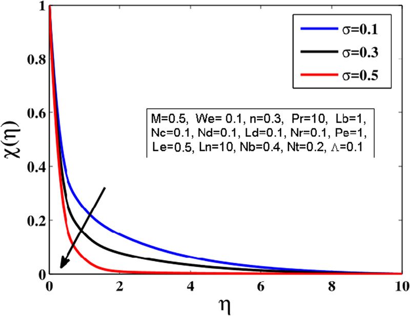
Impact of double-diffusive convection and motile gyrotactic microorganisms 83
Figure 9: Effect of parameter Nb on the temperature profile. Figure 11: Effect of parameter Nd on the temperature profile.
Figure 10: Effect of parameter Nt on the temperature profile.
Figure 12: Effect of parameter Nb on the concentration profile.
Figure 10 explores the effect of the thermophoresis
parameter (Nt) on the temperature distribution θ(η). In motion of the nanoparticles in the fluid. It is verified
the thermophoresis process, smaller particles migrate that the higher values of Nb are the root cause to boost
from the region having high temperature to the region the random motion among the nanoparticles present in
having low temperature, which ultimately causes an the fluid. This results in the decrease in the concentra-
improvement in the fluid temperature. tion of the fluid.
Figure 11 shows the behaviour of temperature profile Figure 13 describes the effect of Nt on the mass
θ(η) against the different values of Nd. The situation in fraction field. It is observed that increasing values of Nt
which heat and mass transfer happens simultaneously push nanoparticles away from the warm surface. The
in a moving fluid affecting each other causes a cross- density of the concentration boundary layer upsurges
diffusion. The mass transfer caused by temperature due to an augmentation in the value of Nt, which leads
gradient is called the Soret effect, whereas the heat to an embellishment in the mass fraction field. Figure 14
transfer caused by concentration is called the Dufour portrays the effect of the nanofluid Lewis parameter (Ln)
effect. The Dufour number implies the effect of the on the mass fraction field. The Lewis number is defined
concentration on the thermal energy flux in the flow. It as the ratio of thermal diffusivity to the mass diffusivity,
is found that a variation in the modified Dufour number and it is the prominent factor to study the heat and mass
leads to a monotonic enhancement in the temperature transfer. It is observed that the concentration profile
field θ(η). Figure 12 highlights the effect of Nb on the decreases due to the dependence of the Lewis number
mass fraction field. Brownian diffusion and thermophor- on the Brownian diffusion coefficient, which means that
esis parameters emerge as a result of an inclusion of an augmentation in the Brownian diffusion coefficient
nanoparticles into the fluid. Brownian diffusion and brings about a decrease in the concentration profile and
thermophoresis parameters help to understand the the nanofluid Lewis number.84 Tanveer Sajid et al.
Figure 13: Effect of parameter Nt on the concentration profile. Figure 16: Effect of parameter Lb on the microorganism profile.
substance moves from an area of high concentration to
an area of low concentration. It explains the movement
of the substances in the fluid. It is found that diffusivity
of microorganisms is decreased in the case of an
augmentation in Pe. As a result, the microrotation
distribution declines. Figure 16 depicts the effect of the
bioconvection Lewis number (Lb) on the microrotation
distribution. Similar to Figure 14, an augmentation in Lb
results in a decrease in the diffusivity of microorgan-
isms, which results in the reduction of the motile density
profile.
Figure 17 portrays the effect of microorganism
Figure 14: Effect of parameter Ln on the concentration profile.
concentration difference parameter σ on the motile
density profile. It is observed that by increasing the
value of σ, the concentration of microorganisms in
Figure 15 shows the effect of Peclet number (Pe) on ambient fluid is decreased. Figure 18 delineates the
the microrotation distribution χ(η). The Peclet number is effect of the regular Lewis number (Le) on the solute
the prominent factor to study the microorganisms profile γ(η). The Lewis number is defined as the ratio of
swimming in the fluid. The Peclet number is defined as thermal diffusivity to mass diffusivity. As seen in Figure 13,
the ratio of maximum cell swimming speed to diffusion the Lewis number is related to the Brownian diffusion
of microorganisms. Diffusion is the process in which a coefficient. It is observed that a positive variation in
Figure 15: Effect of parameter Pe on the microorganism profile. Figure 17: Influence of parameter σ on the microorganism profile.Impact of double-diffusive convection and motile gyrotactic microorganisms 85
concentration field. It is perceived that the concentration
gradient excites the flow with an enhancement in the
thermal energy, which results in an increase in the solute
profile. Figure 20 depicts the effect of mass fraction field on
Nb for the distinguished values of the nanofluid Lewis
number (Ln). It is also observed that due to the random
collision of molecules, the heat transfer process escalates
and nanoparticle diffusion reduces, which results in an
increment in the Sherwood number.
Figure 18: Effect of parameter Le on the solute profile.
Figure 21: Effect of parameter Nt on the Sherwood number.
Figure 21 elucidates the performance of Nt on the mass
fraction field for various values of Ln. It is found that in
the presence of the thermophoretic force, the nano-
Figure 19: Effect of parameter Ld on the solute profile. particles present close to the hot boundary have been
shifted towards the cold fluid, which decreases the
thermal boundary layer and heightens the nanofluid
Brownian diffusion leads to a decrease in the concentration Lewis number. An upsurge in Nt escalates nanofluid
of particles. Thus, a positive variation in the Lewis number Lewis number (Ln) and further leads to an augmentation
(Le) leads to a decrease in the solute profile. Figure 19 in the mass fraction field. Figure 22 presents the effect of
portrays the relationship between the Dufour Lewis number microorganism concentration difference parameter σ on
(Ld) and the solute profile γ(η). The Dufour Lewis number the density number of microrotation distribution for
depicts the influence of temperature gradient on the different values of Peclet number (Pe). A positive
Figure 20: Effect of parameter Nb on the Sherwood number. Figure 22: Effect of σ on the microorganism density profile.86 Tanveer Sajid et al.
microorganisms on the non-Newtonian fluid past a
stretching sheet. To our knowledge, no model has been
developed so far to see the impact of gyrotactic
microorganisms and double-diffusive convection simul-
taneously on the non-Newtonian hyperbolic tangent
nanofluid, and furthermore, a numerical technique
(Keller box) has been used to achieve the numerical
solution of the problem. A comparison with the previous
literature was made to check the reliability of our
proposed numerical scheme. The results are quite
promising. Some of the key findings of the present
investigation are as follows:
Figure 23: Effect of parameter Ld on the solutal Sherwood number.
• An improvement in the Weissenberg number (We)
leads to a decrease in the velocity profile.
• The mass fraction field shows an opposite behaviour
as a result of variation in the nanofluid Lewis
number (Ln).
• A positive variation in the Peclet number (Pe) leads to
a decrease in the solute profile.
• The microrotation distribution profile declines with an
improvement in the bioconvection Lewis number (Lb)
and microorganism concentration difference para-
meter σ.
• The solute profile is decreased with an enhancement
in the regular Lewis number (Le).
Figure 24: Effect of parameter Le on the solutal Sherwood number.
variation in σ lessens the thickness of the boundary
layer and leads to an increment in the concentration of Nomenclature
the motile gyrotactic microorganisms. Figure 23 eluci-
dates the conduct of the Dufour Lewis number (Ld) on a stretching rate
the solutal Sherwood number for different values of the B0 magnetic field strength
Prandtl number. The Lewis number is defined as the C∞ ambient concentration
ratio of thermal diffusivity to momentum diffusivity. It is C∞ ambient solute concentration at the wall
observed that an enhancement in Lewis number drives Cf skin friction coefficient
more heat within the fluid, which brings about an Cp specific heat
augmentation in the Prandtl number. It is noteworthy Cw solute concentration at the wall
that a positive variation in the Dufour Lewis parameter DB Brownian diffusion
leads to an augmentation in the solutal Sherwood Dm diffusivity of the microorganisms
number. Figure 24 elaborates the effect of Lewis number DT thermophoresis diffusion
(Le) on the solutal Sherwood number. It has been g gravity
observed that the solutal Sherwood number increases GT Grashof number
with an augmentation in the Lewis number. k thermal conductivity
Lb bioconvection Lewis number
Ld Dufour Lewis number
Le Lewis number
5 Concluding remarks Ln nanofluid Lewis number
M magnetic parameter
This article elaborates the effects of nanoparticles and n power law index
double-diffusive convection along with motile gyrotactic N∞ ambient density of the motile microorganismsImpact of double-diffusive convection and motile gyrotactic microorganisms 87
Nb Brownian motion inclined sheet: multiple solutions. J Taiwan Inst Chem Eng.
Nd modified Dufour parameter 2016;66:283–91.
Nt thermophoresis parameter [9] Mahdy A. Gyrotactic microorganisms mixed convection
nanofluid flow along an isothermal vertical wedge in porous
Nw density of the motile microorganisms at the wall
media. Int J Mech Aero Indus Mechatron Manuf Eng.
Pe Peclet number 2017;11(4):840–50.
Pr Prandtl number [10] Avinash K, Sandeep N, Makinde OD, Animasaun IL. Aligned
qm wall mass flux magnetic field effect on radiative bioconvection flow past a
qw wall heat flux vertical plate with thermophoresis and Brownian motion.
Defect Diffus Forum. 2017;377:127–40.
Re Reynolds number
[11] Makinde OD, Animasaun IL. Thermophoresis and Brownian
T∞ ambient temperature motion effects on MHD bioconvection of nanofluid with
Tw wall temperature nonlinear thermal radiation and quartic chemical reaction past
u,v velocity components an upper horizontal surface of a paraboloid of revolution. J Mol
Uw stretching velocity along the x-axis Liq. 2016;21:733–43.
[12] Khan WA, Makinde OD, Khan ZH. MHD boundary layer flow of
Wc cell swimming speed
a nanofluid containing gyrotactic microorganisms past a
We Weissenberg number
vertical plate with Navier slip. Int J Heat Mass Transf.
α thermal diffusivity 2014;74:285–91.
γ solute profile [13] Mutuku WN, Makinde OD. Hydromagnetic
μ dynamic viscosity bioconvection of nanofluid over a permeable vertical
ν kinematic viscosity plate due to gyrotactic microorganisms. Comput Fluids.
2014;95:88–97.
Λ mixed convection parameter
[14] Khan WA, Makinde OD. MHD nanofluid bioconvection due to
ρ density of the fluid gyrotactic microorganisms over a convectively heat stretching
ρm density of the microorganisms sheet. Int J Therm Sci. 2014;81:118–24.
ρp density of the nanoparticles [15] Makinde OD, Animasaun IL. Bioconvection in MHD nanofluid
σ microorganism concentration difference flow with nonlinear thermal radiation and quartic autocata-
σ1 electric conductivity lysis chemical reaction past an upper surface of a paraboloid
of revolution. Int J Therm Sci. 2016;109:159–71.
τw wall shear stress
[16] Buongiorno J. Convective transport in nanofluids. Int J Heat
ϕ volume fraction of the nanoparticles Trans. 2006;128(3):240–50.
[17] Baby TT, Ramaprabhu S. Enhanced convective heat transfer
using graphene dispersed nanofluids. Nanoscale Res Lett.
2011;6:289.
[18] Khan WA, Gorla RSR. Heat and mass transfer in power-law
nanofluids over a nonisothermal stretching wall with
References convective boundary condition. Int J Heat Mass Trans.
2012;134:112001.
[1] Hill NA, Pedley TJ. Bioconvection. Fluid Dyn Res. 2005;37:1. [19] Das K. Flow and heat transfer characteristics of nanofluids in a
[2] Nield DA, Kuznetsov AV. The onset of bio-thermal convection rotating frame. Alexandria Eng J. 2014;53:757–66.
in a suspension of gyrotactic microorganisms in a fluid layer: [20] Gireesha BJ, Mahanthesh B, Thammanna GT,
oscillatory convection. Int J Therm Sci. 2006;45:990–7. Sampathkumar PB. Hall effects on dusty nano fluid two-phase
[3] Alloui Z, Nguyen TH, Bilgen E. Numerical investigation of transient flow past a stretching sheet using KVL model.
thermo- bioconvection in a suspension of gravitactic micro- J Molec Liq. 2018;256:139–47.
organisms. Int J Heat Mass Transf. 2007;50:1435–41. [21] Prasannakumara BC, Gireesha BJ, Krishnamurthy MR,
[4] Sokolov A, Goldstein RE, Feldchtein FI, Aranson IS. Enhanced Ganesh KK. MHD flow and nonlinear radiative heat transfer of
mixing and spatial instability in concentrated bacterial Sisko nanofluid over a nonlinear stretching sheet. Info Med
suspensions. Phys Rev E. 2009;80(3):031903. Unlocked. 2017;99:123–32.
[5] Tsai T, Liou D, Kuo L, Chen P. Rapid mixing between ferro-nano [22] Rashidi MM, Ali M, Rostami B, Rostami P, Xie GN. Heat and
fluid and water in a semi-active Y-type micromixer. Sens mass transfer for MHD viscoelastic fluid flow over a vertical
Actuators, A. 2009;153(2):267–73. stretching sheet with considering Soret and Dufour effects.
[6] Oyelakin IS, Mondal S, Sibanda P, Sibanda D. Bioconvection Math Probl Eng. 2015;2015:1–12.
in Casson nanofluid flow with gyrotactic microorganisms and [23] Kothandapani K, Prakash J. Influence of heat source, thermal
variable surface heat flux. Int J Biomath. 2019;12:1950041. radiation, and inclined magnetic field on peristaltic flow of a
[7] Saini S, Sharma YD, Double-diffusive bioconvection in a hyperbolic tangent nanofluid in a tapered asymmetric
suspension of gyrotactic microorganisms saturated by nano- channel. IEEE Trans Nanobiosci. 2015;14:385–92.
fluid. Int J Appl Fluid Mech. 2019;12:271–80. [24] Gaffar SA, Prasad VR, Baeg OA. Computational analysis of
[8] Dhanai R, Rana P, Kumar L. Lie group analysis for biocon- magnetohydrodynamic MHD free convection flow and heat
vection MHD slip flow and heat transfer of nano fluid over an transfer of non-Newtonian tangent hyperbolic fluid from a88 Tanveer Sajid et al.
horizontal circular cylinder with partial slip. Int J Appl Comput stretching sheet in the presence of thermal radiation and
Math. 2015;1:651–75. chemical reaction. Open Phys. 2018;16:249–59.
[25] Nagendramma V, Leelarathnam A, Raju K, Shehzad A, [37] Nalinakshi N, Dinesh PA, Chandrashekar DV. Shooting
Hussain T. Doubly stratified MHD tangent hyperbolic nano- method to study mixed convection past a vertical heated plate
fluid flow due to permeable stretched cylinder. Results Phys. with variable fluid properties and internal heat generation,
2018;9:23–32. Mapana. J Sci. 2017;13:31–50.
[26] Das M, Mahanta G, Shaw S, Parida SB. Unsteady MHD [38] El-Aziz MA, Tamer Nabil T. Homotopy analysis solution of
chemically reactive double-diffusive Casson fluid past a flat hydromagnetic mixed convection flow past an exponentially
plate in porous medium with heat and mass transfer. Heat stretching sheet with Hall Current. Math Prob Engg.
transfer – Asian Res. 2019;48:1761–77. 2012;2012:26.
[27] Sravanthi CS, Gorla RSR. Effects of heat source/sink and [39] Beg OA, Khan MS, Ifsana Karim I. Explicit numerical study of
chemical reaction on MHD Maxwell nanofluid flow over a unsteady hydromagnetic mixed convective nanofluid flow
convectively heated exponentially stretching sheet using from an exponentially stretching sheet in porous media. Appl
homotopy analysis method. Int J Appl Mech Eng. Nanosci. 2014;4:943–57.
2018;23:137–59. [40] Zhang T, Salama A, Sun S, Zhong H. A compact numerical
[28] Hussain S, Mehmood K, Sagheer M, Yamin M. Numerical implementation for solving Stokes equations using matrix-
simulation of double diffusive mixed convective nanofluid vector operations. Procedia Comp Sci. 2015;51:1208–18.
flow and entropy generation in a square porous enclosure. Int [41] Pal D, Chatterjee S. Convective-radiative double-diffusion
J Heat Mass Trans. 2018;122:1283–97. heat transfer in power-law fluid due to a stretching sheet
[29] Nield DA, Kuznetsov AV. The Cheng-Minkowycz problem for embedded in non-Darcy porous media with Soret–Dufour
the double-diffusive natural convective boundary layer flow in effects. Int J Comput Methods Eng Sci Mech 2019;20:269–82.
a porous medium saturated by a nanofluid. Int J Heat Mass [42] Keller HB. Numerical methods for two-point boundary value
Trans. 2011;54:374–8. problems. New York: Dover publications; 1992.
[30] Mahapatra R, Pal D, Mondal S. Effects of buoyancy ratio on [43] Cebeci T, Bradshaw P. Physical and computational aspects of
double-diffusive natural convection in a lid-driven cavity. Int J convective heat transfer. New York: Springer Verlag; 1988.
Heat Mass Trans. 2013;57:771–85. [44] Pal D, Mondal SK. Magneto-bioconvection of Powell Eyring
[31] Gireesha BJ, Archana M, Prasannakumara BC, Gorla RSR, nanofluid over a permeable vertical stretching sheet due to
Makinde OD. MHD three dimensional double diffusive flow of gyrotactic microorganisms in the presence of nonlinear
Casson nanofluid with buoyancy forces and nonlinear thermal thermal radiation and Joule heating. Int J Ambient Energy.
radiation over a stretching surface. Int J Num Meth Heat Fluid 2019;7:3723–31.
Flow. 2018;125:290–309. [45] Khan NS. Bioconvection in second grade nanofluid flow
[32] Rana GC, Chand R. Stability analysis of double-diffusive containing nanoparticles and gyrotactic microorganisms,
convection of Rivlin-Ericksen elastico-viscous nanofluid Brazilian. J Phys. 2019;48:227–41.
saturating a porous medium: a revised model. Forsch [46] Zaman S, Gul M. Magnetohydrodynamic bioconvective flow of
Ingenieurwes. 2015;79:1–2. Williamson nanofluid containing gyrotactic microorganisms
[33] Gaikwad SN, Malashetty MS, Prasad KR. An analytical study subjected to thermal radiation and Newtonian conditions. Int
of linear and non-linear double diffusive convection with J Ambient Energy. 2019;479:22–8.
Soret and Dufour effects in couple stress fluid. Int J Non- [47] Wubshet I. MHD flow of a tangent hyperbolic fluid with
Linear Mech. 2007;42:903–13. nanoparticles past a stretching sheet with second order slip
[34] Kumar GK, Gireesha BJ, Manjunatha S, Rudraswamy NG. and convective boundary condition. Results Phys.
Effect of nonlinear thermal radiation on double-diffusive 2017;7:3723–31.
mixed convection boundary layer flow of viscoelastic nano- [48] Xua H, Pop I. Mixed convection flow of a nanofluid over a
fluid over a stretching sheet. Int J Mech Mater Eng. stretching surface with uniform free stream in the presence of
2017;12:18. both nanoparticles and gyrotactic microorganisms. Int J Heat
[35] Ibrahim W, Gamachu D. Finite element method solution of Mass Trans. 2014;75:610–63.
mixed convection flow of Williamson nanofluid past a radially [49] Reddy BSK, Krishna MV, Surya KV, Rao N, Vijaya B. HAM
stretching sheet. Heat Transfer-Asian Res. 2019;12:1–23. Solutions on MHD flow of Nano-fluid through Saturated
[36] Shateyi S, Marewo GT. Numerical solution of mixed convec- Porous medium with Hall effects. Mater Today.
tion flow of an MHD Jeffery fluid over an exponentially 2018;5:120–31.You can also read