Ships Added Mass Effect on a Flexible Mooring Dolphin in Berthing Manoeuvre

 
CONTINUE READING
Ships Added Mass Effect on a Flexible Mooring Dolphin in Berthing Manoeuvre
Journal of
               Marine Science
               and Engineering

Article
Ships Added Mass Effect on a Flexible Mooring Dolphin in
Berthing Manoeuvre
Aleksander Grm

                                           Faculty of Maritime Technology and Transport, University of Ljubljana, Pot pomorščakov 4,
                                           6320 Portorož, Slovenia; aleksander.grm@fpp.uni-lj.si; Tel.: +386-5-6767-352

                                           Abstract: This paper deals with the hydrodynamic effect of the ship on a flexible dolphin during a
                                           mooring manoeuvre. The hydrodynamic effect refers to the change in momentum of the surrounding
                                           fluid, which is defined by the concept of added mass. The main reason for the present study is to
                                           answer the question, “What is the effect of the added mass compared to the mass of the ship during
                                           the mooring procedure for a particular type of ship?” Measured angular frequencies of dolphin
                                           oscillations showed that the mathematical model can be approximated by the zero frequency limit.
                                           This simplifies the problem to some extent. The mooring is a pure rocking motion, and the 3D study
                                           is approximated by the strip theory approach. Moreover, the calculations were performed with
                                           conformal mapping using conformal Lewis mapping for the hull geometry. The fluid flow is assumed
                                           to be non-viscous, non-rotating and incompressible. The results showed that the additional mass
                                           effect must be taken into account when calculating the flexible dolphin loads.

                                           Keywords: added mass; conformal mapping; lewis mapping

                                           1. Introduction
                                       Since the beginning of naval history, ships transporting cargo or people from point
         
                                           A to point B have required facilities for safe berthing, loading, and unloading at both
Citation: Grm, A. Ships Added Mass         points A and B. Over time, ships have grown in size and specialised ships, terminals, and
Effect on a Flexible Mooring Dolphin       equipment have been built to handle specific types of cargo, such as liquid bulk, dry bulk,
in Berthing Manoeuvre. J. Mar. Sci.        and containers. For liquid bulk terminals, a jetty is the typical berthing facility. The ship is
Eng. 2021, 9, 108. https://doi.org/        usually moored at berths to dedicated breasting dolphins, which may be single-pile flexible
10.3390/jmse9020108                        dolphins or multi-pile rigid dolphins with fenders.
                                                 The primary objective of this work is to estimate the ship added mass. A typical
Received: 22 December 2020
                                           situation of this research geometry and motion is shown in Figures 1 and 2. A ship is
Accepted: 18 January 2021
                                           moving in a pure sway direction with a constant speed towards the pier. To avoid direct
Published: 21 January 2021
                                           contact with the infrastructure of the liquid cargo terminal, two flexible dolphins reduce
                                           the speed of the ship and act as two huge shock absorbers. The current cargo terminal was
Publisher’s Note: MDPI stays neu-
                                           designed for smaller types of ships, but now larger ships also call at the Port of Koper. As
tral with regard to jurisdictional clai-
                                           far as safety is concerned, it is also about the safety of the docking process. In the safety
ms in published maps and institutio-
nal affiliations.
                                           analysis of the docking manoeuvre, many different factors need to be analysed in order to
                                           get a complete picture of the ship dynamics and the response of the port infrastructure. In
                                           this article, we focus exclusively on the estimation of the added mass for such an operation.
                                                 Hydrodynamic modelling of added mass phenomena goes way back to names such
Copyright: © 2021 by the author. Li-       as Green, Stokes, etc. The influence of added mass has been expressed mathematically and
censee MDPI, Basel, Switzerland.           accurately by the expression of the added mass of a sphere. The influence of a free surface
This article is an open access article     on the added mass for surface piercing bodies began many years later. For a given ship,
distributed under the terms and con-       it can be determined by an experimental method. However, the experimental method is
ditions of the Creative Commons At-        limited to a certain condition. To simulate the ship motion, especially in the initial stage of
tribution (CC BY) license (https://
                                           design, the added mass must be calculated by a theoretical method.
creativecommons.org/licenses/by/
4.0/).

J. Mar. Sci. Eng. 2021, 9, 108. https://doi.org/10.3390/jmse9020108                                              https://www.mdpi.com/journal/jmse
J. Mar. Sci. Eng. 2021, 9, 108                                                                                                     2 of 21

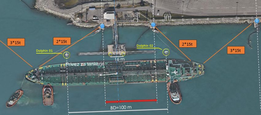
                                 Figure 1. View of the berth in Port of Koper. The dolphins are to the right and the left from the central
                                 pier-yellow circles on the sea (photo M.Perkovic).

                                                     V                       c
                                                                         F
                                                  M+m22

                                                                                         b

                                                                                 er
                                                                           ay
                                                                         eL
                                                                      on
                                                                    St

                                                                                         a
                                                         Mud Region

                                                      Stone Layer

                                 Figure 2. Flexible dolphin mooring with all dimensions. The bottom structure consists of different
                                 layers of material: Stones and mud. A ship with mass M + m22 and velocity V approaches the
                                 mooring. The dolphin is curved by c and the force acting at this moment is F.

                                      The principal for calculating the added mass for surface piercing bodies began with
                                 the work of Ursell [1,2] for a cylindrical cross-section. The mathematical model is based on
                                 the multipole expansion approach and is in some sense restricted to simple cross-sectional
                                 geometries and infinite water depth. The extension of the model to shallow water goes
                                 back to Thorne [3]. An important work by Ursell and co-authors can be found in [4].
                                 The multipole expansion method was later used by many researchers, in particular it is
                                 very attractive for those working in theoretical hydrodynamics. The completely different
                                 approach began with Frank [5], who developed a method for arbitrary cross-sections based
                                 on the integral equation approach. The problem can be solved in the frequency domain,
                                 introducing a linear consideration of all quantities involved. However, the mean drift
                                 forces of order 2nd can only be obtained with the linear solution, e.g., [6]. In addition, Inglis
                                 and Price [7], Newman and Sclavounos [8], and Nakos and Sclavounos [9] are among the
                                 most important studies of this type.
                                      All of the above methods implement the potential flow assumption and completely
                                 neglect viscous effects. The added mass can typically be approximated as not depending
J. Mar. Sci. Eng. 2021, 9, 108                                                                                            3 of 21

                                 on viscosity for the particular case of sinusoidal relative motion between the flow and
                                 the object [10]. Similarly, viscous effects are negligible for radiated gravity waves due
                                 to body motion, but the same is not always true for damping. It is known that viscous
                                 damping during roll is typically the most significant viscous effect on the motion of a ship.
                                 Lavrov et al. [11] performed CFD calculations using the Navier-Stokes equations with the
                                 k − ω turbulence model to study the flow in the vicinity of 2D ship sections subjected to
                                 forced rolling motions. They concluded that for the same shapes, a 10–20% difference in
                                 added mass was observed over the entire frequency range compared to results from using
                                 a linear frequency domain potential flow code.
                                      The approach taken in the present study is more in line with the Ursell method,
                                 combined with the Conformal Mapping approach. Lewis [12] proposed the classical
                                 extended Joukowski transformation method, creating the two-parameter Lewis family
                                 of ship-like sections. The family was extended by Landweber and Macagno [13,14] to
                                 include an additional parameter, the second moment of the cross-sectional area about
                                 the horizontal x-axis. Ursell’s approach was used extensively in ship hydrodynamics
                                 by Grim [15], Tasai [16], Porter [17], De Jong [18] and others. Later, Athanassoulis and
                                 co-authors [19–21] extended this approach to unsymmetric sections as well. It should be
                                 noted that the use of only three parameters leads to a quite satisfactory description of ship
                                 sections of conventional hull shapes, as is the case here. This property was exploited, for
                                 example, by Grigoropoulos and Loukakis [22,23] to optimize the hull shape in terms of
                                 the seakeeping.
                                      The problem of determining added mass traditionally falls within the scope of ship
                                 manoeuvrability analysis [24–26]. The manoeuvrability of a ship under various conditions
                                 has been studied by several authors [27–31] and many others. The most complex theories of
                                 manoeuvring and seakeeping involve nonlinear wave loads with higher-order effects [25].
                                 In our case, it is possible to simplify most of the complex theory. Incoming waves are
                                 neglected since the ships sail in mostly closed waters. The measured periods of ship motion
                                 are very small [32], so a common approach is to further simplify the motion at a zero
                                 frequency limit. In this case, only radiated terms are relevant. A similar approach with
                                 experimental setup was also studied in [33,34].
                                      The underlying fluid model is nonviscous, nonrotating, and incompressible to simulate
                                 flow around the hull. The ideal flow is represented by a complex velocity potential for the
                                 channel geometry (the bottom boundary is included in the geometry—Figure 3). Using
                                 the theory of complex functions with conformal mapping, it is possible to solve the flow
                                 problem of a complex geometry in a simplified geometry [35–37]. In this study, a cylindrical
                                 geometry is mapped to a hull geometry using Lewis mapping [12]. The complex velocity
                                 potential is integrated over the simplified geometry to obtain the added mass coefficient.
                                 The strip theory approach [38] simplifies the 3D problem to a set of 2D problems. The
                                 added mass is calculated for three representative ships: Middle Range oil tanker (MR) with
                                 range 25,000 t–55,000 t, Long Range type one oil tanker (LR1) with range 55,000 t–80,000 t
                                 and Long Range type 2 oil tanker (LR2) with range 80,000 t–160,000 t. The analysis of the
                                 under kill clearance (UKC) effect is also studied. For each type of ship, the velocity field is
                                 calculated for 20 different drafts from the summer waterline at the intervals of 0.1 m.
J. Mar. Sci. Eng. 2021, 9, 108                                                                                            4 of 21

                                                                B

                                                              V = ẋ
                                                                             x   Γw
                                  ∞                                                                 ∞
                                                                 θ                    x = ρ sin θ
                                                                             ρ        y = ρ cos θ

                                             T                      y            Γs
                                        Hw                                            z = x + iy
                                                        Fhy = (M + m22 )V̇            z = iρ exp(−iθ)

                                                                                        Ω

                                             Hb - UKC
                                  ∞                                              Γb                 ∞

                                 Figure 3. Description of the computational domain.

                                 2. Formulation of the Problem
                                       The added mass is associated with the change in momentum of the surrounding fluid
                                 over time [24]. If the fluid is ideal (non-viscous and irrotational) and incompressible, then
                                 the fluid is completely described by the complex velocity potential Φ in 2D [39]. Consider
                                 a two-dimensional ideal and incompressible fluid in a bounded geometry Ω bounded
                                 by the water surface (Γw ), the bottom (Γb ) and the hull (Γs ), as shown in Figure 3. In
                                 the ( x, y) coordinate system (Figure 3), the velocity potential Φ(x , t), where x = ( x, y) is
                                 a point in domain Ω, for a moving body in an otherwise still fluid can be given by the
                                 differential equation

                                                                             ∂2 Φ ∂2 Φ
                                                                                 + 2 = 0, x ∈ Ω                              (1)
                                                                             ∂x2  ∂y
                                 and the boundary conditions

                                                                          ∂Φ
                                                                             + k Φ = 0,              x ∈ Γw                (2a)
                                                                          ∂y
                                                                            n · ∇Φ = 0,              x ∈ Γb                (2b)
                                                                         n · ∇Φ = n · V ,            x ∈ Γs                 (2c)

                                 where n is the normal unit vector always pointing out of domain Ω and k is a wavenumber
                                 defined by the relation k = ω 2 /g (infinite depth [26]), where ω is the frequency of the
                                 oscillating body, g is the acceleration due to gravity, and V is the velocity of the body.
                                 Furthermore, the velocity potential for the oscillatory phenomena can be written in the form
                                                                                          
                                                                  Φ(x , t) = < φ(x )e−iωt ,                                (3)

                                 where the potential Φ is split into the temporal (e−iωt ) and spatial components (φ(x )). It
                                 can be shown that the system (1)–(2) is also valid for φ [26].
                                      In the case we study, the oscillations are very slow (ω  1), so the boundary
                                 condition (2a) can be simplified to

                                                               ∂Φ
                                                                  = n · ∇Φ = 0, x ∈ Γw (for k → 0).                          (4)
                                                               ∂y

                                 Now, the solution φ must satisfy the following system

                                                                        ∂2 φ ∂2 φ
                                                                            + 2 = 0,                  x∈Ω                  (5a)
                                                                        ∂x2    ∂y
                                                                            n · ∇φ = 0,             x ∈ Γw , Γb            (5b)
                                                                        n · ∇φ = n · V ,              x ∈ Γs                (5c)
J. Mar. Sci. Eng. 2021, 9, 108                                                                                                 5 of 21

                                  where the boundary notations are shown in Figure 3. The ship moves with velocity V in x
                                 (sway) direction according to the orientation of the coordinate system shown in Figure 3.
                                 The fluid flow can be represented by the potential φ as a moving dipole potential for a
                                 body described by a cylindrical shape [24].
                                      Let us convert the ( x, y) coordinate system into the complex notation

                                                                   z = x + iy, x, y ∈ R, z ∈ C.                                   (6)

                                 Such a representation simplifies the solution procedure. It is always possible to write the
                                 complex velocity potential as the sum of two real-valued functions

                                                                    Φ(z) = φ( x, y) + iψ( x, y),                                  (7)

                                 where we have the fluid velocity defined as the gradient of the real part of the complex
                                 potential [26]
                                                              v := ∇
J. Mar. Sci. Eng. 2021, 9, 108                                                                                                                6 of 21

                                 where discussed parameters are shown in Figure 3. Velocity is a time-dependent quantity
                                 and the potential can be decomposed as

                                                                                                                                dφ
                                                                                              φ = V φ̃               →             = V̇ φ̃,    (13)
                                                                                                                                dt
                                 assuming that the velocity V and potential φ̃ are related to the velocity and potential in the
                                 sway direction [26].

                                      Typical solutions of Equation (10) for variables φ and ψ can be seen in Figures 4–9,
                                 for V = 1 and various h in the case of a cylindrical body geometry. Let us further rewrite
                                 the coordinate system into a more natural one for cylindrical geometry. The transforma-
                                 tion from Cartesian coordinates ( x, y) to polar coordinates (ρ, θ ) with the notation of the
                                 complex plane is

                                                                                   x =ρ sin θ, y = ρ cos θ, x, y, ρ, θ ∈ R                    (14a)
                                                                                   z = x + iy = iρ exp(−iθ ), z ∈ C                           (14b)

                                 as can be seen in Figure 3. The geometry of the cylindrical body can be transformed into a
                                 shape similar to the ship-like shape using the conformal mapping w = f (z), preserving
                                 the shape of the complex velocity potential Φ(z) [35]. This fact is used to compute the
                                 hydrodynamic force in the cylindrical geometry Ωc of the flow generated by the ship
                                 geometry Ωs Figure 10.

                                     0
                                  -0.2
                                  -0.4
                                  -0.6
                                  -0.8
                                    -1
                                  -1.2
                                         -3             -2           -1             0              1                 2              3

                                                −2.16    −1.62   −1.08    −0.54    0.00     0.54       1.08   1.62       2.16

                                     0
                                  -0.2
                                  -0.4
                                  -0.6
                                  -0.8
                                    -1
                                  -1.2
                                         -3             -2           -1             0              1                 2              3

                                              −0.615    −0.540   −0.465   −0.390   −0.315    −0.240      −0.165   −0.090        −0.015

                                 Figure 4. Plot of Equation (10) in the form (7). The top plot shows the real part of the complex
                                 potential φ( x, y), the bottom plot shows the imaginary part of the complex potential ψ( x, y) for
                                 velocity V = 1 and channel gap width h = 1.2 for cylindrical geometry Γs with ρ = 1.
J. Mar. Sci. Eng. 2021, 9, 108                                                                                                                                                    7 of 21

                                     0
                                  -0.2
                                  -0.4
                                  -0.6
                                  -0.8
                                    -1
                                  -1.2
                                          -3                     -2                 -1                   0                      1                          2                  3

                                              0.08      0.40           0.72        1.04      1.36            1.68        2.00             2.32         2.64        2.96
                                  0.0

                                 −0.5

                                 −1.0

                                               −3                 −2                  −1                     0                  1                       2                 3

                                 Figure 5. Plot of the Equation (8). The top plot shows the velocity amplitude kv k, the bottom plot
                                 shows the velocity vector field for velocity V = 1 and the channel gap of width h = 1.2 for cylindrical
                                 geometry Γs with ρ = 1.
                                    0

                                  -0.5

                                   -1

                                  -1.5

                                   -2
                                         -3                 -2                -1                  0                 1                     2                    3

                                                     −1.2    −0.9         −0.6      −0.3      0.0        0.3            0.6         0.9          1.2

                                    0

                                  -0.5

                                   -1

                                  -1.5

                                   -2
                                         -3                 -2                -1                  0                 1                     2                    3

                                              −0.92    −0.82          −0.72   −0.62       −0.52       −0.42      −0.32        −0.22        −0.12       −0.02

                                 Figure 6. Plot of the Equation (10) in the form (7). The top plot shows the real part of the complex
                                 potential φ( x, y), the bottom plot shows the imaginary part of the complex potential ψ( x, y) for
                                 velocity V = 1 and channel gap width h = 2.0 for cylindrical geometry Γs with ρ = 1.

                                     0

                                  -0.5

                                    -1

                                  -1.5

                                    -2
                                          -3                     -2                 -1                   0                      1                       2                 3

                                              0.03      0.18           0.33      0.48       0.63        0.78        0.93            1.08         1.23          1.38

                                  0.0

                                 −0.5

                                 −1.0

                                 −1.5

                                 −2.0
                                               −3                 −2                −1                   0                      1                      2                  3

                                 Figure 7. Plot of the Equation (8). The top plot shows the velocity amplitude kv k, the bottom plot
                                 shows the velocity vector field for velocity V = 1 and the channel gap of width h = 2.0 for cylindrical
                                 geometry Γs with ρ = 1.
J. Mar. Sci. Eng. 2021, 9, 108                                                                                                               8 of 21

                                  0
                                  -1
                                  -2
                                  -3
                                  -4
                                  -5
                                       -10                      -5                    0                         5                       10

                                             −0.900    −0.675    −0.450   −0.225    0.000     0.225     0.450       0.675     0.900

                                  0
                                  -1
                                  -2
                                  -3
                                  -4
                                  -5
                                       -10                      -5                    0                         5                       10

                                              −0.92     −0.82    −0.72    −0.62    −0.52    −0.42     −0.32    −0.22    −0.12    −0.02

                                 Figure 8. Plot of the Equation (10) in the form (7). The top plot shows the real part of the complex
                                 potential φ( x, y), the bottom plot shows the imaginary part of the complex potential ψ( x, y) for
                                 velocity V = 1 and channel gap width h = 5.0 for cylindrical geometry Γs with ρ = 1.

                                  0
                                  -1
                                  -2
                                  -3
                                  -4
                                  -5
                                       -10                      -5                    0                         5                       10

                                        0.025     0.150         0.275     0.400    0.525      0.650      0.775       0.900      1.025

                                  0

                                 −2

                                 −4

                                       −10.0          −7.5      −5.0       −2.5       0.0       2.5           5.0       7.5           10.0
                                 Figure 9. Plot of the Equation (8). The top plot shows the velocity amplitude kv k, the bottom plot
                                 shows the velocity vector field for velocity V = 1 and the channel gap of width h = 5.0 for cylindrical
                                 geometry Γs with ρ = 1.
J. Mar. Sci. Eng. 2021, 9, 108                                                                                                  9 of 21

                                                         w = f (z)

                                          Ωc                                 Ωs

                                      z = x + iy                        w = u + iv
                                        Φ(z)                          Φ̃(w) = Φ(f (z))

                                 Figure 10. Conformal mapping w = f (z) of a circular domain Ωc onto a ship-like domain Ωs with
                                 coordinates and velocity complex potentials preserved by the mapping.

                                      One of the most commonly used conformal mappings for ship-like forms is the Lewis
                                 transformation [12], which uses only 3 free parameters a, a1 and a3
                                                                   a     a3 
                                                        w = a z + 1 + 3 , z ∈ C, a, a1 , a3 ∈ R,                    (15)
                                                                    z     z
                                 where a only causes the shape to expand/compress, but does not affect the appearance of
                                 the shape. The free parameters are determined with the basic parameters of the specific
                                 ship cross-section: B—maximal breadth, T—draft and S—area

                                                                S
                                                            σs =  ,                                                             (16a)
                                                               BT
                                                                B
                                                           H= ,                                                                 (16b)
                                                               2T
                                                                                     H−1 2
                                                                                    
                                                                    4σs       4σs
                                                           C1 = 3 +      + 1−              ,                                    (16c)
                                                                     π         π     H+1

                                                                 B
                                                             a = (1 + a1 + a3 ),                                                (16d)
                                                                 2
                                                                          H−1
                                                            a1 =(1 + a3 )      ,                                                (16e)
                                                                          H+1
                                                                            √
                                                                 −C1 + 3 + 9 − 2C1
                                                            a3 =                   .                                            (16f)
                                                                          C1

                                      Figure 11 and Table 1 show the data used in the present calculations. The ship
                                 constructed from these cross-sections is referred to as the Lewis ship. The hydrodynamic
                                 properties of sway motion for the Lewis ship are shown in Figure 12 for infinite depth and
                                 in Figure 13 for finite depth.

                                 Table 1. Lewis mapping coefficients for MR, LR1 and LR2 oil tanker type with Cb = 0.78 producing
                                 shapes in Figure 11. Only Bk needs to be scaled with β = B/T ratio for different draft calculations.

                                     Section (k)             Bk                   Tk                 σk                  L̃k
                                          0                  0.8                  0.2                0.60                0.05
                                          1                  1.2                  0.9                0.50                0.05
                                          2                  1.6                  1.0                0.68                0.05
                                          3                  2.0                  1.0                0.93                0.05
                                          4                  2.0                  1.0                0.99                0.60
                                          5                  2.0                  1.0                0.93                0.05
                                          6                  1.8                  1.0                0.68                0.05
                                          7                  1.2                  1.0                0.56                0.05
                                          8                  0.3                  0.7                0.56                0.05
J. Mar. Sci. Eng. 2021, 9, 108                                                                                                                   10 of 21

                                                              Aft sections                                              Forward sections
                                 0.0                                                                  0.0

                                 0.2                                                                  0.2

                                                                                            0                                     4
                                 0.4                                                                  0.4
                                                                                            1                                     5
                                                                                            2                                     6
                                 0.6                                                        3         0.6                         7
                                                                                            4                                     8

                                 0.8                                                                  0.8

                                 1.0                                                                  1.0

                                         1.0       0.8        0.6       0.4        0.2     0.0              0.0   0.2     0.4     0.6      0.8   1.0

                                 Figure 11. Ship cross-sections used in the calculation. The parameters of the cross-section are shown
                                 in Table 1.

                                                         Cross section parameters - infinite depth (h = ∞)

                                       101

                                       100

                                                                                           (k)
                                                                                          c22
                                   10−1                                                   Sk
                                                                                          B/T

                                               0          1         2         3          4        5   6       7     8
                                                                                  Cross section k

                                                                                                                                                       (k)
                                 Figure 12. Results for Lewis cross-sections k from Table 1 (Figure 11) for infinite water depth. c22 is
                                 the added mass coefficient, B/T is the ratio of beam/draft cross-section, and Sk is the cross-section
                                 area. The scales on the ordinate are logarithmic for better result representation.
J. Mar. Sci. Eng. 2021, 9, 108                                                                                                   11 of 21

                                                 Lewis ship added mass coefficient - infinite depth (h = ∞)

                                       1.0

                                       0.9

                                       0.8

                                       0.7
                                 c22

                                       0.6

                                       0.5

                                       0.4

                                       0.3

                                             2           3         4          5                  6               7       8
                                                                             B/T

                                 Figure 13. Results for Lewis ship defined in Table 1 (Figure 11) for infinite water depth. c22 is the
                                 added mass coefficient for the Lewis ship, and B/T is the ratio between beam and draft.

                                      The hydrodynamic force resulting from the time variation of the surrounding fluid is
                                 defined in [24] and is equal to

                                                                                      d
                                                                                           Z
                                                                        F =−ρ                        φ n dS
                                                                                      dt       Γs
                                                                                      Z
                                                                                 −ρ                  (n · ∇φ) ∇φ dS                (17)
                                                                                          Γw ∪Γb
                                                                                      1
                                                                                           Z
                                                                                 +ρ                     (∇φ · ∇φ) n
                                                                                      2        Γw ∪Γb

                                 In the present study, the integrals over the boundary Γw ∪ Γb are zero, since we are only
                                 interested in the sway component of the motion. Splitting the potential φ into a velocity
                                 part and a space part (13) gives the final form of the hydrodynamic force
                                                                                                      Z
                                                                             F = −ρ V̇ V                       φ̃ n dS
                                                                                                          Γs
                                                                                                                                   (18)
                                                                                 = −V̇ ρ V c22
                                                                                 = −V̇ m22 ,

                                 where V is the displacement of the body, ρ is the fluid density, V̇ is the acceleration of
                                 the body, c22 is added mass coefficient in sway mode, and m22 is the added mass in sway
                                 mode. To calculate the integral over the body surface Γs , we perform the integration for
                                 each cross-section k according to Table 1 and add their contribution to the total added
                                 mass. The coefficient of the added mass for each cross-section k is calculated in the circular
                                 cross-section in space Ωc and transferred to the ship cross-section in space Ωs using the
                                 conformal mapping (15). The integral in (18) is transformed from Ωc to Ωs

                                                                        2                                            dw dz
                                                                            Z π/2
                                                                 (k)
                                                                c22 =               φ̃(w) (n (w) · e x )                   dθ,     (19)
                                                                        S    0                                       dz dθ
                                 where w = f (z) is a conformal mapping (15), z = z(ρ, θ ) is defined in (14b), e x is a unit
                                 vector in x (sway) direction in Ωs (Figure 3), and S is the area of the cross-section k. The
                                 integral (19) is computed as a contour integral over the cylinder in the polar coordinates
                                 with radius ρ = 1 and θ ∈ [0, π/2]. The term dw/dz is the Jacobian of the conformal
                                 mapping and dz/dθ follows from the chain rule in the derivative of conformal mapping.
J. Mar. Sci. Eng. 2021, 9, 108                                                                                                    12 of 21

                                 The potential in (19) is written in dimensionless form. The length scale is scaled by Ti
                                 (specific draft configuration) and the velocity by the ship velocity V according to the
                                 following scheme

                                                   x = x̃Ti ,                               y =ỹTi ,                              (20a)
                                                   ẋ =ṽ x V,                              ẏ =ṽy V,                             (20b)
                                                                2                                        2
                                                   ẍ = ã x V /Ti ,                        ÿ = ãy V /Ti .                       (20c)

                                      The added mass of a cross-section k is given by the cross-section k added mass
                                 coefficient (19) multiplied by the respective water density ρ and volume Vk

                                                                      (k)    (k)            (k)
                                                                    m22 = c22 ρ Vk = c22 ρ (S̃k BTi ) ( L̃k L),                     (21)

                                 where S̃k is the dimensionless cross-sectional area and L̃k is the dimensionless cross-
                                 sectional length. For each cross-section k the values for S̃k and L̃k are taken from Table 1,
                                 and for each ship type, the constants B, Ti and L are taken from Table 2. The final added
                                 mass of the ship for the slow sway motion is the sum of all added mass contributions of
                                 the cross-sections k
                                                                                            8
                                                                                                   (k)
                                                                                   m22 =   ∑ m22 .                                  (22)
                                                                                           k =0

                                 Detailed description of added mass calculation procedure is described in next section.

                                 Table 2. Oil tanker types used in simulation: L = Lbp —length between perpendiculars, B—maximal
                                 breadth, Tmax —draft at summer line, Tmin —minimal draft in simulation, Cb block coefficient. Specific
                                 draft Ti is in the interval [Tmin ,Tmax ].

                                      Type              L [m]                 B [m]               Tmin [m]     Tmax [m]      Cb
                                       MR               185.0                  29.1                 8.50          10.50     0.78
                                       LR1              220.0                  36.3                10.50          12.50     0.78
                                       LR2              238.0                  41.3                12.20          14.20     0.78

                                 3. Results
                                      The ship moves at a relatively slow speed when docked. In this study, the problem’s
                                 formulation contains many reasonable simplifications to obtain results based only on
                                 symbolic derivations. The further simplification of the full 3D problem is based on the
                                 strip theory approach. The first step was to decompose the representative geometry of
                                 the oil tanker into some cross-sections to obtain relevant shape differences. The Levis
                                 map (15) is used to describe different cross-sections. The generated data for each cross-
                                 section describing the shape of the oil tanker are shown in Table 1. The results can be seen
                                 in Figure 11.
                                      In Figures 4–9 are plots of the complex dipole potential (10) for different values of
                                 the water height h, where ρ = 1 and V = 1. The sequence of images for different h shows
                                 the difference between the deep water solution (h >> 1) and the shallow water solution
                                 ((h − 1) < 1. The gap effect can be well observed from the intensity of the velocity potential
                                 φ. The maximum value is in the range from 2.5 to 1.2, for water heights from h = 1.2 to
                                 h = 5.0. The magnitude of the velocity in the gap increases with smaller h. The higher
                                 values of φ at the cylinder boudary result in a larger additional mass. The magnitude of
                                 the velocity in the gap is related to the viscous damping. The larger the magnitude of the
                                 velocity in the gap, the smaller the gap width and the stronger the viscous forces act.
                                      Three different representative oil tanker types are studied for the selection of ship
                                 types. The different types show the difference in the added mass in terms of ship size, their
                                 particulars, and UKC distance. The influence of UKC on the added mass was determined
                                 with 20 different ship drafts Ti . In this case, the number of draft subdivisions is not a
J. Mar. Sci. Eng. 2021, 9, 108                                                                                                   13 of 21

                                 limit, since the calculations for a single geometry are very fast (order of magnitude of
                                 a few seconds). Table 2 gives the main specifications for the different oil tanker types
                                 used in the simulation. All three types have the same block coefficient Cb = 0.78 with the
                                 cross-sectional shapes defined in Table 1 and their particulars defined in Table 2.
                                      To obtain the Lewis cross-sectional forms for various drafts Ti , we only need to
                                 multiply the coefficient Bk in Table 1 by the constant β i

                                                                                                      B/Ti
                                                                         Bk → β i Bk , β i =               .                        (23)
                                                                                                       2
                                      The ratio β i is defined as the ratio between the ship’s beam B and the current ship’s
                                 draft Ti and the constant ratio B/T = 2 for the Lewis ship ( Table 1). The values of a given
                                 ship configuration “i” (B/Ti ) are calculated from Table 2. The cross-sectional area Sk for a
                                 given configuration i is determined as

                                                                              Sk = σk β i Bk Tk ,

                                 where k = {0, 1, . . . , 8} is the cross-section number and i = {1, 2, 3, 4, . . . , N } is the specific
                                 draft configuration, where N is the number of different draft scenarios for a given tanker
                                 type. In the present case, N was set to 20 to get nice continuous plots. The calculations are
                                 very fast, and it takes about SI 1s to calculate a single draft configuration. One of the main
                                 considerations in the present work was also the speed of the computation, and it could
                                 only be achieved with a semi-analytical approach.
                                      In the previous section, a complete model for calculating the added mass in slow
                                 sway motion was formulated. The model is based on a potential flow theory with linear
                                 boundary conditions (5). For simple geometries, such as the circular one, the solution φ
                                 of (5) is a pulsating dipole with origin at the free surface (10) with constant A defined
                                 in Equation (11). The solution (10) satisfies the PDE system (5) only for a circular body
                                 geometry. The added mass coefficient c22 of a circular geometry can be easily obtained
                                 using the integral (18) for different water heights h. Figure 14 shows the solution for the
                                 added mass coefficient as a function of different dimensionless gap widths (UKC/R). For
                                 this particular case, one obtains the explicit expression for the added mass coefficient

                                                              2 π/2
                                                                  Z
                                                    c22 (h) =       φ̃ sin θ dθ
                                                              S 0
                                                                                          π 
                                                              4 π/2      2h
                                                               Z
                                                                                2 π
                                                                                  
                                                            =       <       sinh     coth     z sin θ dθ,                           (24)
                                                              π 0        π        2h       2h

                                                                z → i exp(−iθ )
                                                                         "                 2 #
                                                                             1         2h                  π
                                                             c22 (h) ≈         +                   sinh2      , h > 1,
                                                                             3         π                   2h                       (25)
                                                                  h = 1 + UKC/R,
                                 where the term coth( x ) in the integral function (24) has been expanded into Taylor series
                                 (see [40]). For |z| = 1 the series converges very quickly. Already the first three terms
                                 yield the solution error below 10−3 . To obtain the added mass coefficient, the value of
                                 the integral must be divided by the area of the cross-section. In this particular case for a
                                 circular cross-section with unit radius, the value of the area is S = (πR2 )/2 = π/2. The
                                 result shown in Figure 14 will be used later when verifying the results of the proposed
                                 method for calculating the added mass of a tanker-type ship.
                                      The average water depth at the liquid terminal in the Port of Koper is approximately
                                 Hw = 14.5 m. The variable h is calculated using Equation (12) for different Lewis shapes
                                 (Table 1) and ship particulars (Table 2) for each draft configuration Ti . If h is known, the
J. Mar. Sci. Eng. 2021, 9, 108                                                                                                          14 of 21

                                 coefficient of added mass coefficient c22 , as defined in Equation (19), can be calculated for
                                 each cross-section k

                                                                               2                                    dw dz
                                                                                    Z π/2
                                                                       (k)
                                                                      c22 =                  φ̃(w) (n (w) · e x )         dθ.
                                                                               S      0                             dz dθ
                                 Now each term of the integral is explained in detail. Let us begin with the velocity potential
                                                                          π 
                                                      2h         π
                                         φ̃(w) = <        sinh2      coth     w
                                                      π         2h         2h
                                                                                                 
                                                      2h         π        π       a      a3 
                                               =<         sinh2      coth     a z+ 1 + 3            , z → i exp(−iθ ),
                                                      π         2h         2h        z     z
                                                           2 π         π
                                                                                       π
                                                                                                
                                                  2h sinh 2h      sinh 2h  sin θ cosh 2h  sin θ
                                               =
                                                          sin2 π cos θ + sinh2 π sin θ
                                                                                          
                                                   π
                                                                                2h                        2h

                                 Next is the Jacobian of the transformation

                                                       dw dz
                                                             = a[ a1 exp(i2θ ) − 3a3 exp(i4θ ) + 1] exp(−iθ )
                                                       dz dθ
                                                             = a[ a1 exp(iθ ) − 3a3 exp(i3θ ) + exp(−iθ )]
                                                              = a[( a1 + 1) cos θ − 3a3 cos 3θ ] + ia[( a1 − 1) sin θ − 3a3 sin 3θ ].

                                                            Added mass coefficient for circle shape (R = 1)
                                                100

                                                 80
                                    UKC/R [%]

                                                 60

                                                 40

                                                 20

                                                  0

                                                      150       200          250             300        350         400
                                                                                   c22 [%]

                                 Figure 14. Plot of the solution (25) for the added mass coefficient c22 with respect to the dimensionless
                                 UKC for the solution with circular (Figures 4–9). For the larger UKC, the typical result for the solution
                                 with infinite depth (c22 = 100%) can be seen. UKC is scaled in dimensionless form with the radius of
                                 the circle R and is related to h defined in Equation (25).
J. Mar. Sci. Eng. 2021, 9, 108                                                                                                 15 of 21

                                                                                                                   p
                                     The absolute value of the Jacobian is found using the relation |z| =
J. Mar. Sci. Eng. 2021, 9, 108                                                                                                                         16 of 21

                                                                MR tanker type
                                                                                                                6.00             160
                                          3.4
                                                                                                                5.75
                                          3.3                                                                                    150
                                                                                                                5.50
                                          3.2                                                                                    140

                                                                                                                                       m22 /Disp [%]
                                                                                                                5.25

                                                                                                                       UKC [m]
                                    B/T
                                          3.1                                                                   5.00             130

                                          3.0                                                                   4.75
                                                                                                                                 120
                                                                                                                4.50
                                          2.9
                                                                                                                4.25             110
                                          2.8
                                                                                                                4.00
                                                                                                                                 100
                                                 40     45     50      55      60         65         70
                                                             Added mass - m22 [103 t]

                                 Figure 15. Results for the added mass m22 of the MR tanker type for different drafts. Labeled
                                 variables are: B/T (green line—left side scale), UKC (blue line—first right side scale), and the
                                 ratio between the added mass and the displacement in percent m22 /Disp (red line—second right
                                 side scale).

                                                               LR1 tanker type
                                                                                                                4.00             200

                                          3.4                                                                   3.75             190

                                                                                                                3.50
                                          3.3                                                                                    180

                                                                                                                                       m22 /Disp [%]
                                                                                                                3.25
                                                                                                                                 170
                                                                                                                       UKC [m]

                                          3.2
                                    B/T

                                                                                                                3.00
                                                                                                                                 160
                                          3.1                                                                   2.75
                                                                                                                                 150
                                                                                                                2.50
                                          3.0                                                                                    140
                                                                                                                2.25

                                                                                                                2.00             130
                                          2.9
                                                90    100    110    120    130      140        150        160
                                                             Added mass - m22 [103 t]

                                 Figure 16. Results for the added mass m22 of the LR1 tanker type for different drafts. Labeled
                                 variables are: B/T (green line—left side scale), UKC (blue line—first right side scale), and the
                                 ratio between the added mass and the displacement in percent m22 /Disp (red line—second right
                                 side scale).
J. Mar. Sci. Eng. 2021, 9, 108                                                                                                            17 of 21

                                                              LR2 tanker type
                                          3.4                                                                       260
                                                                                                   2.25

                                                                                                   2.00             240
                                          3.3
                                                                                                   1.75

                                                                                                                          m22 /Disp [%]
                                          3.2                                                      1.50             220

                                                                                                          UKC [m]
                                    B/T
                                                                                                   1.25
                                          3.1                                                                       200
                                                                                                   1.00

                                                                                                   0.75
                                          3.0
                                                                                                                    180
                                                                                                   0.50

                                          2.9                                                      0.25
                                                160   180   200     220      240       260   280
                                                            Added mass - m22 [103 t]

                                 Figure 17. Results for the added mass m22 of the LR2 tanker type for different drafts. Labeled
                                 variables are: B/T (green line— left side scale), UKC (blue line—first right side scale), and the
                                 ratio between the added mass and the displacement in percent m22 /Disp (red line—second right
                                 side scale).

                                      Figures 18–20 show the same result as in Figures 15–17, but are composed in a different
                                 way. Figure 18 shows the added mass as a function of the B/T ratio. The effect of smaller
                                 UKC is seen in a faster increase of the added mass. The same phenomenon is observed
                                 in Figures 19 and 20. The result shown in Figure 21 is very revealing. The plot shows the
                                 added mass coefficient with respect to the dimensionless UKC. Compared with Figure 14
                                 (dash-dot line), the same trend is observed. There is a difference in the added mass
                                 coefficient c22 between the circular cross-section and the ship-shaped geometry. The
                                 difference is due to the different cross-section shapes. Figure 22 is from Vugts research
                                 published in [33] and clearly shows the dependence on the B/T ratio with respect to the
                                 added mass coefficient c22 for the square cross-section. The larger the B/T ratio is, the
                                 smaller the added coefficient is. In our case, the B/T ratio is in the interval between 2.8
                                 and 3.4 (Figure 18). The results in Figure 22 were obtained for infinite water depth. To
                                 obtain a clear validation of the present results, the same experiment is performed for the
                                 Lewis ship (Table 1) for different B/T ratios. The results are shown in Figure 13 and show
                                 the decay of c22 of the ship-like shape versus the B/T ratio. Comparing the range of the
                                 B/T ratio and the data from Figure 13, the estimate of the added mass coefficient for the
                                 Lewis-type shape lies in the interval c22 ∈ [0.6, 0.73]. For each cross-section k, the results for
                                                                                                             (k)
                                 the infinitely deep water are shown in Figure 12 for c22 , Sk and B/T (β i = 1). The added
                                 mass coefficients of the ship-shaped cross-section are always smaller than the added mass
                                 coefficients of the circular cross-section. This fact is mostly related to the B/T ratio.
J. Mar. Sci. Eng. 2021, 9, 108                                                                                                 18 of 21

                                                                                                                        MR
                                                      3.4                                                               LR1
                                                                                                                        LR2
                                                      3.3

                                                      3.2

                                       B/T
                                                      3.1

                                                      3.0

                                                      2.9

                                                      2.8

                                                                 50          100           150           200     250
                                                                                     Added mass - m22 [103 t]

                                 Figure 18. Results for the added mass m22 of the MR, LR1 and LR2 tanker type with respect to
                                 B/T ratio.

                                                      260
                                                                      MR
                                                      240             LR1
                                                                      LR2
                                                      220

                                                      200
                                      m22 /Disp [%]

                                                      180

                                                      160

                                                      140

                                                      120

                                                      100
                                                                 50           100           150           200     250
                                                                                      Added mass - m22 [103 t]

                                 Figure 19. Results for the added mass m22 of the MR, LR1 and LR2 tanker type with respect to
                                 m22 /Disp ratio.

                                             6                                                                           MR
                                                                                                                         LR1
                                             5                                                                           LR2

                                             4
                                 UKC [m]

                                             3

                                             2

                                             1

                                                            50              100           150           200      250
                                                                                    Added mass - m22 [103 t]

                                 Figure 20. Results for the added mass m22 of the MR, LR1 and LR2 tanker type with respect to UKC.
J. Mar. Sci. Eng. 2021, 9, 108                                                                                             19 of 21

                                             100                                               MR
                                                                                               LR1
                                                                                               LR2
                                              80
                                                                                               Circle

                                 UKC/T [%]
                                              60

                                              40

                                              20

                                               0

                                                   100   150   200      250    300       350       400
                                                                     c22 [%]

                                 Figure 21. Results for the added mass coefficient c22 = m22 /Disp of the MR, LR1 and LR2 tanker
                                 type with respect to UKC/T ratio. Dashed line is the same as in Figure 14.

                                 Figure 22. Results for the added mass coefficient c22 obtained from Vugts [33]. Comparison with
                                 present results can be made with the results of zero frequency case ω = 0.

                                 4. Discussion and Conclusions
                                      The effect of added mass during the berthing manoeuvre was analysed at the liquid
                                 berth in the port of Koper for different types of oil tankers. The formulation of the problem
                                 is based on the theory of ideal incompressible fluid so that the velocity of the surrounding
                                 fluid can be expressed as a complex velocity potential. Measured ship oscillation times
                                 under dolphin loading are long, and the simplification of the zero-frequency limit leads to
                                 the simplification of the free surface boundary condition (longwave approximation). The
                                 described simplifications and the use of complex analysis methods facilitate the calculation
                                 of added mass. One of the missing effects is the viscosity effect. If viscosity were included, it
                                 would complicate the system of equations to such an extent that a symbolic solution would
                                 not be possible, which was the motivation of this study to avoid numerical calculations as
                                 much as possible.
                                      In the present case, the complex velocity potential represents the finite depth situation
                                 to include the effect of under keel clearance (UKC) in the calculations of added mass.
                                 The simplification of 3D calculations into 2D calculations is applied with the strip theory
                                 approach for the zero head velocity. All the described simplifications resulted in a system
                                 of equations that can be solved symbolically. The rather complicated system of equations is
                                 described in Python [41] environment with SymPy [42] module for the symbolic calculations
                                 and can be found in the Zenodo repository [43].
                                      Conformal maps as Lewis map [12] defines a simplified ship geometry with only three
                                 parameters. The geometry is simplified, but the overall shape is very close to that of an oil
                                 tanker. A similar system is discussed in [34]. The results in [34] are very similar to those
                                 in this study for the larger values of UKC/R. The sway motion was also analysed in [33]
                                 and the results are comparable. The computational system is written in complex Python
                                 language form and it is very easy to manipulate with it for a variety of different parameters,
                                 cross-section geometries, ship details, UKC etc.
J. Mar. Sci. Eng. 2021, 9, 108                                                                                                   20 of 21

                                       The main objective of this study was to accurately estimate the amount of added mass
                                  for certain types of ships docking at the liquid jetty where flexible dolphins are installed.
                                  The information of added mass can now be used in future fatigue analyses of flexible
                                  dolphins. To support a broader analysis, three different ship types are identified as the
                                  representative fleet: MR oil tanker, LR1 oil tanker and LR2 oil tanker. Each class is analysed
                                  under different draft conditions with a constant water height of the port basin in the full
                                  simulation procedure. In the port of Koper, the average tidal range is about 0.5 m. In this
                                  case, the minimum mooring UKC at low tide should always be 10 cm. All these aspects
                                  were included in the analyses to obtain accurate data for the ship added mass.
                                       One of the general aspects of added mass in relation to UKC can be reduced from
                                  the results shown in Figure 21. With a fair degree of confidence, it can be extrapolated to
                                  similar scenarios for different ports and a variety of ships with Cb ≈ 0.8.
                                       The observed added mass is in the range of 100–160% of displacement for MR oil
                                  tanker type, 130–200% of displacement for LR1 oil tanker type and 170–260% of displace-
                                  ment for LR2 oil tanker type. As observed, the values of added mass are very high and
                                  must always be considered in the loading analysis of flexible dolphins.

                                  Funding: This research was co-funded by ARRS grant number P2-0394.
                                  Data Availability Statement: Complete code project available at Zenodo [43].
                                  Conflicts of Interest: The author declares no conflict of interest.

References
1.    Ursell, F. On the heaving motion of a circular cylinder on the surface of a fluid. Q. J. Mech. Appl. Math. 1949, 2, 218–231.
      [CrossRef]
2.    Ursell, F. On the rolling motion of cylinders in the surface of a fluid. Q. J. Mech. Appl. Math. 1949, 2, 335–353. [CrossRef]
3.    Thorne, R. Multipole expansions in the theory of surface waves. In Mathematical Proceedings of the Cambridge Philosophical Society;
      Cambridge University Press: Cambridge, UK, 1953; Volume 49, pp. 707–716.
4.    Ursell, F. Ship Hydrodynamics, Water Waves, and Asymptotics: Collected Papers of F. Ursell, 1946–1992; Number v. 1 in Advanced
      Series on Fluid Mechanics; World Scientific: Singapore, 1994.
5.    Frank, W. Oscillation of Cylinders in Or Below the Free Surface of Deep Fluids; Technical Report; David W Taylor Naval Ship
      Research and Development Center Bethesda Md Dept. 1967. Available online: https://ci.nii.ac.jp/naid/10008438661/ (accessed
      on 19 December 2020).
6.    Newman, J.N. The drift force and moment on ships in waves. J. Ship Res. 1967, 11, 51–60. [CrossRef]
7.    Inglis, R.; Price, W. The influence of speed dependent boundary conditions in three dimensional ship motion problems.
      Int. Shipbuild. Prog. 1981, 28, 22–29. [CrossRef]
8.    Newman, J.; Sclavounos, P. The Computation of Wave Loads on Large Offshore Structures. The BOSS’88. 1988; pp. 605–622.
      Available online: http://salsahpc.indiana.edu/dlib/articles/00000714/ (accessed on 19 December 2020).
9.    Nakos, D.; Sclavounos, P. Ship Motions by a Three Dimensional Rankine Panel Method. The 18th International Symposium
      Naval Hydrodynamics. 1990; pp. 21–40. Available online: https://trid.trb.org/view/439613 (accessed on 19 December 2020).
10.   Fackrell, S. Study of the Added Mass of Cylinders and Spheres. Ph.D. Thesis, University of Windsor, Windsor, ON, USA, 2011.
      Available online: https://scholar.uwindsor.ca/cgi/viewcontent.cgi?article=1457&context=etd (accessed on 19 December 2020).
11.   Lavrov, A.; Rodrigues, J.; Gadelho, J.; Soares, C.G. Calculation of hydrodynamic coefficients of ship sections in roll motion using
      Navier-Stokes equations. Ocean. Eng. 2017, 133, 36–46. [CrossRef]
12.   Lewis, F.M. The inertia of the water surrounding a vibrating ship. SNAME 1929, 37, 1–20.
13.   Landweber, L.; de Metcagno, M. Added mass of two-dimensional forms oscillating in a free surface. J. Ship Res. 1957, 1, 20–30.
      [CrossRef]
14.   Landweber, L.; Macagno, M. Added mass of a three-parameter family of two-dimensional forces oscillating in a free surface.
      J. Ship Res. 1959, 3, 36–48. [CrossRef]
15.   Grim, O. Berechnung der durch Schwingungen eines Schiffskörpers erzeugten hydrodynamischen Kräfte. Jahrb. Schiffsbautechnis-
      chen Ges. 1953, 47, 277–299.
16.   Tasai, F. On the damping force and added mass of ships heaving and pitching. J. Zosen Kiokai 1959, 1959, 47–56. [CrossRef]
17.   Porter, W.R. Pressure Distributions, Added-Mass, and Damping Coefficients for Cylinders Oscillating in a Free Surface.
      Ph.D. Thesis, University of California, Berkeley, CA, USA, 1961.
18.   De Jong, B. Computation of the Hydrodynamic Coefficients of Oscillating Cylinders. TUDelft, Faculty of Marine Technology,
      Ship Hydromechanics Laboratory, Nederlands Scheeps Studiecentrum TNO, Delft, Report 145S. 1973. Available online: https:
      //repository.tudelft.nl(accessed on 19 December 2020).
19.   Athanassoulis, G. An expansion theorem for water-wave potentials. J. Eng. Math. 1984, 18, 181–194. [CrossRef]
J. Mar. Sci. Eng. 2021, 9, 108                                                                                                   21 of 21

20.   Athanassoulis, G.; Loukakis, T.; Lyberopoulos, A. Exciting Forces on Two-Dimensional Bodies of Arbitrary Shape. In Ocean Space
      Utilization’85: Proceedings of the International Symposium; Nihon University: Tokyo, Japan, 1985; Volume 1, p. 95.
21.   Athanassoulis, G.; Loukakis, T. An extended-Lewis form family of ship-sections and its applications to seakeeping calculations.
      Int. Shipbuild. Prog. 1985, 32, 33–43. [CrossRef]
22.   Grigoropoulos, G.J.; Loukakis, T. A new Method for Developing Hull Forms with Superior Seakeeping Qualities. Proceedings of
      CADMO. 1988, p. 1. Available online: https://trid.trb.org/view/434165 (accessed on 19 December 2020).
23.   Grigoropoulos, G.; Loukakis, T. On the optimization of hull forms with respect to seakeeping. In Proceedings of the 5th IMAEM
      Congress, Athens, Greece, 16–17 May 1990.
24.   Newman, J.N. Marine Hydrodynamics; MIT Press: Cambridge, MA, USA, 1978.
25.   Faltinsen, O. Sea Loads on Ships and Offshore Structures; Cambridge University Press: Cambridge, UK, 1990.
26.   Linton, C.M.; McIver, P. Handbook of Mathematical Techniques for Wave/Structure Interactions; Chapman & Hall/CRC: Boca Raton,
      FL, USA, 2001.
27.   Cummins, W.E. The impulse response function and ship motions. Schiffstechnik 1962, 9, 101–109.
28.   Ogilvie, T.F. First- and second-order forces on a cylinder submerged under a free surface. J. Fluid Mech. 1963, 16, 451–472.
      [CrossRef]
29.   Salvesen, N.; Tuck, E.; Faltinsen, O. Ship motions and sea loads. Trans. SNAME 1970, 78. Available online: https://trid.trb.org/
      view/495 (accessed on 19 December 2020).
30.   Bailey, P. A unified mathematical model describing the maneuvering of a ship travelling in a seaway. Trans RINA 1997,
      140, 131–149.
31.   Fossen, T.I. A nonlinear unified state-space model for ship maneuvering and control in a seaway. Int. J. Bifurc. Chaos 2005,
      15, 2717–2746. [CrossRef]
32.   Batista, M.; Grm, A. Experimental Estimation of Material and Support Properties for Flexible Dolphin Structures. Our Sea Int. J.
      Marit. Sci. Technol. 2017, 64, 50–53.
33.   Vugts, J.H. The hydrodynamic coefficients for swaying, heaving and rolling cylinders in a free surface. Int. Shipbuild. Prog. 1968,
      15, 251–276. [CrossRef]
34.   Clarke, D. A Two-Dimensional Strip Method for Surface Ship Hull Derivatives: Comparison of theory with Experiments on a
      Segmented Tanker Model. J. Mech. Eng. Sci. 1972, 14, 53–61. [CrossRef]
35.   Needham, T. Visual Complex Analysis; Oxford University Press: Oxford, UK, 1998.
36.   Cohen, H. Complex Analysis with Applications in Science and Engineering; Springer Science & Business Media: Berlin/Heidelberg,
      Germany, 2007.
37.   Da Costa Campos, L.M.B. Complex Analysis with Applications to Flows and Fields; CRC Press: Boca Raton, FL, USA, 2010.
38.   Ogilvie, T.F.; Tuck, E.O. A Rational Strip Theory of Ship Motions: Part I; Technical Report; University of Michigan: Ann Arbor, MI,
      USA, 1969.
39.   Batchelor, G. An Introduction to Fluid Dynamics; Cambridge University Press: Cambridge, UK, 2000.
40.   Gradstein, Y.; Ryzhik, Y. Tables of Integrals, Summs, Series and Products; Elsevier: Amsterdam, The Netherlands, 2015.
41.   Foundation, P.S. Python Language. 2020. Available online: https://www.python.org (accessed on 19 December 2020).
42.   Team, S.D. SymPy—Python Library for Symbolic Mathematics. 2020. Available online: https://www.sympy.org (accessed on
      19 December 2020).
43.   Grm, A. Ship Added Mass Calculations Available online: https://zenodo.org/record/4452633#.YAjhHhYRVPY (accessed on
      19 December 2020).
You can also read