Improved simulations in frequency domain of the Beam Coupling Impedance in particle accelerators
←
→
Page content transcription
If your browser does not render page correctly, please read the page content below

FACOLTÀ DI INGEGNERIA DELL’ INFORMAZIONE
                                                 INFORMATICA E STATISTICA
                                        Corso di Laurea Magistrale in Ingegneria Elettronica

                                        Improved simulations in
                                    frequency domain of the Beam
                                    Coupling Impedance in particle
                                             accelerators
CERN-THESIS-2021-026

                                      Relatore:                            Studente:
                                      Prof. Andrea Mostacci                Chiara Antuono
                       31/03/2021

                                      Correlatore:
                                                                           Matricola 1679218
                                      Prof. Mauro Migliorati
                                      Supervisore esterno:
                                      Dott. Carlo Zannini

                                                     ANNO ACCADEMICO 2019/2020
Contents

   Introduction . . . . . . . . . . . . . . . . . . . . . . . . . . . . . . .    8

1 The beam coupling impedance                                                 10
  1.1 Theory of the beam-wall interaction . . . . . . . . . . . .       . . . 12
      1.1.1 Wake functions and beam coupling impedance . .              . . . 12
      1.1.2 Wake potential . . . . . . . . . . . . . . . . . . .        . . . 16
      1.1.3 Relationship between longitudinal and transverse
             impedance . . . . . . . . . . . . . . . . . . . . . .      . . . 17
  1.2 Simulations and measurements . . . . . . . . . . . . . . .        . . . 18
      1.2.1 The Wire method and its limitations . . . . . . .           . . . 19

I A new method to obtain the Beam Coupling
Impedance from Scattering parameters                                            22
2 A new approach to compute the beam coupling impedance                         23
  2.1 From the Wire Method to a new formula . . . . . . . . . . . .             23
  2.2 Analytical validation of the proposed formula . . . . . . . . .           24
  2.3 Simulation method . . . . . . . . . . . . . . . . . . . . . . . .         31
  2.4 Generalization of the method to an arbitrary chamber cross
      section . . . . . . . . . . . . . . . . . . . . . . . . . . . . . .       36
      2.4.1 Rectangular accelerators chamber . . . . . . . . . . . .            36
      2.4.2 Elliptical and octagonal accelerators chamber . . . . .             42
  2.5 The transverse beam coupling impedance . . . . . . . . . . . .            46

II Direct benchmark of the measurement setup of
the model of complex accelerator elements with fre-
quency domain simulations                           47
3 Validation of the simulation model of complex accelerator
  elements                                                  48

                                       1
3.1   The example of the SPS injection kicker MKP-L . . . . . . . . 49
  3.2   Simulation model . . . . . . . . . . . . . . . . . . . . . . . . . 51
  3.3   Simulation results . . . . . . . . . . . . . . . . . . . . . . . . . 54

4 Conclusions                                                               58

A Computation of the attenuation constant: TM modes                         60

                                      2
List of Figures

 1.1   Relevant coordinates system: source particle q1 and test par-
       ticle q. . . . . . . . . . . . . . . . . . . . . . . . . . . . . . .   . 12
 1.2   At the top the Bunch spatial distribution. In the center the
       slice view if the bunch. At the bottom the wake left behind
       each slice. . . . . . . . . . . . . . . . . . . . . . . . . . . . .    . 16
 1.3   Thin metallic wire placed along the beam axis of a structure.          . 19
 1.4   Transmission line equivalent circuit for a DUT. The (Ro +
                     1
       jωLo ) and jωC  o
                         are the distributed parameters per unit length
       which form the Zch ; Z|| and l are the longitudinal impedance
       and length of the DUT, respectively. . . . . . . . . . . . . .         . 20

 2.1  Model of the lossy circular pipe. . . . . . . . . . . . . . . . .       . 24
 2.2  Comparison between α. In green α obtained from simulations
      and in red α evaluated from theoretical computations . . . .            . 26
 2.3 Comparison of S21. In red S21 obtained from simulations and
      in blu S21 evaluated from theoretical computations . . . . .            . 26
 2.4 Comparison between Zlongitudinal from the analytical compu-
      tation and theory. . . . . . . . . . . . . . . . . . . . . . . . .      . 31
 2.5 In red the Waveguide Port for circular pipe. In order to excite
      the first TM mode at least three modes must to be set at the
      port. . . . . . . . . . . . . . . . . . . . . . . . . . . . . . . .     . 32
 2.6 Mesh view for a sphere in the case of hexahedral and tetrahe-
      dral mesh cells. . . . . . . . . . . . . . . . . . . . . . . . . .      . 32
 2.7 Mesh view: the pipe is discretized with 65373 tetrahedral mesh
      cells (pipe radius= 10 mm, pipe length= 50 mm). . . . . . .             . 33
 2.8 S21 of first TM mode of the Resistive Wall structure. The S21
      is plotted in linear magnitude. . . . . . . . . . . . . . . . . .       . 34
 2.9 S21 of first TM mode of the PEC wall Wall structure. The S21
      is plotted in linear magnitude. . . . . . . . . . . . . . . . . .       . 34
 2.10 Real part of the impedance of first TM mode of the Resistive
      Wall structure. The imaginary part is zero. . . . . . . . . . .         . 35
 2.11 Zlongitudinal from simulation. . . . . . . . . . . . . . . . . . .      . 35

                                      3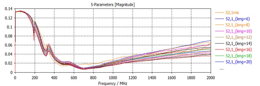
2.12 Comparison of Zlongitudinal from analytical derivation, theory
     and CST simulation. . . . . . . . . . . . . . . . . . . . . . . .      36
2.13 The model of the lossy rectangular pipe. . . . . . . . . . . . .       37
2.14 G versus a/b: it should be noted that G also includes the case
     of circular and square cross section, where it is equal to one.
     While, for values of a much larger than b, G tends to the case
     of a flat chamber. . . . . . . . . . . . . . . . . . . . . . . . . .   39
2.15 Ratio between the longitudinal impedance from simulation
     and the well-known from theory. In the case of: F=1, G=1.07
     and a = 3b . . . . . . . . . . . . . . . . . . . . . . . . . . . .     40
2.16 Ratio between the longitudinal impedance from simulation
     and the well-known from theory. In the case of: F=1, G=1
     and a = b . . . . . . . . . . . . . . . . . . . . . . . . . . . . .    40
2.17 Ratio between the longitudinal impedance from simulation
     and the well-known from theory. In the case of: F=0.93,
     G=1.114 and a = 1.5b . . . . . . . . . . . . . . . . . . . . . .       41
2.18 The elliptical pipe with half-height b,half-width a and length L.      42
2.19 The octagonal pipe with length L. The cross section is a reg-
     ular octagon, the width is equal to the height. . . . . . . . . .      43
2.20 Ratio between the longitudinal impedance from simulation
     and the well-known from theory. In the case of: F=0.99,
     G=1.04 and a = 4b . . . . . . . . . . . . . . . . . . . . . . . .      44
2.21 Ratio between the longitudinal impedance from simulation
     and the well-known from theory. In the case of: F=0.94,
     G=1.11 and a = 1.5b . . . . . . . . . . . . . . . . . . . . . . .      44
2.22 Ratio between the longitudinal impedance from simulation
     and the well-known from theory. In the case of F=0.93348,
     G=1 and l=41.30 mm. . . . . . . . . . . . . . . . . . . . . . .        45

3.1   Physical locations of the SPS kickers (red dots). Courtesy of
      M.Barnes . . . . . . . . . . . . . . . . . . . . . . . . . . . .   . 49
3.2   3D model of the MKP-L kicker: PEC material in grey, ferrite
      block in cyan, vaccum chamber in azure. . . . . . . . . . . .      . 50
3.3   Schematic model and setup: the central block is the MKP-
      L with the streched wire inside; on the sides, symmetrically,
      there is a block that represents a resistance circuit and one
      that represents a N-type connector. The whole is closed on
      two ports that represent the ports of the VNA. . . . . . . .       . 51
3.4   Model of a coaxial cable of length l, inner conductor of radius
      a and outer conductor of radius b. The insulating material
      with dielectric constant  and magnetic permeability µ. . . .      . 52

                                   4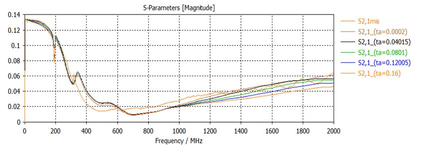
3.5  Equivalent circuit of a resistance . . . . . . . . . . . . . . . . .   53
3.6  Magnitude of S21 . In red the S21 from bench measurements,
     in green the simulated S21 related to the ideal circuit of the
     resistance and in blue the simulated S21 related to the real
     circuit of the resistance with the parasitic components (C =
     0.2 pF; L = 1 nH). . . . . . . . . . . . . . . . . . . . . . . . .     54
3.7 Relative percentage error. In blue the error experienced adopt-
     ing the real circuit of the resistance and in green adopting the
     ideal circuit of the resistance. (C = 0.2 pF; L = 1 nH). . . . .       55
3.8 Magnitude of S21 by varing the length of the coaxial cable. In
     orange the S21 from bench measurements. . . . . . . . . . . .          56
3.9 Magnitude of S21 by varing the dielectric constant of the PTFE.
     In orange the measured S21 . . . . . . . . . . . . . . . . . . .       56
3.10 Magnitude of S21 by varing the tangent loss of the PTFE. In
     orange the S21 from bench measurements. . . . . . . . . . . .          57

                                    5
I never see what has been done;
    I only see what remains to be done.
                           Marie Curie

6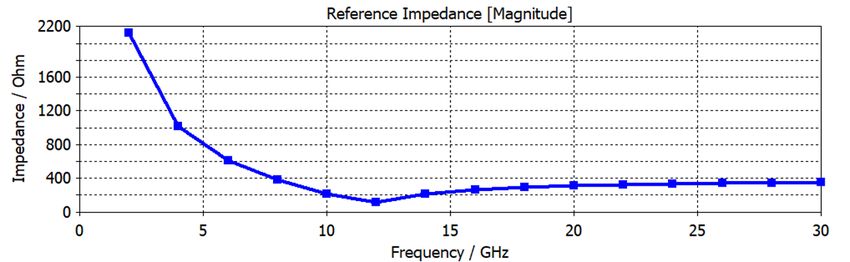
Acknowledgments

Poco più di un anno fa, mi sono rivolta al Prof. Andrea Mostacci esprimendo
il desiderio di voler svolgere un periodo di studio all’estero. Come risultato,
mi sono trovata in un paese al confine tra la Francia e la Svizzera per un corso
intensivo sulla scienza degli acceleratori di particelle. In altre parole, un mese
di studio matto e disperato nel quale ho scoperto l’affascinante mondo degli
acceleratori di particelle. E cosı̀ è nato il mio lavoro di tesi al CERN.
Ringrazio molto il Prof. per questo, e per la sua infinita gentilezza. Grazie
al Prof. Mauro Migliorati per la disponibilità e i consigli.

Un doveroso ringraziamento va al mio supervisor al CERN, il Dr. Carlo
Zannini, per la sua pazienza senza fine e per essere stato una grande guida
per la buona riuscita di questo progetto di ricerca.

I would like to thank my CERN section leaders, Elias Metral and Giovanni
Rumolo for giving me the opportunity to work in such a great team.

Un grande grazie va a tutta la mia famiglia e a chi mi è sempre accanto.
Grazie a mio fratello e in particolare ai miei nonni e ai miei genitori per il
profondo sostegno. L’opportunità più grande mi è stata donata da loro.

Grazie ad Alessandro, Francesca e Gianmarco, miei colleghi e amici, per
aver reso questi due anni di vita universitaria indimenticabili.

Grazie a Marco che è sempre con me.

                                                                  Alla prossima,
                                                                         Chiara

                                        7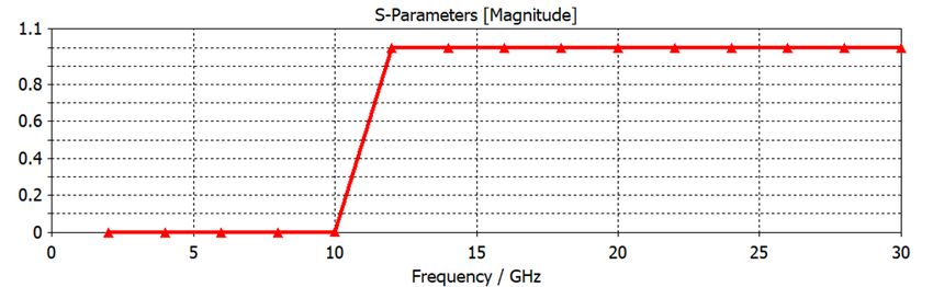
Introduction
An accurate computation of the beam coupling impedance is essential to
identify the accelerator structures causing performance limitations and im-
plement mitigation strategies.
    Ideally, the beam coupling impedance of a device should be evaluated by
exciting the device with the beam itself. However, in most cases, this solution
is not possible, and one must resort to alternative methods to consider the
effect of the beam.
    A well-established technique is to simulate the beam by a current pulse
flowing through a wire stretched along the beam axis. For beam coupling
impedance evaluations, the stretched wire method is a common and appre-
ciated choice. Nevertheless, the results obtained from wire measurements
might not entirely represent the solution of our initial problem, because the
presence of the stretched wire perturbs the EM boundary conditions. The
most evident consequence of the presence of another conductive medium in
the centre of the device under study is the fact that it artificially allows TEM
propagation through the device, with zero cut-off frequency. The presence of
a TEM mode among the solutions of the EM problem will have the undesired
effect to cause additional losses.
    The simulation of the beam coupling impedance of complex or rounded-
shaped accelerator elements is very challenging and frequency domain simu-
lations are more suitable for this kind of calculations, since a discretization
of the geometry with tetrahedral mesh cells is available, contrary to the time
domain case.
    The goal of this project is to investigate simulation methods in the fre-
quency domain to obtain the beam coupling impedance of arbitrary cross
section geometries without modifications of the device under test (stretched
wire, perturbing objects, etc.).
    In this framework, we identified a method to obtain the resistive wall
beam coupling impedance of arbitrary cross section geometries directly from
the scattering parameters, without modifications of the device under test.
This very promising method could pave the way to develop a measurement
technique to obtain the beam coupling impedance of vacuum chambers above
the pipe cut-off frequency without perturbing objects.
    We also addressed the benchmark of measurement setup of the model of
complex accelerator elements, with frequency domain simulations, by com-
paring the simulated and actual stretched wire measurements results. Here
we studied the case of the SPS injection kicker (MKP-L), looking carefully
at the correct representation of the termination of the stretched wire setup.
A very accurate representation of these terminations is crucial for the direct

                                       8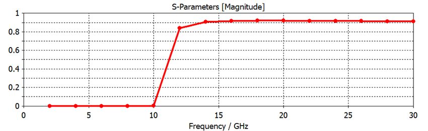
benchmark with bench impedance measurements.

                                 9
Chapter 1
The beam coupling impedance
A beam of charged particles flowing around an accelerator is affected, at low
intensity, by the Lorentz force produced by the “external” electromagnetic
fields generated by the the guiding and focusing magnets, RF cavities and
the other significant accelerator devices.
When the beam intensity increases, the beam can no longer be treated as a
collection of non-interacting single particles; indeed in addition to the “single-
particle phenomena”, “collective effects” become significant.
The term ”collective effects” refers to the set of phenomena in which the
evolution of the beam depends on the combination of external fields and
interaction between beam particles. These effects can be classified depending
on the type of interaction:
• space charge effects due to the Coulomb interaction between beam
particles
• wake fields effects caused by the interaction of the beam with its
surrounding
• beam-beam effects due to interaction of the beam with the contra-
rotating beam in a collider
• electron cloud effects due to the interaction between beam and elec-
trons produced in the accelerator structure
A very important issue for particle accelerators is produced by all these per-
turbations in both longitudinal and transverse plane. In particular, in this
thesis the attention is focused on the Fourier transform of the wake field,
the beam coupling impedance. In the ultra-relativistic limit, the causality
principle dictates that there can be no electromagnetic field in front of the
beam, which justifies the term “wake”.
10In more detail, a beam traveling inside a complex vacuum chamber, induces
charges and currents in the surrounding structures, which create electromag-
netic fields, precisely called wake fields. This e.m fields generated by the
head of the particle beam affect the tail itself and the beam motion causing
beam dynamics instabilities. As a consequence, an accelerator can be consid-
ered as a feedback device, where any longitudinal or transverse perturbation
occurring in the beam distribution may be amplified or damped by the e.m.
forces generated by the perturbation itself.
The impact becomes crucial when the beam intensity inside an accelerator
reaches higher values, in fact the beam motion is triggered and allowed to
grow, and without any damping mechanism, the beam is quickly degraded
or even lost.
Furthermore, the energy lost by the beam is eventually deposited as heat in
the accelerators devices, potentially causing damages.
Wake fields and the related impedance are usually responsible for tune shift,
emittance growth, beam loss and extra heating.
As the beam intensity increases, all these “perturbations” and their under-
lying mechanisms, should be properly quantified, studying the motion of the
charged particles, using the total electromagnetic fields, which are the sum
of the external and perturbation fields. The beam instabilities have been
the subjects of intense research for several decades. As the machines per-
formance was pushed new mechanisms were discovered and nowadays the
challenge consists in studying the interplays between all these phenomena,
since in most cases is not possible to treat the different effects separately.
In the specific case, studying the impedance is an essential part in the de-
sign phase of any accelerator, since it allows identifying possible mitigation
techniques, ensuring beam stability during operations and reducing beam
induced heating.
If possible or needed, the impedance should be kept as small as possible
without compromising the device functionality.
Fortunately, stabilising mechanisms are known, such as Landau damping,
electronic feedback systems and linear coupling between the transverse planes.
111.1 Theory of the beam-wall interaction
In this first chapter, the theory of the beam-wall interaction is described
by means of the concept of wake fields and beam coupling impedance, giv-
ing their physical meaning and mathematical treatment. The theoretical
analyses, computer simulations, and experimental measurements of these
quantities are crucial tasks in accelerator research. In the last part of the
chapter are mentioned some simulation methods to compute the beam cou-
pling impedance and is described a standard measurement technique and its
limitations.
1.1.1 Wake functions and beam coupling impedance
When the beam is traveling in a smooth and perfectly conducting pipe in-
duces a ring of negative charges, with the same velocity of the beam particles,
on the walls of the beam pipe, where the electric field ends, and these in-
duced charges create the so-called “image”, or induced current. However, if
the wall of the beam pipe is not perfectly conducting or contains geometry
variations, the movement of the induced charges will be slowed down, thus
leaving electromagnetic fields, which are proportional to the beam intensity,
mainly behind, called wake fields.
Figure 1.1: Relevant coordinates system: source particle q1 and test particle
q.
12In Fig. 1.1 there is a source particle q1 (z1 , r1 ) and a test particle q(z, r)
traveling with constant velocity v = βc, where c is the speed of light in
vacuum and β is the relativistic factor. The electromagnetic fields E and
B produced by the charge q1 in the structure can be derived by solving the
Maxwell equations imposing the proper boundary conditions. The Lorentz
force generated by the source particle q1 and acting on the test particle q is:
F = q[E + v × B] = q[Ez ẑ + (Ex − vBy )x̂ + (Ey + vBx )ŷ] = F|| + F⊥ . (1.1)
The Lorentz force is composed by the sum of two components, F|| is the
longitudinal force which changes the energy of the test particle and F⊥ is the
transverse force which deflects its trajectory.
The computation of these wake fields is quite challenging and two fundamen-
tal approximations are introduced:
• the rigid-beam approximation: the beam traverses a piece of equipment
rigidly, i.e. the wake field perturbation does not affect the motion of
the beam during the traversal of the impedance. The distance z of the
test particle behind some source particle does not change.
• the impulse approximation: as the test particle moves at the fixed
velocity v = βc through the accelerator component, can be considered
the impulse instead of the force point by point.
The energy variation is defined as the integrated longitudinal force acting on
the test particle along the structure. Considering a device of length L, it is
expresses as follows:
Z L
U (r1 , r) = F|| ds u U (z). (1.2)
0
The transverse deflecting kick includes the dipole kick and quadrupolar kick.
The first one is described by the following:
Z L
Mdip (r1 , r, z) = F⊥ |r=0 ds, (1.3)
0
that is the integrated transverse force from an offset source acting on a on-
axis test particle, while the quadrupolar kick is defined as the integrated
transverse force from an on-axis source acting on an offset test particle:
Z L
Mquad (r1 , r, z) = F⊥ |r1 =0 ds. (1.4)
0
13The longitudinal wake function is the energy loss normalized by the two
charges of the particles:
U (z)
w|| (z) = − [V /C] (1.5)
q1 q
The longitudinal wake function (Eq. (1.5)) does not depend on the transverse
positions. In the case of axisymmetric structures, in particular of cylindrical
symmetry and ultra-relativistic charges, the wake function can be expanded
in multipolar terms. In the longitudinal case, the dominant term is the first
one and the wake function depends only on z [2]. The minus sign in Eq. (1.5)
means that, for a positive wake, the test particle is losing energy.
It is important to introduce also the loss factor as follows:
U (z = 0)
k=− , (1.6)
q12
that is the energy lost by the source particle per unit charge squared.
From the above definitions we easily note that, when the charges travel on
the same trajectory, the loss factor is the wake function in the limit of zero
distance between q1 and q: k = wz (0). This is true in the case of β < 1,
while, in the relevant case β = 1 is valid the beam loading theorem, that
states:
w|| (z → 0− )
k= (1.7)
2
It means that an ultra-relativistic particle can only see half of its own wake
and it exists only in the region z < 0.
The energy lost by the source can be related to two components, the electro-
magnetic energy of modes that propagate down the beam chamber (above
cut-off), which will be eventually lost on surrounding lossy materials, and the
electromagnetic energy of the modes that remain trapped in the accelerator
devices. In the latter, this energy can be dissipated on the lossy walls or
it keeps ringing without damping, but can also be transferred to following
particles with the probability to feed into an instability.
Furthermore, also the transverse wake function Eqs. (1.8),(1.9) can be de-
fined, it is the transverse kick normalized by the two charges, in both the
case of dipolar and quadrupolar kick.
dip Mdip (z)
w⊥ = (1.8)
q1 q
quad Mquad (z)
w⊥ = (1.9)
q1 q
14A positive transverse wake means a defocusing transverse force. Similarly to
the longitudinal, the transverse wake functions can be expanded into a power
series in the offset of source and test particle [2]. Since no transverse effects
can appear when source and test particle are in the center of symmetry, the
zeroth order term of the power series is null.
Also in the transverse case, the wake vanishes for z > 0 due to the ultra-
relativistic approximation.
In the frequency domain, can be defined the analogous of the wake functions,
by performing its Fourier transform:
1 +∞
Z
ωz
Z|| = w|| (z)ej c dz, (1.10)
c −∞
the Eq. (1.10) is the expression of the longitudinal coupling impedance mea-
sured in Ohms. Here j is the imaginary unit and ω = 2πf is the angular
frequency.
The transverse impedance can be similarly defined by Eqs. (1.11),(1.12):
j +∞ dip
Z
dip ωz
Z⊥ = − w⊥ (z)ej c dz, (1.11)
c −∞
Z +∞
j ωz
Z⊥quad =− quad
w⊥ (z)ej c dz. (1.12)
c −∞
In general, the beam coupling impedance is a complex quantity: Z(ω) =
Zr (ω) + jZi (ω). Where, for the longitudinal impedance Zr (ω), Zi (ω) are
even and odd functions of ω, while for the transverse is the opposite.
151.1.2 Wake potential
The wake function defined in Eq. (1.5), is a Green function since it is gen-
erated by a point charge. When there is a bunch of particles moving on a
trajectory parallel to the axis, at a distance r1 , its wakefields can still be
computed from the wake function of the point charge for any bunch dis-
tribution. Indeed, considering, for example, the longitudinal plane and a
bunch with longitudinal distribution λ(z), the wake function produced by
the bunch distribution at a point z, is simply given by the convolution of the
Green function over the bunch distribution. In practice, the convolution in-
tegral is obtained by applying the superposition principle. The distribution
is splitted into an infinite number of infinitesimal slices summing up their
wake contributions at the point z 0 (see Fig. 1.2).
Figure 1.2: At the top the Bunch spatial distribution. In the center the slice
view if the bunch. At the bottom the wake left behind each slice.
16According to the definitions given so far, wake potential of a bunch is ex-
pressed as follows:
1 z
Z
W|| (z) = w|| (z 0 − z)λ(z 0 )dz 0 (1.13)
Q −∞
where Q is the total charge of the bunch.
The same consideration can be done for the transverse plane, the transverse
wake potential is:
1 z
Z
W⊥ (z) = w⊥ (z 0 − z)λ(z 0 )dz 0 (1.14)
Q −∞
1.1.3 Relationship between longitudinal and transverse
impedance
Since the particles move at the fixed velocity v = βc through the accelerating
structure, an important quantity is the impulse, defined as follows:
Z +∞ Z +∞
∆p(x, y, z) = Fdt = q[E + v × B]dt (1.15)
−∞ −∞
From the definition of the impulse can be introduced an important theorem
which links the transverse and longitudinal impedance.
Starting from the four Maxwell equations, for a particle in the beam, can be
shown (considering β = 1):
∇ × ∆p(x, y, z) = 0 (1.16)
which is known as Panofsky-Wenzel theorem [3]. This relation is very general,
as no boundary conditions have been imposed. With some mathematical pas-
sages, it can be shown that a consequence of the Panofsky- Wenzel theorem
is the following relationship:
∂
∇⊥ w|| (z) = w⊥ , (1.17)
∂z
The Eq. (1.17) can link the longitudinal with the dipole transverse impedance
by performing the Fourier transform.
171.2 Simulations and measurements
For each particle accelerator design, the careful establishment of an impedance
budget is a prerequisite for reaching desired performances. Therefore, the-
oretical analyses, computer simulations, and experimental measurements of
the beam coupling impedance of accelerator components are critical tasks
in accelerator research, design, and development. Concerning the computer
simulations, can be sorted into three main groups, namely Time Domain
(TD), Frequency Domain (FD), and methods without a particle beam. The
most common are TD methods, since they require only matrix-vector mul-
tiplications for time stepping. They are usually based on finite differences
time domain (FDTD, Yee 1966 [4]) or finite integration technique (FIT, Wei-
land 1977 [5]),which result in a coinciding space discretization on a Cartesian
mesh.
TD simulations are suitable at medium and high frequency, and particularly
in perfectly conducting structures. They are unfavourable for low frequencies
and low velocity of the beam. Also, dispersively lossy materials are difficult
to treat in TD, since a convolution with the impulse response, i.e. the inverse
Fourier transform (FT) of the material dispersion curve, is required. In FD
the beam velocity and dispersive material data are just parameters. How-
ever, a system of linear equations (SLE) has to be solved for each frequency
point, which is costly when the matrix is large and ill-conditioned. The most
common method without particle beam is the computation of eigenmodes,
which can be related to the wake function as discussed in [6]. Other methods
that involve different excitations from particle beam are describes in [8], [9],
[10], but they require special interpretations to obtain the beam coupling
impedance.
The most common software used is CST Studio Suite [11], a 3D electromag-
netic Computer Aided Design (CAD) tool, widely used for the computation
of wakes and impedances.
In particular, the Wakefield solver of Particle Studio (PS) solves Maxwell’s
equations in time domain, using a particle bunch as excitation of the struc-
ture under study. The outputs of the simulation are the wake potential and
the beam coupling impedance. The wake function is produced by the ex-
citing Gaussian bunch, that is the source, as a function of the time delay τ
with respect to the passage of the source. It is the the voltage gain of a unit
charge crossing the structure with a delay τ with respect to to the leading
charge, due to the fields created by the latter. The beam coupling impedance
is its Fourier transform normalized to the bunch spectrum, in other words
the equivalent of the wake potential in the frequency domain.
Concerning the experimental measurements, ideally, the evaluation of the
18beam coupling impedance of the accelerator components should be performed
by exciting the device with the beam itself. However, this method, which
in principle is the best one, is not always possible. In addition, when we
need information on the behaviour of the components before the set up of
the machine, it is desiderable to perform bench measurements.
For this purpose, the stretched Wire method (WM) [2] is a common choice
to establish the beam coupling impedance of accelerator structures in mea-
surement. The WM is also a common approach used in frequency domain
simulations to approximate the beam excitation.
1.2.1 The Wire method and its limitations
The Wire method was proposed in the first half of the 70’s, based on in-
tuitive considerations. There has been a long history in the development
of this method and in the improvement of its accuracy, in both theory and
technique [12],[13]. Today it is widely used, at CERN the method was em-
ployed already in the second half of the 70’s to measure the longitudinal and
transverse beam coupling impedance of a kicker in the frequency domain
[14]. Furthermore, an improved version of the bench measurement technique
of the Wire method was proposed by V. G. Vaccaro [2].
The intuitive consideration on which the method is based is that the particle
beam can be replaced by a current pulse with the same temporal behaviour
of that associated to the beam, but flowing through thin metallic wire placed
along the beam axis.
Figure 1.3: Thin metallic wire placed along the beam axis of a structure.
An accelerator component with a thin metallic wire on its beam axis can
19be considered as a two-port circuit, which can be characterized with a Net-
work Analyzer. In particular, the transmission scattering parameters of the
Device Under Test (DUT) and the reference beam pipe (REF) can be mea-
sured. The longitudinal beam coupling impedance of the DUT can be found
as follows [15]:
S21REF
Zlongitudinal = Z|| = 2Zch −1 , (1.18)
S21DU T
Zch is the characteristic impedance of the equivalent transmission line formed
by the wire and the DUT wall.
In 1993, Vaccaro [2] derived a more rigorous and accurate formula, based
on the transmission line theory. He showed that the longitudinal coupling
impedance in a transmission line (see Fig. 1.4) can be expressed by:
2 2 l
Z|| = jZch (kDU T − kR ) (1.19)
kREF
Figure 1.4: Transmission line equivalent circuit for a DUT. The (Ro + jωLo )
1
and jωC o
are the distributed parameters per unit length which form the Zch ;
Z|| and l are the longitudinal impedance and length of the DUT, respectively.
The kDU T and kREF are the propagation constant of the DUT and REF.
Since the transmission line is symmetrical, the related scattering matrix is
20the Eq. (1.20):
2
(Zch − Zr2 ) sin kl −2jZr Zch
2
−2jZr Zch Zch − Zr2 ) sin kl
S= 2
(1.20)
(Zch + Zr2 ) sin kl − 2jZr Zch cos kl
where Zr is a reference impedance.
If the line is matched implies S11 = S22 = 0 and Zr = Zch and in addition
the propagation constant can be related to transmission coefficient by Eq.
(1.21):
S21 = exp (−jkl), (1.21)
and the longitudinal coupling impedance can be expressed as in Eq. (1.22).
S21DU T ln S21DU T
Z|| = −Zch ln 1+ . (1.22)
S21REF ln S21REF
In most cases of the accelerator components, the S21DU T is close to S21REF
and the formula can be approximated by the well-known Log-formula of Eq.
(1.23)
S21DU T
Z|| = −2 · Zch ln . (1.23)
S21REF
The Wire Method for Coupling Impedance evaluations is quite appealing
for the possibility to make bench measurements and to simulate the beam
excitation in frequency domain, indeed the scattering parameters as well
as the characteristic impedance are direct outputs of the simulations and
measurements. Neverthless, this established method has some limitations
due to the presence of the wire that perturbs the electromagnetic boundary
conditions. In fact, the conductor in the center of the structure modifies its
cross section that is no longer simply connected, and artificially allows the
propagation of TEM modes with zero cut-off frequency. Therefore, the WM
might not entirely represent the solution of our initial problem leading to
additional losses during the measurements.
21Part I
A new method to obtain the
Beam Coupling
Impedance from Scattering
parameters
22Chapter 2
A new approach to compute
the beam coupling impedance
In the previous chapter, a brief overview of the methods to compute the
beam coupling impedance focusing on the wire method, with its principle
of operation and theoretical bases, have been discussed. Furthermore, the
limitations of the method have been also presented. In this section, a new
method to asses the longitudinal beam coupling impedance of the accelerator
components, which does not require the modification of the DUT, has been
introduced.
The new formula relating the longitudinal beam coupling impedance and the
scattering parameters has been analytically validated for a resistive circular
chamber. The generalization to arbitrary chamber shapes has also been
discussed. Furthermore, the related simulation method is described together
with its main simulation settings.
2.1 From the Wire Method to a new formula
Although the Wire method is a well established technique in the world of
particle accelerators, the study of its limitations and the development of new
methods that overcome these limitations is a high demand task. In this
regard, to exceed the issues explained in the subsection 1.2.1, the attention
has been focused to possible approaches without modification of the DUT.
The longitudinal beam coupling impedance is essential related to the energy
loss of the electromagnetic wave propagating in the structure and, therefore,
is intrinsically linked to the transmission scattering parameter. Given these
considerations and the fact that there are no obvious contradictions, the
intuition has led to study the first propagating TM mode of the DUT, instead
23of the TEM of the equivalent transmission line formed by the wire and the
conductive wall in the case of the WM.
The proposed relation to evaluate the impedance without modifications of
the device under test has the following form (Eq. (2.1)):
|S21DU T |
Zlongitudinal = −K · Zmode ln . (2.1)
|S21REF |
The expression is quite similar to the Log-formula, where the characteristic
impedance of the equivalent transmission line is replaced by the appropri-
ate impedance of the propagating mode. The S21DU T refers to the Device
Under Test, that is the structure with finite electric conductive walls, while
the S21REF refers to the same structure with Perfect Electric Conductive
(PEC) walls. The reference scattering parameter has been involved in order
to obtain an accurate evaluation of the impedance even under the cut-off
frequency of the pipe. Furthermore, the S21 and the Zmode refer to the first
TM propagating mode. The term K is a constant.
2.2 Analytical validation of the proposed for-
mula
The circular resistive structure under test is displayed in Fig. 2.1, where b is
the pipe radius, L is the pipe length and σ = 3000 S/m the wall conductivity.
Figure 2.1: Model of the lossy circular pipe.
The longitudinal beam coupling impedance of the circular resistive pipe can
be analytically calculated by using the following well-known equation [16]:
theory L
Zlongitudinal = ζ, (2.2)
2πb
24where ζc is the wall surface impedance, and for simplicitypin the thick wall
regime and for good conductors ζc = (1 + j)ζ, with ζ = ωµ 2σ
0
; ω = 2πf is
the angular frequency, µ0 the magnetic permittivity of free space.
In order to validate the proposed approach is necessary to demonstrate that
the formula of Eq. (2.1) reduces to the theoretical formula of Eq. (2.2), it
means:
−K · Zmode · ln |S21DU T |
|S21REF |
→ ζc
2πb
L.
As a first step, the analytical expression of the S21 of the lossy circular pipe
is derived from [17], where an expression of the attenuation constant α of
the lossy circular waveguide is obtained, applying the Leontovich boundary
condition:
s
1 jk 2 ( unm )2
α = Im k02 − 2 [unm + unm 03 µ0b ], [1/m], (2.3)
b ω( b ) ( ζc + 0 ζc )
The S21 parameter can be computed from the equation of conservation of
the energy:
|S11 |2 + |S21 |2 = 1 − α0 , (2.4)
assuming |S11 | = 0: √
|S21 | = 1 − α0 . (2.5)
The term α0 refers to the adimensional losses, and can be derived from Eq.
(2.3) as follows:
α0 = 1 − e−2|α|z , (2.6)
so it turns out: √
|S21 | = e−2|α|z = e−|α|z . (2.7)
Therefore, to benchmark the analytical derivations with simulations, a com-
parison is displayed in Figs. 2.2, 2.3.
25Figure 2.2: Comparison between α. In green α obtained from simulations
and in red α evaluated from theoretical computations
Figure 2.3: Comparison of S21. In red S21 obtained from simulations and in
blu S21 evaluated from theoretical computations
The plots show that there is a perfect agreement between the two approaches.
Therefore Eq. (2.1) can be computed by using the S21 of Eq. (2.7), so it is:
ln |S21 | = −|α|z. (2.8)
26The derivation of the α is detailed in the Appendix A.
The attenuation constants below and above pipe cut-off frequency can be
expressed as follows: 1 :
r
4 u2 ζ ζ
αbelow cut−of f = − (k02 − 2 + 2ω0 )2 + (−2ω0 )2 (2.9)
b b b
r
4 u2 ζ ζ −ω0 ζ
αabove cut−of f = (k02 − 2 + 2ω0 )2 + (−2ω0 )2 ( 2 u2 b ).
b b b k0 − b2 + 2ω0 ζb
(2.10)
Calculation of the beam coupling impedance below pipe cut-off
frequency
For the lossy circular pipe the attenuation called αDU T can be written as in
Eq.(2.9).
For the reference PEC pipe the attenuation is written as follows:
r
u2
αREF = −Im[ (k02 − 2 )], (2.11)
b
The longitudinal impedance is then derived from Eq.(2.1) and applying the
relation of Eq.(2.8):
|S21DU T |
ln = ln (e(|αREF |−|αDU T |)L ) = (|αREF | − |αDU T |)L (2.12)
|S21REF |
and considering the full
q
expression of the longitudinal impedance (Eq.(2.1))
2
(k02 − u2 )
and Zmode = ZT M = ω0
b
:
Zlongitudinal =
q
u2
(k02 − )
r r
u 2 u2 ζ ζ
b2 4
−K · Im (k02 − 2 ) − (k02 − 2 + 2ω0 )2 + (2ω0 )2 L
ω0 b b b b
(2.13)
It can be shown, with some mathematical manipulations, that the longi-
tudinal impedance obtained from the analytical approach (Eq.(2.13)) has
the same expression of the theoretical impedance (Eq.(2.2)).
1
The expression of α is different below and above cut off frequency, see Appendix A
27Zlongitudinal =
q
u2
(k02 − )
r r
b2 u2 u2 ζ 2 HH ζ 2
4
= −K · k02 − 2 −
+ (2ω 0 )) + (2ωH (k02 −
0 H) L
ω0 b2 b b bH
(2.14)
ζ 2
The term (2ω0 b ) can be neglected when the structure can be treated as a
planar geometry, that is:
r
2 1
b >> δ = → f >> (2.15)
ωµ0 σ πσµ0 b2
Under this condition, Eq.(2.14) reduces to:
q
2
r
(k02 − u2 ) (2ω0 ζb )
q
u2 u2
= −K · ω0
b
k0 − b2 − 4 [(k02 −
2
b2
)(1 + 2 )]2 L =
(k02 − u2 )
b
q
2
r
(k02 − u2 ) (2ω0 ζb ) 2
q q
u2 u2
= −K · ω0
b
k02 − b2
− k02 − b2
4
(1 + 2 ) L=
(k02 − u2 )
b
q
u2
(k02 − )
r
b2 u2 (2ω0 ζb ) 1/2
= −K · k02 − 2 · (1 − (1 + 2 u2 ) ) L (2.16)
ω0 b (k0 − b2 )
(2ω0 ζb ) (2ω0 ζb )2 (2ω0 ζb )
The term 2 is small, 2Calculation of the beam coupling impedance above pipe cut-off
frequency
For the lossy circular pipe the attenuation called αDU T can be written as in
Eq.(2.10).
For the reference PEC pipe the attenuation is written as follows:
αREF = 0, 2 (2.20)
The longitudinal impedance is then derived from Eq.(2.1) and applying the
relation of Eq.(2.8):
|S21DU T |
ln = ln (e(|αREF |−|αDU T |)L ) = (−|αDU T |)L (2.21)
|S21REF |
and considering the full
q
expression of the longitudinal impedance (Eq.(2.1))
2
(k02 − u2 )
and Zmode = ZT M = ω0
b
:
Zlongitudinal =
q
u2
(k02 − )
r
b2 4 u2 ζ 2 ζ 2 −ω0 ζb
−K · (k02 − 2
+ 2ω0 ) + (−2ω0 ) u2 ζ
L
ω0 b b b (k02 − b2 + 2ω0 b )
(2.22)
Above the cut-off frequency of the pipe, under the condition k02 >> 2ω0 ζb ,
it can be shown show that the longitudinal impedance obtained from the
analytical approach (Eq.(2.22)) has the same expression of the theoretical
impedance (Eq.(2.2)).
Indeed, under the same condition f >> πσµ10 b2 the Eq.(2.22) assumes the
following form:
q
2
(k02 − ub2 )2 4
r
2 u2 2 ω0 ζb ζ
Zlongitudinal = K · (k0 − 2 ) 2 u2 L = K L (2.23)
ω0 b (k0 − b2 ) b
For both cases below Eq. (2.19) and above Eq. (2.23) cut-off frequency
1
with K = 2π the expressions become exactly the well-known theoretical
longitudinal impedance.
2 u2
above cut off frequency (k02 − b2 ) > 0, so its imaginary part is zero: αREF =
q
2
Im[ (k02 − ub2 )] = 0 .
29q
The condition 3 b >> δ = ωµ20 σ → f >> πσµ10 b2 means that the radius of
curvature can be neglected and therefore also the attenuation caused by the
propagation of cylindrical waves.
For instance, in the present case, where the circular pipe has a wall electrical
conductivity σ = 3000 S/m and radius b = 10 mm, the condition results in
f >> 8.5 kHz. This means that the frequency range in which the equal-
ity (2.23) is valid, must be sufficiently above 8.5 kHz. In fact in the case
studied, the frequency range of interest is above 1 GHz, then the method
is valid. Furthermore, it is important to underline that, the frequency limit
of application of the method is indirectly proportional to the wall electrical
conductivity σ. As a consequence, for higher conductivity (pipe with less
losses) the frequency limit scales at lower frequencies while for lower conduc-
tivity (pipe with more losses) the limit is at higher frequencies.
The analytical validation asserts that the longitudinal beam coupling impedance
can be computed with the following formula:
ZT M |S21DU T |
Zlongitudinal = − ln (2.24)
2π |S21REF |
In Fig. 2.4 is displayed the impedance from the analytical derivation and the
impedance from the theory for a lossy circular pipe.
The perfect agreement between the impedances is evident below and above
the cut-off frequency of the pipe, while around the cut-off frequency is not
perfect, due to the analytical approach which does not provide an estimation
of the impedance at the cut-off frequency.
3
It is important to note that the imposed condition is not a real limitation of the
proposed formula, but a mathematical simplification to make the calculations simpler.
Indeed, the analytical formula derived for the impedance is much more general.
30Figure 2.4: Comparison between Zlongitudinal from the analytical computation
and theory.
2.3 Simulation method
In the previous paragraph, the analytical expressions of Zlongitudinal below
(Eq.(2.13)) and above (Eq.(2.22)) the cut-off frequency of the pipe have been
derived.
These equations have been obtained in the hypothesis that the beam coupling
impedance can be expressed from the scattering parameters as described in
Eq.(2.1). The equations have been shown to reduce exactly to the well-known
longitudinal impedance (Eq. (2.2)) for f >> πσµ10 b2 , proving the correctness
of the relation between the scattering parameter S21 and the longitudinal
beam coupling impedance proposed in Eq.(2.1).
At this point, the discussion of the new possible method to get the impedance
continues showing how this has been implemented in simulation. With this
aim, the simulation settings are shown referring to the circular pipe of Fig.
2.1.
First of all, in order to excite the structure, the Waveguide Ports are used
and displayed in Fig. 2.5.
This kind of Ports allow to set a specific number of modes to be simulated
and the frequency domain solver of CST computes the scattering parameters
for each mode set at the port.
31Figure 2.5: In red the Waveguide Port for circular pipe. In order to excite
the first TM mode at least three modes must to be set at the port.
The frequency domain solver is equipped with the tetrahedral mesh cells
that allow a better discretization of the calculus domain, contrary to the
time domain solver where hexahedral mesh cells are used..
From the Fig. 2.6 is clear the advantage of using the tetrahedral mesh cells,
especially for round geometries. Indeed, the aim of the proposed method is
also to establish an accurate procedure to compute the impedance of curved
and complex geometries.
Figure 2.6: Mesh view for a sphere in the case of hexahedral and tetrahedral
mesh cells.
In the example of Fig. 2.6 it can be observed that, using the same number
of mesh cells, the sphere is better represented in the case of tetrahedral
discretization.
32To determine the right number of tetrahedrons, the numerical convergence of
the simulation results versus the number of tetrahedrons has been studied. A
good compromise between computational time and accuracy of the simulation
results is shown in the figure 2.7.
The first studies are carried out by using the ”Discret Sample Only” method
of the frequency domain solver. The frequencies to be simulated are chosen
to explore the pipe behaviour below and above its cut-off frequency.
Figure 2.7: Mesh view: the pipe is discretized with 65373 tetrahedral mesh
cells (pipe radius= 10 mm, pipe length= 50 mm).
To perform the study of longitudinal impedance with new formula of Eq.
(2.24) the involved parameters to be considered are the mode impedance
and the transmission scattering parameter of the first TM propagating mode.
The following formula gives its cut-off frequency [19]:
u01 2.4048
fcT M 01 = c= c = 11.6 GHz (2.25)
2πb 2πb
where u01 = 2.4048 is the first zero of the Bessel J0 and c is the speed of light
in vacuum.
Furthermore, the S21 and ZT M are direct output of the simulation. They are
reported, for the specific pipe, in Figs. 2.8,2.9, 2.10.
33Concerning the S21DU T , above the cut-off frequency of the pipe (fc = 11.6
GHz), its value is below one due to the losses caused by the finite conductiv-
ity of the walls. Instead, the S21REF as expected, is just equal to one.
The same situation occurs also below the cut-off frequency, where both the
S21DU T and S21REF are affected by propagation losses, because the mode does
not propagate, and the S21DU T also by the losses due to the finite conductiv-
ity of the wall. The S21REF is essential to extrapolate the losses due to the
finite conductivity of the wall below the cut-off frequency of the pipe.
Figure 2.8: S21 of first TM mode of the Resistive Wall structure. The S21 is
plotted in linear magnitude.
Figure 2.9: S21 of first TM mode of the PEC wall Wall structure. The S21 is
plotted in linear magnitude.
34Figure 2.10: Real part of the impedance of first TM mode of the Resistive
Wall structure. The imaginary part is zero.
The formula (2.24) applied to this circular pipe gives the impedance in Fig.
2.11.
Figure 2.11: Zlongitudinal from simulation.
The longitudinal impedance computed from frequency domain simulations
by using Eq. (2.24) has been compared with the exact theoretical evaluation
and the analytical derivation in Fig. 2.12. A larger fluctuation is observed
below the cut-off frequency of the pipe that could be caused by numerical
errors due to the very small value of the transmission coefficient.
These results shows that, the proposed approach is a suitable and accurate
method to compute the beam coupling impedance through simulation stud-
ies.
35Figure 2.12: Comparison of Zlongitudinal from analytical derivation, theory
and CST simulation.
2.4 Generalization of the method to an arbi-
trary chamber cross section
In the previous paragraph has been identified with the associated analytical
validation, a method to obtain the RW beam coupling impedance of a circu-
lar chamber directly from the scattering parameters, without modifications
of the DUT. In this section, the generalization of the method to arbitrary
shapes of the vacuum chambers is explored. As a first step, the case of the
rectangular chamber is studied to investigate the applicability of the method
to non-axially symmetric structures. Therefore, the generalization to arbi-
trary shapes is tested for the case of elliptical and octagonal chambers.
2.4.1 Rectangular accelerators chamber
The generalization of the method is studied analytically on the rectangular
chamber of Fig. 2.13, with height 2b, width 2a, pipe length L and wall
electrical conductivity σ.
The goal of the analytical study is to figure out if the impedance can be
still obtained from the scattering parameters as expressed by the Eq. (2.24).
36Figure 2.13: The model of the lossy rectangular pipe.
As a first step, the analytical expression of the S21 of the lossy rectangular
pipe has been derived. The expression of S21 is obtained from the attenua-
tion constant α.
For a rectangular waveguide, an expression of α for TM mode is provided in
[20], applying the power loss method (PLM). This method assumes that the
expression of the fields, in a highly but imperfectly conducting waveguide,
is the same as those of a lossless waveguide. Neverthless, in literature it is
shown that, far above the cut-off frequency, the power loss method provides
a good approximation of α also in the imperfectly conducting waveguide.
Therefore, the aim of this approach is to determine the expression of Zlongitudinal
above cut-off, using the attenuation constant obtained with the simplified
method (PLM), and verify if the achieved expression can be used to evaluate
the longitudinal beam coupling impedance.
37It turns out 4 :
2ζ(m2 (2b)3 + n2 (2a)3 )
α= q , [1/m] (2.26)
η(2a)(2b) 1 − ( ffc )2 (m2 (2b)2 + n2 (2a)2 )
where m, n are integer indices and define the possible modes that propagates;
η is the intrinsic impedance of free space; fc is the pipe cut-off frequency and
b, a are the half-height and the half-width of the pipe, respectively.
In order to compute the impedance of Eq.(2.24), in the range above cut-off
frequency, it is necessary to evaluate the following parameters:
ln S21 = −|α|z, (2.27)
where for f >> fc , for T M11 mode and z = L, it is:
r
ω0 b3 + a3 1
ln S21 = − ·L (2.28)
2σ b2 + a2 ab
Now, the theoretical longitudinal impedance of rectangular pipe is the fol-
lowing:
rect circ ZTcirc
M
Zlongitudinal = F · Zlongitudinal = −F · ln |S21circ |, (2.29)
2π
where F is the Yokoya longitudinal form factor for rectangular pipe (see [21]),
which allows to obtain the longitudinal impedance of an arbitrary pipe cross
circ
section, with respect to the circular one. While, Zlongitudinal is the Eq. (2.24)
obtained in the previous chapter.
From Eqs. (2.10),(2.21) it is:
circ ζL
ln |S21 |=− , (2.30)
bZTcirc
M
so it can be written:
circ
ln |S21 | − bZζLTM
η
rect = p ω0 (b3 +a3) = G , (2.31)
ln |S21 | − 2σ b2 +a2 ab 1
·L ZTcirc
M
(b2 +a2 )a
where G = (b3 +a3 )
is a geometrical factor displayed in Fig. 2.14.
From the Eq. (2.31):
circ η rect
ln |S21 |=G ln |S21 | (2.32)
ZTcirc
M
4
This is the expression for TM modes
38Figure 2.14: G versus a/b: it should be noted that G also includes the case of
circular and square cross section, where it is equal to one. While, for values
of a much larger than b, G tends to the case of a flat chamber.
Then, substituting Eq.(2.32) in (2.29) it is:
rect G rect
Zlongitudinal =− ln |S21 |ηF (2.33)
2π
The analytical derivation shows that, also in the case of rectangular pipe,
the impedance can be derived from the scattering parameter S21 .
It is important to point out, that Eq.(2.33) was derived in the assumption of
being far above the cut-off frequency, where the impedance of the TM mode
tends to the impedance of the free space η 5 .
It means that, in the range above cut-off frequency, the longitudinal impedance
of a rectangular pipe can be expressed as follows:
rect G rect
Zlongitudinal = −F · ZT M ln |S21 |, (2.34)
2π
It is worth mentioning that Eq. (2.34) is a more general expression of Eq.
(2.24). In fact for a circular chamber F and G are equal to 1 and Eq. (2.34)
would reduce exactly to Eq (2.24).
Simulation tests are done to benchmark the longitudinal impedance of Eq.(2.34)
5
From the theory is easy to show that, far above the pipe cut-off frequency, it is:
ZT M = √ηr , where r is the relative dielectric constant of the medium in which the mode
is propagating. In this case the medium is the vacuum, then r = 1
39with the exact and well-known theoretical impedance of a rectangular cham-
ber of Eq. (2.35):
theory ζL
Zlongitudinal =F (2.35)
2πb
The goal is to demonstrate that Eq. (2.34) can be used to compute the
longitudinal impedance of rectangular chambers.
In Figs. 2.15, 2.16, 2.17 are displayed the ratio between the two impedances
for different values of a and b, in the range above the cut-off frequency.
Figure 2.15: Ratio between the longitudinal impedance from simulation and
the well-known from theory. In the case of: F=1, G=1.07 and a = 3b
Figure 2.16: Ratio between the longitudinal impedance from simulation and
the well-known from theory. In the case of: F=1, G=1 and a = b
40Figure 2.17: Ratio between the longitudinal impedance from simulation and
the well-known from theory. In the case of: F=0.93, G=1.114 and a = 1.5b
The case of a = 1.5b (see Fig. 2.17), is a clear proof of the importance of the
G factor. Indeed, the ratio is equal to one with a relative error less then 1%
and without the G factor it would be much higher, reaching the value of 11%.
It is evident that the Eq. (2.34) can be used to obtain the longitudinal beam
coupling impedance of rectangular chambers. A more general expression
valid for both circular and rectangular chamber can be written as follows:
ZT M |S21DU T |
Zlongitudinal = −F · G ln , (2.36)
2π |S21REF |
where ZT M always refers to the first TM propagating mode.
412.4.2 Elliptical and octagonal accelerators chamber
In the previous section a possible generalization has been demonstrated for
the case of a RW rectangular chamber in the range above the cut-off fre-
quency. The formula of the circular case (Eq. (2.24)) has been extended
to the rectangular by means of appropriate factors. These factors, in the
specific case, are the Yokoya form factor and the G factor. The G factor can
be defined as a geometrical factor related only to the width and height of the
geometry under test, which has been analytically derived. The equation in-
cluding these factors is more general and can be applied to both circular and
rectangular chamber (Eq. (2.36)). The intuition suggests that the method
could be extended to other more complex geometries as long as the half-
height and half-width of the cross section can be defined for these structures.
Consequently, in this section, the developed method is tested on RW cham-
ber with elliptical and octagonal cross section of Figs. 2.18, 2.19, with the
same simulation settings of the previous cases. Indeed, the simulations are
carried out with the frequency domain solver, using the Waveguide Port to
excite the structure and the tetrahedral mesh cells to discretize the model .
The studies are performed with the ”Discret Sample Only” method of the
frequency domain solver, exploring the pipe behavior below and above its
cut-off frequency.
Figure 2.18: The elliptical pipe with half-height b,half-width a and length L.
42Figure 2.19: The octagonal pipe with length L. The cross section is a regular
octagon, the width is equal to the height.
The approach consists, in testing the Eq.(2.36), on the elliptical and octag-
onal pipe.
2 2 )a
G = (bb3+a
+a3
is the geometrical factor reported in Fig. 2.14, that can be com-
puted also for the elliptical and octagonal case, considering the half-width a
and the half-height b of the cross section.
The longitudinal beam coupling impedance of the elliptical and octagonal
RW pipe can be analytically calculated from the circular one using the ap-
propriate form factor F (Eq. (2.35)). For the elliptical case, F is the already
known Yokoya longitudinal form factor (see [21]), and for the octagonal case
is computed with respect to a reference circular pipe with CST simulations
as could be done for any kind of shapes (see [22]). ζ is the wall impedance,
b the height and L the length of the pipe.
To apply this formula, the RW pipe must have the same conductivity, height
and length of the reference circular pipe.
The purpose is to benchmark the impedance obtained from simulations using
Eq.(2.36), with the theoretical impedance in (2.35).
43Elliptical RW pipe
The comparison between the impedances is provided by the following plots
(Figs. 2.20, 2.21), where is displayed the ratio between the simulated longi-
tudinal impedance and the theoretical one, above cut-off frequency.
The simulations are carried out for different elliptical cross sections of the
pipe, which means different value of a, b and then F and G.
The results show that the ratio is always one with a relative error less or
equal to 1%. In particular, for the case of a = 1.5b, is evident that without
the G factor the relative error would be much higher leading to an incorrect
impedance estimation.
Figure 2.20: Ratio between the longitudinal impedance from simulation and
the well-known from theory. In the case of: F=0.99, G=1.04 and a = 4b
Figure 2.21: Ratio between the longitudinal impedance from simulation and
the well-known from theory. In the case of: F=0.94, G=1.11 and a = 1.5b
44Octagonal RW pipe
The comparison between the impedances, also in the case of regular octagonal
cross section, is performed by plotting the ratio between the two in Fig. 2.22.
Figure 2.22: Ratio between the longitudinal impedance from simulation and
the well-known from theory. In the case of F=0.93348, G=1 and l=41.30
mm.
The result proves that also in the case of octagonal chamber the impedances
agree, indeed the ratio is equal to one with a relative error less than 1 %.
These simulation tests suggest that Eq. (2.36) is a general expression that
could be applied to obtain the longitudinal beam coupling impedance of
arbitrary shaped chambers.
45You can also read