Influence of survival, promotion, and growth on pattern formation in zebrafish skin - Nature
←
→
Page content transcription
If your browser does not render page correctly, please read the page content below

www.nature.com/scientificreports
OPEN Influence of survival, promotion,
and growth on pattern formation
in zebrafish skin
Christopher Konow1, Ziyao Li1, Samantha Shepherd1,2, Domenico Bullara1 &
Irving R. Epstein1*
The coloring of zebrafish skin is often used as a model system to study biological pattern formation.
However, the small number and lack of movement of chromatophores defies traditional Turing-type
pattern generating mechanisms. Recent models invoke discrete short-range competition and long-
range promotion between different pigment cells as an alternative to a reaction-diffusion scheme.
In this work, we propose a lattice-based “Survival model,” which is inspired by recent experimental
findings on the nature of long-range chromatophore interactions. The Survival model produces
stationary patterns with diffuse stripes and undergoes a Turing instability. We also examine the
effect that domain growth, ubiquitous in biological systems, has on the patterns in both the Survival
model and an earlier “Promotion” model. In both cases, domain growth alone is capable of orienting
Turing patterns above a threshold wavelength and can reorient the stripes in ablated cells, though
the wavelength for which the patterns orient is much larger for the Survival model. While the Survival
model is a simplified representation of the multifaceted interactions between pigment cells, it reveals
complex organizational behavior and may help to guide future studies.
Morphogenesis, the symmetry-breaking phenomenon in which a uniform mass (such as an embryo) spontane-
ously develops complex yet organized heterogeneities in a reproducible manner1,2, has fascinated biologists and
mathematicians for decades. One influential theory of morphogenesis, developed by Alan T uring1, explains how
a simple two-morphogen reaction-diffusion system can spontaneously develop spatially periodic, temporally
stationary structures. Gierer and Meinhardt later rederived and expanded on this idea, emphasizing the concept
of short-range activation and long-range inhibition (SRALRI), whereby an activator is able to locally increase
its concentration (usually in an autocatalytic manner), and an inhibitor is able to diffuse faster (over a longer
range) and inhibit the activator3–5. However, many biologists shied away from Turing’s theory due to the lack of
concrete experimental e vidence6,7, Turing’s original physically unrealistic models1,5, and extreme sensitivity to
reaction parameters2,7–9. Even when chemists in the early 1990s (almost 40 years after Turing’s original work was
published) provided experimental evidence of Turing-type patterns in an inorganic reaction-diffusion system6,10,
few biologists took note.
This situation began to change when researchers noticed that the skin patterning on various types of fish bore
striking resemblance to patterns simulated with Turing’s mechanism (commonly called Turing patterns)11, both
in their morphology and in the manner in which the patterns develop as the fish matures. This led to a boom
in Turing pattern-related research, and many examples of biological patterning were modeled with Turing-type
interactions12–15. Zebrafish (Danio rerio) quickly emerged as a model system for biological patterning studies,
as the fish grow quickly and their genome has been fully sequenced16,17. In addition, their semi-translucent skin
allows for imaging of the chromatophores, the colored cells that make up the skin patterns, with basic low-pow-
ered microscopes14,15,17. These studies have shown that there are three major types of chromatophores that play
a role in pattern formation: black melanophores, yellow xanthophores, and light blue/silvery i ridophores15,17–19.
As the zebrafish develops past its larval stage, xanthophores form on the skin, guiding the differentiation of
stem cells into iridophores, which are attracted to the xanthophores, and melanophores, which are repelled. This
leads to the formation of an initial pre-pattern arrangement of periodic black melanophore stripes and yellow
xanthophore interstripes along the body and fins of the zebrafish, which guides the future orientation of the
fully developed pattern15,18,20.
Chromatophores are not traditional “morphogens”, at least in terms of Turing’s original theory1. They do
not “react” in a chemical manner, but rather interact with each other at different length s cales15,19–22. Empirical
1
Department of Chemistry, Brandeis University, Waltham, MA 02453, USA. 2Department of Chemistry and
Biochemistry, University of Oregon, Eugene, OR 97403, USA. *email: epstein@brandeis.edu
Scientific Reports | (2021) 11:9864 | https://doi.org/10.1038/s41598-021-89116-4 1
Vol.:(0123456789)
www.nature.com/scientificreports/
Figure 1. Schematic depicting the interactions of chromatophores in both the Promotion model and the
Survival model of zebrafish skin pattern formation. The blue outline shows the Survival model, and the red
outline shows the Promotion model.
studies indicate that adjacent melanophores and xanthophores inhibit each o ther15,20, and that xanthophores may
stimulate the production and survival of remote melanophores via a Delta-Notch signaling p athway15,19,21,22. Mel-
anophores extend long projections towards xanthophores. These projections carry a signal from transmembrane
deltaC and delta-like 4 proteins on the xanthophores to notch1a and notch2 receptors on the m elanophores22. The
projections grow to a maximum length of half the distance between two adjacent stripes. This signaling is critical
for melanophore survival and growth, as ablation of xanthophores in an interstripe (i.e., a xanthophore-dense
stripe) leads to a decrease in the density of melanophores in neighboring stripes15,23. Although these interactions
are not “reactions” in a typical chemical sense, their combined effect produces dynamical effects in agreement
with Gierer and Meinhardt’s SRALRI criterion for Turing p atterns3,17.
The lack of significant cell movement in zebrafish is difficult to reconcile with Turing’s theory, which is based
on reaction and diffusion of an inhibitor. Some studies have considered mixtures of diffusing and non-diffusing
morphogens, but only in some cases does this lead to robust Turing-type p atterns8,9,24. While the zebrafish cells
18–20,25,26
do move around somewhat , only iridophores regularly show large amounts of movement along the skin.
Even so, it is unclear if iridophores are essential to pattern formation, as they are not present on the fins of the
zebrafish, which are patterned in a similar form to the body ( see18,25,27 for an active debate on this topic, a nd19,28
for more in-depth reviews of the two positions). Xanthophores and melanophores also move slightly in a “run and
chase” mode, in which a small dendrite in the xanthophore causes it to follow the faster-moving m elanophore20,26.
However, this amount of movement is not sufficient to serve as the sole driver of pattern formation, as the dif-
fusion length of the cellular motion does not correlate with the wavelength of the p attern26. Thus, the origin of
these patterns is not a diffusively-driven instability in the sense of a traditional Turing pattern-forming system.
All of this behavior, both movement and cellular interactions, is captured and analyzed in silico in the agent-based
model developed by Volkening and S andstede29,30.
While this agent-based formulation captures a significant amount of biological detail, Bullara and De Decker
took a more conceptual modeling approach31. They modeled the fish skin as a two-dimensional lattice, with
each lattice site either empty or occupied by a melanophore or xanthophore. Melanophores and xanthophores
inhibited each other when adjacent, and xanthophores promoted melanophore birth a distance h away31. A
schematic of these interactions can be seen outlined in red in Fig. 1. Since the long-range feedback responsible
for the pattern generation in this model is xanthophores promoting the growth of new melanophores, we refer
to this model as the “Promotion model”31.
Scientific Reports | (2021) 11:9864 | https://doi.org/10.1038/s41598-021-89116-4 2
Vol:.(1234567890)
www.nature.com/scientificreports/
In the present work, we propose a lattice-based “Survival model” which is inspired by experimental evidence
as to the nature of the long-range interactions between the chromatophores21,22. In this model,we suggest that the
xanthophores increase the survival rate of melanophores indirectly at a distance h, as shown in Fig. 1 (outlined
in blue). We examine both analytically and numerically the ability of this new model to generate Turing pat-
terns without diffusion. Our studies indicate that the patterns that emerge from the Survival model arise from a
Turing instability, and provide additional evidence that zebrafish patterning may be the result of a Turing-type
mechanism.
We then examine the impact of domain growth on pattern formation in both the Survival and Promotion mod-
els. Domain growth has been an emergent area of interest in studies of morphogenesis from m athematical32–35,
chemical36,37, and b iological11,23,30,38 standpoints. In particular, studying the effect of domain growth facilitates
comparison to the results of other models, including continuous-field approaches38 as well as agent-based
models29,30. We show that domain growth alone is sufficient to orient the simulated patterns along the growing
axis for both the Survival and Promotion models. However, the patterns orient at significantly different long-
range interaction distances.
Results
The Survival model on a lattice. We first propose the Survival model, which includes a novel form of the
long-range interaction between chromatophores, as seen outlined in blue in Fig. 1. The conceptual idea behind
the Survival model is to separate the death of a melanophore into three separate processes, where a different
species occupies one or more nodes a distance h away from the reference melanophore. When this species is a
xanthophore, we assume that the melanophore death rate is significantly less than if another melanophore or
no chromatophores occupies this space. This form of long-range interaction is inspired by recent research from
Hamada et al., which indicates that remote xanthophores enhance the survival of m elanophores22.
To implement the above idea, we model the skin of a zebrafish as a lattice with discrete, non-diffusive interac-
tions between nodes (cells). Each node can be occupied by a yellow xanthophore (X), a black melanophore (M),
or an empty site (S, depicted in white in all figures). This approach contrasts with most other studies of biological
pattern formation, which rely on continuous variables that undergo diffusion-like motion and are modeled with
partial differential equations (PDEs)11,14,17,38. We choose to use the discrete lattice-based modeling approach
because most of the interactions between the chromatophores can be classified as either short-range15,39 or
long-range interactions19,21,22 that do not require significant cell movement. For a full discussion of the rationale
for this approach to modeling, see Bullara and De D ecker31. The long-range interactions in the Survival model
are represented as:
[dM ]
Mi + Mi±h −→Si + Mi±h
[dM ]
Mi + Si±h −→Si + Si±h
[dMX ]
Mi + Xi±h −→Si + Xi±h
where i is the lattice node (explicitly shown on a one-dimensional lattice in the equations), and h is the distance
of the long-range interaction (usually the width of one s tripe22). The melanophore dies at a rate dM . However, if
a xanthophore occupies a node at a distance h away from the melanophore, we set the death rate to dMX ≪ dM in
order to portray the enhancement of melanophore survival resulting from the presence of distant xanthophores.
As shown in Fig. 1, these reactions take the place of the simple death of melanophores. There is no long-range
promotion of melanophore birth in the Survival model.
In addition to the new long-range interactions, the Survival model includes short-range competition reactions
between melanophores and xanthophores given by:
[sM ]
Xi + Mi±1 −→Si + Mi±1
[sX ]
Mi + Xi±1 −→Si + Xi±1
These reactions can be considered self-promoting (or activating), as each chromatophore selectively kills the
chromatophore of the opposite type at close range, which then allows for more of itself to be born (and survive)
at the resulting unoccupied node. The Survival model also includes simple birth of both melanophores and
xanthophores,
[bX ]
Si −→Xi
[bM ]
Si −→Mi
and the simple death of xanthophores.
[dX ]
Xi −→Si
Note that - as mentioned above - simple death of melanophores is absent in this model, as it has been replaced
by the long-range death processes. A schematic view of all of these reactions can be seen in Fig. 1, where the full
Survival model is enclosed by the blue dotted line with the light blue interior.
Scientific Reports | (2021) 11:9864 | https://doi.org/10.1038/s41598-021-89116-4 3
Vol.:(0123456789)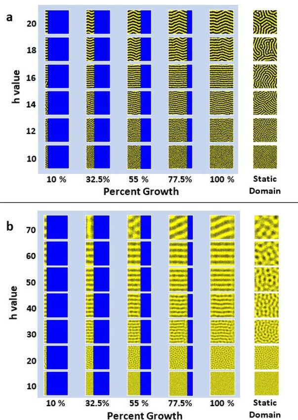
www.nature.com/scientificreports/
Deriving mean field and continuous mean field equations. To investigate the dynamics of the Sur-
vival model, we use both stochastic Monte Carlo simulations and deterministic evolution equations. For the
evolution equations, we consider the ensemble averages of the Boolean variables Xi , Mi , and Si at each lattice
node i, which are given by Xi
, Mi
, and Si
respectively. Using mass-action laws to derive the master equation
for this system, and assuming there is no statistical correlation across space (commonly called the mean field
assumption, where �Ai , Bj � ≃ �Ai ��Bj �), we obtain the following system of ordinary differential equations:
d�Xi � 1
= bX �Si � − dX �Xi � − sM �Xi �(�Mi+1 � + �Mi−1 �) (1)
dt 2
d�Mi � 1 1
= bM �Si � − sX �Mi �(�Xi+1 � + �Xi−1 �) − dMX �Mi � �Xi+h � + �Xi−h �
dt 2 2
(2)
1
− dM �Mi � �Si+h � + �Si−h � + �Mi+h � + �Mi−h �
2
Note that we do not require a separate equation for Si
because the three variables at site i are related by the
balance �Si � = 1 − �Xi � − �Mi �.
We transform Eqs. (1)–(2) into a system of partial differential equations (PDEs) by switching to a continuous
spatial coordinate r = ia, where a is the average diameter of a cell, on which we define the continuous field vari-
ables x = x(r) = �Xi � and m = m(r) = �Mi �, which are assumed to change smoothly over r. Using a second-order
Taylor series expansion in r, we obtain the following continuous mean field PDE system:
∂x a2
= bx (1 − x − m) − dx x − sM mx − sM x∇ 2 m (3)
∂t 2
a2 h2 a 2 h2 a 2
∂m
= bM (1 − x − m) − dM m − (−dM + dMX + sX )xm − sX m + dMX m − dM m ∇ 2 x
∂t 2 2 2
(4)
It is important to remember that the apparent cross-diffusion terms in Eqs. (3)–(4) do not represent true
diffusion, but rather are a result of the continuous approximation of the short-range and long-range discrete
interactions. While Eqs. (1)–(4) describe a one-dimensional lattice (Eqs. (1)–(2)) or one-dimensional coordi-
nate system (Eqs. (3)–(4)), the same derivation can be used to extend the system to higher dimensions. For the
theoretical basis for the lattice approach to modeling and the equations, see the Methods section.
Spatial patterns arising from the Survival model are Turing‑type patterns. We use a variety of
methods to study the Survival model and show how it can generate Turing patterns. In the simulations presented
here, we limit ourselves to an idealized case where we assume that the short-range mutual inhibition rate con-
stants are identical ( sX = sM = s) and that the death of xanthophores is caused only by short-range and long-
range interactions, and not by simple decay (dX = 0). In addition, we assume that the “survival” signal given
to the melanophores by the xanthophores effectively prevents the melanophores from dying (dMX = 0). While
biologically unrealistic, these approximations allow us to qualitatively represent the dynamic behavior of the
odel31, which
system, as well as allow a closer comparison to the previously published results of the Promotion m
were obtained under similar assumptions.
To begin, we perform a linear stability analysis (LSA) on the continuous mean field PDE system (Eqs. (3)–(4))
under the conditions of our simulations (dX = dMX = 0, sX = sM = s ). A detailed description of the LSA is
included in the the Methods section. The system admits two homogeneous steady states:
x1 = 1, m1 = 0 (5)
bX dM (bM − bX )s
x2 = , m2 = . (6)
bX (dM − s) + bM s bX (dM − s) + (bM + dM )s
The LSA shows that when the parameter h is larger than a critical value hT (which is controlled by the values
of the other parameters), the second steady state can undergo a Turing bifurcation, which is generally associ-
ated with spontaneous generation of stationary patterns like those observed in the MC simulations. The Turing
bifurcation arises in response to a perturbation of wavenumber kT , and at the bifurcation point would generate a
pattern with the critical wavelength T = 2π/kT . For more details of these calculations, see the Methods section.
We then compare the results of the LSA to simulations of the one-dimensional mean field equations
(Eqs. (1)–(2)) on a lattice of size n = 50 with periodic boundary conditions, as shown in Fig. 2. The simulations
are extended vertically for ease of viewing and show the normalized concentration of xanthophores at each lat-
tice node ( Xi
). The blue curves in Fig. 2a,b show the bifurcation parameter hT , and the orange curve shows half
the critical wavelength T /2. Based on the LSA, we would expect to see Turing patterns everywhere above the
blue hT curve. However, when we examine the absolutely scaled (between 0 and 1) mean field simulations, we
see that large amplitude patterns only form for part of the parameter space (Fig. 2a). It is only when we examine
the relatively scaled (between the minimum and maximum Xi
values for that simulation) simulations that
Turing patterns can be distinctly seen for all the parameter values in the region past the Turing bifurcation point
(Fig. 2b). So although the LSA correctly predicts the region of the parameter space where patterns emerge, it
cannot account for the fact that some of these patterns have an extremely small amplitude.
Scientific Reports | (2021) 11:9864 | https://doi.org/10.1038/s41598-021-89116-4 4
Vol:.(1234567890)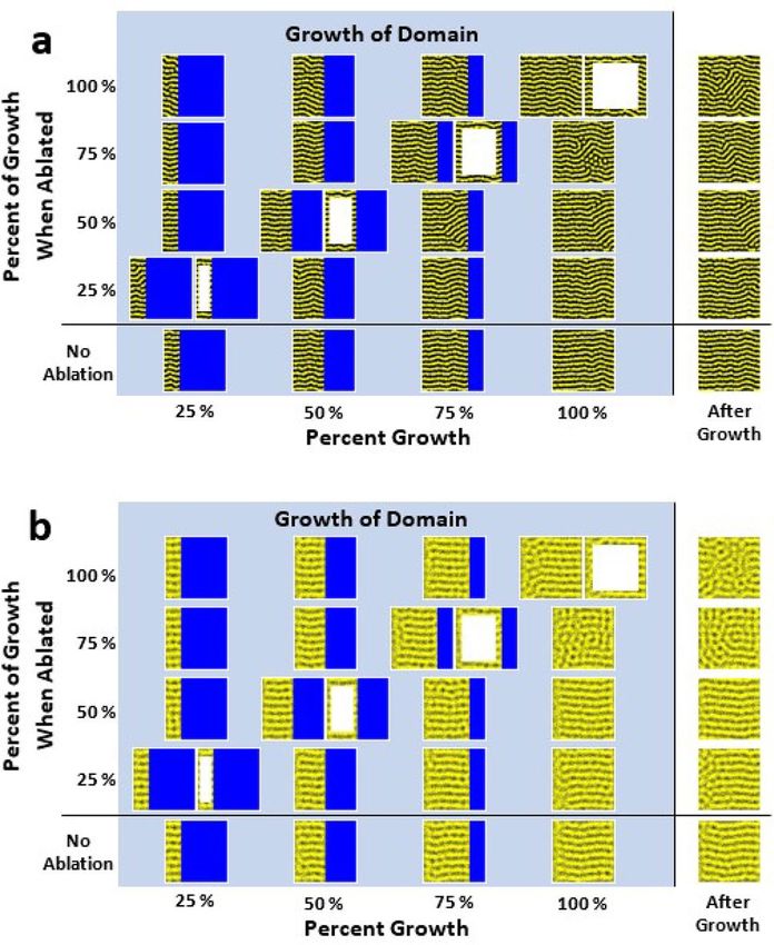
www.nature.com/scientificreports/
Figure 2. Numerical simulations and results of LSA of the Survival model in one dimension. For each
numerical simulation, Eqs. (1) and (2) were simulated on a size n = 50 lattice with periodic boundaries. The
xanthophore concentration ( Xi
) is shown. The results were extended vertically into a square shape for ease
of viewing. The following conditions were held constant in all simulations and when performing the LSA:
bX = s = 1, dX = dMX = 0. (a) and (b) Simulations of the Survival model for various long-range interaction
distances h and melanophore birth rates bM . The death rate of melanophores was held constant at dM = 4. The
blue curve is a plot of the minimum long-range interaction distance hT that allows for Turing patterns, and the
orange curve is one-half of the critical wavelength ( T /2). The simulations in (a) and (b) are identical, but (a) is
absolutely scaled between a normalized concentration of zero and one, while (b) is relatively scaled between the
minimum and maximum values of Xi
for that simulation. (c) Simulations of the Survival model for various bM
and dM parameter combinations. For all simulations, the long-range interaction distance was held constant at
h = 15. The red line approximately indicates the onset of patterning at hT = T /2. (d) Analytical result of LSA
of the continuous mean field Eqs. (3)–(4). The cyan surface is a plot of the bifurcation value hT , the critical long-
range interaction distance. The orange surface is a plot of half the critical wavelength, T /2. The red curve shows
the intersection of the two surfaces, where hT = T /2.
We also explore the relationship between multiple Survival model “reaction” parameters. In Fig. 2c, we show
simulations of the mean field equations (Eqs. (1)–(2)) at a constant long-range interaction distance h = 15 as
we vary the birth and death rates of melanophores (bM and dM respectively). We observe that large-amplitude
patterns form only when dM > bM s (we have marked the dM = bM s line in red in Fig. 2c). Below this (when
bM s > dM ), the patterns have a much smaller amplitude and are not visible in the absolutely scaled images.
Interestingly, this line, beyond which patterns can form, also corresponds to the curve hT = T /2 when the
surfaces of hT (cyan) and T /2 are plotted for these bM and dM ranges (Fig. 2d). The correspondence between the
Scientific Reports | (2021) 11:9864 | https://doi.org/10.1038/s41598-021-89116-4 5
Vol.:(0123456789)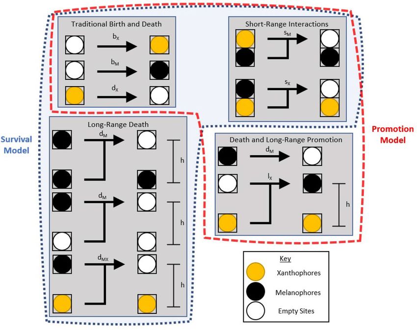
www.nature.com/scientificreports/
sharp transition line from small-amplitude to large-amplitude patterns and the curve where hT = T /2 persists
when parameters bX and s are varied (in Fig. 2, they were fixed at 1). Currently, we are investigating the origin
of this sharp increase in pattern amplitude - potentially as a spatial analog in our multiple length scale system
of the temporal canard explosion found in some temporally oscillating systems with multiple time s cales40–42.
The Survival model produces Turing patterns with disperse melanophore stripes. The one-
dimensional mean field simulations and the LSA demonstrate that the patterns resulting from the Survival
model are the result of a Turing-type instability. To show the patterns on a two-dimensional domain, we first use
a stochastic Monte Carlo method on a static lattice (Fig. 3a). A full description of our simulation algorithm is
located in the Methods section, and the code used is available in the Code Availability Section. Figure 3a shows
that the relationship between the birth rate of melanophores bM and their long-range death rate dM determines
whether a pattern is robust enough to be distinguished from the stochastic noise. When we compare these results
to deterministic ODE simulations of the two-dimensional mean field equations, we see that the spotted patterns
are the only ones that form with a large enough amplitude to be seen with absolute scaling (Fig. 3b) instead of
relative scaling (Fig. 3c). However, Turing patterns still exist in the same region of parameter space predicted
by the LSA of Eqs. (3)–(4), which is the area below and to the right of the hT asymptotes (Fig. 2d, cyan curve)
marked by the red lines in Fig. 3. When patterns only have small amplitudes, they appear to be overwhelmed by
noise in the stochastic simulations, as evidenced in the lower left region of Fig. 3a.
Simulations with different h values also show that the pattern wavelength - the distance between two stripes of
the same color - is roughly given by 2h, as seen in Fig. 4. Similar qualitative relationships between stripe distance
(pattern wavelength) and the long-range interaction distance found in simulations of the Survival model are also
seen in the Promotion m odel31 and agent-based m odels29,30. However, the stochastic simulations of the Survival
model show that the areas with melanophores (stripes and spots) are significantly less melanophore-dense than
in the Promotion model, with large numbers of xanthophores located in the melanophore stripes (Figs. 3a, 4).
In simulations of the Promotion m odel31, melanophore and xanthophore stripes are almost entirely comprised
of one chromatophore, with very little intermixing. One possible explanation of this difference is that the sur-
vival feedback constitutes a somewhat weaker form of positive feedback than the promotion of new cells. If so,
the Survival model may be more strongly affected by the inherent stochastic noise than the Promotion model.
We note that that the more “blurred” distribution of cells in the Survival model is closer to that in the actual
zebrafish, as loosely-packed xanthophores are found in the stripes of melanophores and more densely-packed
xanthophores are isolated in the i nterstripes15,19,22,28.
Domain growth orients Turing patterns. We examined the impact of domain growth on Turing pat-
tern development in both the Promotion and Survival models (Fig. 5). For this study, we used stochastic Monte
Carlo simulations implemented on a lattice, as this yielded morphological behavior similar to deterministic
ODE simulations of the mean field equations (Eqs. (1)–(2)) at a fraction of the computing cost. Domain growth
was implemented by adding a column of empty lattice sites to the existing lattice after a set number of iterations
of the simulation algorithm. See the Methods section for a complete description of the algorithm and the Code
Availability section for the code developed for the Survival model simulations. Animations of the the growing
simulations for h = 10 and h = 16 in Fig. 5a (Promotion) and for h = 20 and h = 50 in Fig. 5b (Survival) are
contained in the Supplementary Information. Note that for all simulations, we used rate parameters that forced
stripe patterns, as it is difficult to distinguish how growth affects spotted patterns, as previously observed in
reaction-diffusion systems37.
Figure 5 shows that domain growth greatly influences the orientation of the Turing patterns in both the
Promotion and Survival models (Fig. 5a,b, respectively). In the Promotion model, for h ≥ 12, the Turing pat-
terns orient themselves perpendicular to the growing boundary, as shown in Fig. 5a. For larger values of h, the
stripes become a bit wavy, but overall are still relatively perpendicular to the growing boundary. This is especially
evident when compared to the lack of orientation of the static domain simulations under the same conditions
(Fig. 5a, right side).
Simulations of the Survival model on a growing domain show results qualitatively similar to the Promotion
model. Domain growth still orients the Turing patterns perpendicular to the growing boundary above a specific
value of h (Fig. 5). However, for the Survival model, the stripes orient themselves in this manner only for h ≥ 30, a
much higher value than in the Promotion model. This is evident in the simulations shown in Fig. 5b, as the result-
ing Turing patterns for h = 10 and 20 show no orientation and look similar to their static domain counterparts.
The pattern orientation behavior for various h values occurs regardless of the domain size or shape, as long as
the domain is large enough to allow for multiple wavelengths ( ≈ 2h). If the domain is unable to contain more
than a few wavelengths and its length is not near an integer multiple of a stable wavelength, the stripes may orient
obliquely relative to the growing boundary, as seen for the pattern with long-range interaction distance h = 70
( ≈ 140) for the Survival model in Fig. 5b. If the growth is not one-dimensional (for example, a trapezoid that
grows from one side as a model of fin growth, as shown in Supplementary Figure S1) the patterns still orient
themselves horizontally with the growing boundary. The stripes added during growth are not affected by any
previously formed patterns, as shown in Supplementary Fig. S2. These results show that domain growth signifi-
cantly affects Turing pattern development and orientation, even in the absence of a pre-pattern. This suggests
that growth may play a significant factor in zebrafish skin pattern orientation, especially in the tail and anal fins,
which lack iridophores and the horizontal m yoseptum18,23,38,43.
Growth can reorient stripes in ablated cells. Laser ablation of zebrafish chromatophores has often
atterns14,15,21,22,28,29. To simulate this behavior,
been used to study the cellular mechanisms that form their skin p
Scientific Reports | (2021) 11:9864 | https://doi.org/10.1038/s41598-021-89116-4 6
Vol:.(1234567890)www.nature.com/scientificreports/
Figure 3. Numerical simulations of the Survival model on a two-dimensional 50 × 50 lattice with periodic
boundary conditions. In all figures, bM and dM were varied from 0 to 10 (top to bottom and left to right,
respectively). The following parameters were held constant: h = 15, bX = s = 1, dX = dMX = 0. The red lines
indicate the area where Turing patterns are predicted by the LSA. (a) Stochastic Monte Carlo simulations.
Each simulation began on a uniform initial condition corresponding to an empty lattice. Yellow, black, and
white lattice sites represent xanthophores, melanophores, and empty sites respectively. (b) and (c) Numerical
integration of the two dimensional mean field equations describing the Survival model. Each simulation
started from random initial conditions and ran for 1000 time steps. (b) shows the normalized concentration of
xanthophores ( Xi,j
) scaled absolutely between zero and one. (c) shows the same simulations scaled relative to
each simulation’s maximum and minimum.
we “ablated” the central lattice sites of growing pattern simulations at different percentages of growth (Fig. 6).
To ablate the pattern, we replaced the middle 75% of the rows and columns in the simulation with empty cells
(white) in the stochastic Monte Carlo simulations. The simulations then continued to grow until they reached
their final size, and then the simulation was continued on a static domain to see if the resulting patterns were spa-
tially stable (Fig. 6, “After Growth” column). A simulation with no ablation is shown in the bottom row of Fig. 6a
and b for comparison. Animations of the the simulations ablated at 50% and 100% for both the Promotion model
(Fig. 6a) and the Survival model (Fig. 6b) are included in the Supplementary Information.
Scientific Reports | (2021) 11:9864 | https://doi.org/10.1038/s41598-021-89116-4 7
Vol.:(0123456789)www.nature.com/scientificreports/
Figure 4. Stationary Turing patterns with varying h values in Monte Carlo simulations of the Survival model.
Each simulation was performed on a 400 × 400 static lattice with periodic boundary conditions. The following
parameters were held constant: bM = 7, dM = 9, bX = s = 1, dX = dMX = 0. For each pattern shown, the first
digit of the h value is given by the row label and the second digit is given by the column label. For example, the
Turing pattern in the fifth row and third column has h = 54.
Simulations of the Promotion and Survival models (Fig. 6a and b, respectively) with ablation show very
similar behavior. If ablation occurs once the growth is complete (top row in Fig. 6a,b), the patterns will reform
in a random orientation where the ablation occurs (rightmost column in Fig. 6a,b). However, if ablation occurs
early during growth (for example, 25% or 50% of growth completed), the pattern recovers to an orientation
perpendicular to the growing boundary, as if the pattern had not been ablated at all (shown for comparison in
bottom rows of Fig. 6a,b). These behaviors are qualitatively very similar to what occurs for both fully-developed
adult14,15 and developing44 zebrafish when their patterns are ablated.
Discussion
We have proposed the “Survival model,” a simplified reaction scheme that can generate Turing patterns on a
lattice in the absence of cellular movement. Instead, Gierer and Meinhardt’s SRALRI conditions are met via
short-range competition between the two chromatophores (leading to self-activation) and having xanthophores
enhance the survival of melanophores at longer distances (Fig. 1). This model is inspired by multiple experimen-
tal studies on zebrafish pattern formation19,21,22,45. In particular, the “Survival” feedback corresponds to a Delta/
Notch signalling pathway found in adult zebrafish: melanophores extend a projection towards xanthophores,
which then carries a signal essential to melanophore survival15,22,23. These projections reach a maximum size of
half the stripe width. The Survival model is particularly applicable to the patterns on the tail and anal fins of the
zebrafish. Unlike the body, where iridophores are necessary for pattern formation18,43, the patterns formed on the
tail and anal fins are produced without other chromatophores present44,45. In addition, melanophore movement
is heavily restricted on the zebrafish fins, justifying the approximation of immobile cells44,46.
The Survival model in this paper incorporates many of the same interactions as the previously-published
Promotion model31, as shown in Fig. 1. The only significant difference is the nature of the long-range interaction.
When comparing the Monte Carlo simulations of the Survival lattice on a static domain (Figs. 3a, 4) to those
of the Promotion model in R eference31, one can see that the melanophore stripes/spots are much less dense in
the Survival model. This may indicate that a “Survival” interaction constitutes a weaker form of feedback than
a “Promotion” interaction. Yet, even this weaker long-range interaction is sufficient to induce Turing patterns
over a wide variety of conditions (Figs. 2, 3). It is also worth noting that the more diffuse melanophore stripes
resemble the melanophore stripes found on actual zebrafish15 more closely than the more homogeneous stripes
seen in the Promotion model simulations.
In addition to studying a new type of long-range interaction in the Survival model, we have also investigated
the impact of domain growth, a process that has not previously been considered in either the Survival or the
Promotion model. Our stochastic simulations of the two models on growing domains indicate that growth has
a major impact on pattern development and orientation. The simulations in Figs. 5 and 6 show that growth can
orient patterns perpendicular to the growing boundary. Even when a defect in the pattern occurs, such as abla-
tion, if the system is still growing, the pattern will spontaneously reorient itself. These are particularly interesting
results as the lattice nodes themselves are not actually moving - only new nodes are added. Yet, similar behav-
ior is shown in other, more traditional reaction-diffusion systems on growing domains in experimental36,37,47,
Scientific Reports | (2021) 11:9864 | https://doi.org/10.1038/s41598-021-89116-4 8
Vol:.(1234567890)www.nature.com/scientificreports/
Figure 5. Turing pattern development during domain growth. For each h value, two simulations are
presented: one on a growing domain (light blue backing) and one on a static domain (right column).
For each simulation on a growing domain, images are shown of the developing pattern at 10%, 32.5%,
55%, 77.5%, and 100% of growth. The royal blue areas are the remaining area each simulation will grow
into. All simulations are performed with periodic boundary conditions for the same simulation length.
(a) Stochastic Monte Carlo simulations of the Promotion model on a growing domain. Each simulation
begins as a 300 × 1 lattice, and grows to a final size of 300 × 300. Each simulation is performed with
bX = 1, s = 1, lX = 2.5, bM = dX = dM = 0. (b) Stochastic Monte Carlo simulations of the Survival model
on a growing domain. Each simulation begins as a 400 × 1 lattice, and grows to a final size of 400 × 400. Each
simulation is performed with bX = 1, s = 1, bM = 7, dM = 9, dX = dMX = 0.
agent-based numerical29,30, and analytical9,32,33,35 studies. These results may not demonstrate unequivocally that
domain growth alone is responsible for the parallel stripe orientation on zebrafish tail and anal fins, but they
do indicate that domain growth may play a significant role in ensuring that zebrafish patterns form along the
growth axis in a reproducible m anner21,22,30,48.
While the Survival and Promotion models behave qualitatively similarly on a growing domain (Fig. 5),
simulations of the Survival model require a much large h value (the long-range interaction distance) to orient
perpendicular to the growing boundary. In most zebrafish, the stripes are approximately 10-20 cells wide. Yet,
in the Survival model with growth, the perpendicular orientation only occurs with a stripe width of at least 30
cells (h ≥ 30) for the reaction parameters used here. This suggests that during zebrafish growth, other types of
cellular interactions are likely to be involved in the initial pattern formation. One possible such interaction could
be caused by the airinemes described in Eom et al.21. Airinemes are protrusions extending from xanthophores
located inside melanophore stripes to nearby melanophores. They cause melanophores to consolidate into stripes
during earlier stages of development, but then retract as zebrafish reach m aturity21.
Our studies of the Survival model, its behavior on a growing domain and during ablation have yielded several
interesting results. We have shown that zebrafish pattern formation, particularly on the fins, may arise from a
Turing bifurcation with a new form of the long-range interaction - which was inspired by experimental studies22.
The patterns that result from simulations of this model are consistent with the “Differential Growth” picture
previously proposed by Bullara and De D ecker31 in that Turing-type patterns can arise without morphogen move-
ment, even when the Survival feedback is a weaker form of feedback than the Promotion feedback. In addition,
we showed that domain growth can have a significant impact on the pattern orientation for both the Promotion
and Survival models. The growing domain can orient the resulting patterns (albeit at different long-range interac-
tion distances depending on the model), just as it can for traditional reaction-diffusion systems with morphogen
Scientific Reports | (2021) 11:9864 | https://doi.org/10.1038/s41598-021-89116-4 9
Vol.:(0123456789)www.nature.com/scientificreports/
Figure 6. Ablation of Turing patterns at different percentages of growth. Simulations with the same conditions
(one per row) were ablated at 25%, 50%, 75%, 100% of their total growth. The middle 75% of the domain was
ablated (right side of each dual image—left side is simulation directly before ablation). Once the growth was
complete, the simulations continued to run for ≈ 17% of the time of growth to observe the stability of the
final pattern (far right of each simulation). (a) Growth simulations of the Promotion model with ablation. The
domain grows from a 300 × 1 cell lattice to a 300 × 300 cell lattice. The conditions of each simulation (rows)
are: h = 14, bX = 1, s = 1, lX = 2.5, bM = dM = dX = 0. (b) Growth simulations of the Survival model
with ablation. The domain grows from a 400 × 1 cell lattice to a 400 × 400 cell lattice. The conditions of each
simulation (rows) are: h = 30, bX = 1, s = 1, bM = 7, dM = 9, dX = dMX = 0.
diffusion35–37,49,50. In the future, it should be possible to update our model to account for additional intercellular
interactions in order to provide a more complete understanding of the morphogenesis occurring on the skin
of the zebrafish. It may also be of interest to examine pattern-forming behavior in other natural systems, such
as the positional information-guiding cytonemes in drosophila51 or the reaction-diffusion-advection models of
synaptogenesis in C. elegans52, using the modeling techniques employed in this work.
Methods
Theoretical approach for the lattice‑based model. To model the zebrafish skin, we use a lattice of
size N where each node i = 1, 2, ..., N can be occupied by either a a xanthophore ( Xi ) or a melanophore ( Mi )
or remain empty (Si ). We define the “state” of the system by specifying the occupancy of each node (X, M, or
S). Thus, there are 3N possible states of the system. Transitions between states are determined in a probabilistic
manner based on the rate constants of the various interactions.
We use two approaches to simulate the system and show that patterns can develop. The first method is stochas-
tic simulation using a Monte Carlo algorithm which is described in detail in a later subsection of the Methods.
Each simulation is one realization of the system evolving in time via a Markovian process - where at most one
event can occur per unit time. Examples of non-growing simulations of this type are shown in Figs. 3a and 4.
The second method of simulation is deterministic mean-field simulation, whose results are shown in Figs. 2 and
3b,c in the main text. Instead of simulating one instance of the system’s time evolution, the mean field equations
(Eqs. (1)–(2) in the main text) describe the average behavior of an ensemble of realizations of the system. A full
description of the equations and methods used for the deterministic mean-field simulations is given later in the
Methods. In addition, a set of continuous mean-field equations (Eqs. (3)–(4) in the main text) can be derived
from the mean field equations using a second-order Taylor series expansion. These are used to show that a
Turing-type mechanism guides the pattern formation in the Survival model.
Turing analysis. To determine whether the continuous mean field equation system is capable of undergo-
ing a Turing-type bifurcation, we perform a linear stability analysis on a simplified version of Eqs. (3) and (4).
Specifically, we are looking for a homogeneous steady state that is stable without the spatially dependent terms,
Scientific Reports | (2021) 11:9864 | https://doi.org/10.1038/s41598-021-89116-4 10
Vol:.(1234567890)www.nature.com/scientificreports/
but becomes unstable when the cross diffusion-like terms are added. We define a general reaction-diffusion
system as
∂c
= R (c) + D ∇ 2 c (7)
∂t
where c is a vector of morphogen concentrations, R (c) are the reaction terms, and D is a matrix of the diffusion
coefficients. We calculate the steady states (in the absence of diffusion) by solving
R (c0 ) = 0
and denote the Jacobian J of the reaction vector function R at the point c0 as
dR (c)
J =
dc c=c0
A Turing instability occurs when the system is in a stable steady state at c0 , and then is destabilized by a
spatial perturbation of nonzero wavenumber k. The steady state c0 is stable with respect to spatially homogene-
ous perturbations when the real parts of the eigenvalues of the Jacobian matrix J are all negative, which in a
two-variable systems occurs when
Tr(J ) < 0 and Det(J ) > 0 (8)
To examine the spatial instability at wavenumber k, we calculate the linearized matrix of the system (Eq. 7),
L, in the form
L = J − k2 D (9)
If L has a positive eigenvalue (indicating an instability) for a finite, positive wavenumber k, then a Turing
bifurcation has occurred, which produces spatially periodic patterns which are stationary in time. To show this,
we calculate the characteristic equation of the eigenvalue ω , which in a two-variable system takes the form:
ω2 − Tr(L )ω + Det(L ) = 0 (10)
For the system to be unstable and stationary in time, the eigenvalue ω must be greater than zero and have no
imaginary component (ω > 0 and Im(ω) = 0). For the system to be periodic in space, the wavenumber k = 0.
Thus, if we can show that the eigenvalue ω is positive for a positive finite value of k, then a Turing instability
exists for the system.
We can also analytically solve for the Turing bifurcation point; that is, the value at which a perturbation with
critical wavenumber kT becomes unstable. To solve for the bifurcation point, we solve the systems of equations:
∂Det(L )
Det(L ) = 0 and =0 (11)
∂k2
for the critical wavenumber kT and the critical value of a bifurcation parameter (for the Survival model, we will
solve for the critical long-range interaction distance, hT ). In the following subsections, we show that this analysis
holds for a simplified version of the Survival model.
Linear stability analysis of nonuniform steady state. The continuous mean field equations (Eqs. (3)–(4)) are sim-
plified using the assumptions given in the main text. In addition, we assume a = 1, which establishes the space
scale. The resulting simplified PDE system is:
∂x 1
= bX (1 − x − m) − smx − sx∇ 2 m (12)
∂t 2
h2
∂m 1
= bM (1 − x − m) − smx − dM m(1 − x) − sm − dM m ∇ 2 x (13)
∂t 2 2
The steady states of the system (Eqs. (12) and (13)) in the absence of the cross-diffusion terms are given by
Eqs. (5) and (6) in the main text. No Turing bifurcation can occur at the homogeneous steady state (Eq. (5)),
and thus it will not be analyzed further.
To determine the stability of the second steady state (Eq. (6)), we first calculate the Jacobian matrix of the
reaction functions to determine how the functions react to small perturbations. The Jacobian is:
−bX − sm − bX − sx
J =
−bM + dM m − sm − bM − dM + dM x − sx (14)
The Jacobian yields a trace of
Tr(J ) = −bM − bX − dM (1 − x) − s(m + x) (15)
Scientific Reports | (2021) 11:9864 | https://doi.org/10.1038/s41598-021-89116-4 11
Vol.:(0123456789)www.nature.com/scientificreports/
Since by definition x ≤ 1 and all rate constants, x, and m are greater than zero, every term in the trace is
negative. When the determinant of the Jacobian is calculated ( Det(J )) and the steady state values of x = x2 and
m = m2 are substituted, the resulting equation is:
Det(J ) = (bM − bX )s (16)
This meets the stability requirements shown in Eq. (8) when bM > bX . Thus, in the absence of the diffusion-
like terms, the steady state (x2 , m2 ) is stable per the conditions in Eq. (8).
Notice that if we substitute the values of x and m for the first steady states (5) into the condition for the trace
(15) and the determinant (16) of the Jacobian we obtain
Tr(J ) = −bM − bX − s < 0 and Det(J ) = −(bM − bX )s (17)
which predicts that the uniform steady state becomes a saddle point (and therefore unstable) as bM > bX . In
other words, for bM = bX we have a transcritical bifurcation through which the two steady states of the systems
exchange stability.
Turing bifurcation. To determine whether steady state (x2 , m2 ) is stable with regard to spatial perturbations, we
first construct the “diffusion” matrix D as
0 − 2s x
D = h2 s
2 dM m − 2 m 0
From here, we can construct the linearized matrix L as per Eq. (9):
− bX − sx + k2 2s x
−bX − sm
L = (18)
2
−bM + dM m − sm − k2 h2 dM m − 2s m − bM − dM + dM x − sx
We can then solve for the bifurcation parameter hT and critical wavenumber kT using the conditions in
Eq. (11). A plot of twice the critical long-range interaction distance (hT ) is shown in cyan in Fig. 2. The critical
wavenumber can also be converted into the critical wavelength T using the relationship
2π
T =
kT
The blue curve plotted in Fig. 2 is T /2. Thus, for every value of h > hT the second steady state is unstable to
linear spatial perturbations. It will form spatial patterns; however, the patterns can sometimes have very small
amplitudes and thus are only visible under certain parameters (see Figs. 2a,b and 3b,c).
Deterministic mean field simulations. We simulate the deterministic behaviors of the system for a static
domain by numerically solving Eqs. (1) and (2) on a n = 50 one-dimensional lattice in Fig. 2. We perform the
numerical simulations in MATLAB using the solver ode23s. The state of each node is given by the relative occu-
pancy (ranging from 0 to 1) of each chromatophore. Normalized concentrations of xanthophores are shown in
Fig. 2a,c. Simulations where the normalized concentrations were scaled between their maximum and minimum
values are shown in 2b. The same methods were used to simulate the corresponding two-dimensional mean field
equations on a 50 x 50 lattice in Fig. 3b,c.
Stochastic Monte Carlo simulations. The actual simulations (described below) were performed using a
custom-developed C++ package. Then, the .csv files that were exported during the simulations were converted
to image files using the Python package zebrafish_plot. This package also produces the animations of grow-
ing simulations, examples of which are found in the Supplementary Information. Descriptions of the C++ and
Python package algorithms are below, and a link to the code is given in Code Availability section.
Base algorithm with survival model. The simulation algorithm for the Survival model on a static domain is
similar to the algorithm used in Bullara et al. for the Promotion model31. A brief description of the algorithm on
a static (non-growing) domain is:
1. A rectangular lattice with periodic boundary conditions is generated with a predefined number of rows and
columns. Each lattice node has four first neighbors and can be occupied by either an empty space (S, 0 in the
exported .csv files), a xanthophore (X, 1 in the exported .csv files), or a melanophore (M, 2 in the exported
.csv files). The lattice can be initialized as empty (all nodes are S), a random distribution of chromatophores
and empty sites (random assortment of X, M, and S), or with all xanthophores or melanophores. In all of the
simulations shown in this article, the lattice starts as empty.
2. Probabilities for each reaction shown in Fig. 1 for the Survival model are calculated as the rate constant
divided by the sum of all of the rate constants.
3. A predefined number of iterations of the Monte Carlo algorithm is chosen to ensure that a stable pattern
will form. For the static simulations in Figs. 3a and 4 in the main text, the number of iterations is set to 109.
For each iteration, one lattice node (say position k) is selected at random, and one of the reaction process
shown in Fig. 1 in the main text is selected at random with the appropriate probability. If the process selected
Scientific Reports | (2021) 11:9864 | https://doi.org/10.1038/s41598-021-89116-4 12
Vol:.(1234567890)www.nature.com/scientificreports/
involves another lattice node (short-range or long-range interactions), a nearest neighbor (short-range inter-
action) or node a distance h away (long-range interaction) is chosen at random to determine whether the
process condition is met. If the conditions for the process are met, the lattice is updated.
4. Comma-separated values files (.csv) of the two-dimensional lattice state are exported after a specific number
of iterations, as defined in the code.
5. After all iterations are complete, the final lattice is exported along with a .csv file containing all of the relevant
parameters used in the simulation.
Implementing domain growth and ablation. The above algorithm was modified to include domain growth.
Instead of defining the size of the domain and the number of iterations of the Monte Carlo algorithm steps, we
choose the initial size of the domain, the number of iterations before growth, and the number of growth events.
When the simulation reaches the desired number of iterations, new lattice nodes are added to one side, and
the nearest neighbors are updated with the new nodes. The added nodes can either be identical to an adjacent
column or all empty. For all of the growth shown in Figs. 5 and 6 in the main text, an empty column was added
at each growth event, which occurred every 107 iterations. There are functions in the Code Availability section
that allow for trapezoidal growth, where both rows and columns are added. In addition, the user can specify the
number of iterations before growth starts or after it is complete.
In a similar manner, ablation is performed by setting a code variable to specify when the user wants to ablate
the system. When the simulation reaches the point of ablation, it converts a percentage of the middle rows and
middle columns to empty sites (S). For the simulations shown in Fig. 6, the middle 75% of rows and the middle
75% of columns were ablated.
Converting output to image files and animations. Once a simulation is complete, the exported .csv files were
converted to the individual .png files shown in Figs. 3a, 4, 5, and 6 as well as Supplemental Figs. S1 and S2 in
Python. For each imported .csv file, an array of the largest array size was created and was colored according to
the numeric value in the .csv file. For xanthophores (value of 1 in the .csv file), the image array was colored yel-
low, and for melanophores (value of 2 in the .csv file), the image array was colored black. Empty sites were left as
white, and if the image array was larger than the current .csv file array (because growth had not been completed
yet) the remainder of the image array was colored blue. Each of the resulting image arrays was exported to a
subfolder within the folder containing the original .csv files. Then, the image files were knitted together into an
animation, which was saved into the same subfolder.
Code Availability
The code developed for this study is available in the EpsteinLab Github. The Survival-MC and Zebrafish-Plot
repositories specifically are used. Link: https://github.com/EpsteinLab.
Received: 29 January 2021; Accepted: 14 April 2021
References
1. Turing, A. M. The chemical basis of morphogenesis. Philos. Trans. R. Soc. B Biol. Sci. 237, 37–72 (1952) (ISSN: 0962-8436).
2. Green, J. B. & Sharpe, J. Positional information and reaction–diffusion: two big ideas in developmental biology combine. Develop-
ment 142, 1203–1211 (2015).
3. Gierer, A. & Meinhardt, H. A theory of biological pattern formation. Kybernetik 12, 30–39 (1972) (ISSN: 0340-1200).
4. Meinhardt, H. & Gierer, A. Pattern formation by local self-activation and lateral inhibition. BioEssays 22, 753–760 (2000) (ISSN:
02659247).
5. Meinhardt, H. Turing’s theory of morphogenesis of 1952 and the subsequent discovery of the crucial role of local self enhancement
and long-range inhibition. Interface Focus 2, 407–416 (2012) (ISSN: 20428901).
6. Castets, V., Dulos, E., Boissonade, J. & De Kepper, P. Experimental evidence of a sustained standing Turing-type nonequilibrium
chemical pattern. Phys. Rev. Lett. 64, 2953–2956 (1990).
7. Ball, P. Forging patterns and making waves from biology to geology: a commentary on Turing (1952) ‘The chemical basis of
morphogenesis’. Philos. Trans. R. Soc. B Biol. Sci. 370, 20140218 (2015) (ISSN: 0962-8436).
8. Ermentrout, B. & Lewis, M. Pattern formation in systems with one spatially distributed species. Tech. Rep. 3, 533–549 (1997).
9. Klika, V., Baker, R. E., Headon, D. & Gaffney, E. A. The influence of receptor-mediated interactions on reaction–diffusion mecha-
nisms of cellular self-organisation. Bull. Math. Biol. 74, 935–957 (2012) (ISSN: 0092-8240).
10. Lengyel, I. & Epstein, I. R. Modeling of Turing structures in the chlorite-iodide-malonic acid-starch reaction system. Science 251,
650–652 (1991).
11. Kondo, S. & Asai, R. A reaction-diffusion wave on the skin of the marine angelfish Pomacanthus. Nature 376, 765–768 (1995)
(ISSN: 0028-0836).
12. Lefèvre, J. & Mangin, J. F. A reaction-diffusion model of human brain development. PLoS Comput. Biol.https://doi.org/10.1371/
journal.pcbi.1000749 (ISSN: 1553734X).
13. Liu, R. T., Liaw, S. S. & Maini, P. K. Two-stage Turing model for generating pigment patterns on the leopard and the jaguar. Phys.
Rev. E 74, 011914 (2006) (ISSN: 1539-3755).
14. Yamaguchi, M., Yoshimoto, E. & Kondo, S. Pattern regulation in the stripe of zebrafish suggests an underlying dynamic and
autonomous mechanism. Proc. Natl. Acad. Sci. U. S. A. 104, 4790–4793 (2007) (ISSN: 00278424).
15. Nakamasu, A., Takahashi, G., Kanbe, A. & Kondo, S. Interactions between zebrafish pigment cells responsible for the generation
of Turing patterns. Proc. Natl. Acad. Sci. U. S. A. 106, 8429–34 (2009) (ISSN: 1091-6490).
16. Gates, M. A. et al. A genetic linkage map for zebrafish: comparative analysis and localization of genes and expressed sequences.
Genome Res. 9, 334–347 (1999) (ISSN: 10889051).
17. Kondo, S. & Miura, T. Reaction-diffusion model as a framework for understanding biological pattern formation. Science (New
York, N.Y.) 329, 1616–20 (2010) (ISSN: 1095-9203).
Scientific Reports | (2021) 11:9864 | https://doi.org/10.1038/s41598-021-89116-4 13
Vol.:(0123456789)www.nature.com/scientificreports/
18. Frohnhöfer, H. G., Krauss, J., Maischein, H. M. & Nüsslein-Volhard, C. Iridophores and their interactions with other chromato-
phores are required for stripe formation in zebrafish. Development (Cambridge) 140, 2997–3007 (2013) (ISSN: 09501991).
19. Nüsslein-Volhard, C. & Singh, A. P. How fish color their skin: a paradigm for development and evolution of adult patterns. BioEs-
says 39, 1600231 (2017) (ISSN: 02659247).
20. Mahalwar, P., Walderich, B., Singh, A. P. & Nüsslein-Volhard, C. Local reorganization of xanthophores fine-tunes and colors the
striped pattern of zebrafish. Science (New York, N.Y.) 345, 1362–4 (2014) (ISSN: 1095-9203).
21. Eom, D. S., Bain, E. J., Patterson, L. B., Grout, M. E. & Parichy, D. M. Long-distance communication by specialized cellular projec-
tions during pigment pattern development and evolution. eLife 4, 12401 (2015).
22. Hamada, H. et al. Involvement of Delta/Notch signaling in zebrafish adult pigment stripe patterning. Development (Cambridge)
141, 318–324 (2014) (ISSN: 09501991).
23. Parichy, D. M. & Turner, J. M. Zebrafish puma mutant decouples pigment pattern and somatic metamorphosis. Dev. Biol. 256,
242–257 (2003) (ISSN: 00121606).
24. Scholes, N. S., Schnoerr, D., Isalan, M. & Stumpf, M. P. A comprehensive network atlas reveals that Turing patterns are common
but not robust. Cell Syst. 9, 243–257 (2019) (ISSN: 24054712).
25. Singh, A. P., Frohnhöfer, H.-G., Irion, U. & Nüsslein-Volhard, C. Response to Comment on “Local reorganization of xanthophores
fine-tunes and colors the striped pattern of zebrafish’’. Science 348, 297 (2015).
26. Woolley, T. E., Maini, P. K. & Gaffney, E. A. Is pigment cell pattern formation in zebrafish a game of cops and robbers?. Pigment
Celll Melanoma Res. 27, 686–687 (2014).
27. Watanabe, M. & Kondo, S. Comment on “Local reorganization of xanthophores fine-tunes and colors the striped pattern of
zebrafish” Apr. 2015. https://doi.org/10.1126/science.1261947.http://science.sciencemag.org/.
28. Kondo, S. An updated kernel-based Turing model for studying the mechanisms of biological pattern formation. J. Theor. Biol. 414,
120–127 (2017).
29. Volkening, A. & Sandstede, B. Modelling stripe formation in zebrafish: an agent-based approach. J. R. Soc. Interface 12, 20150812
(2015).
30. Volkening, A. et al. Modeling stripe formation on growing zebrafish tailfins. Bull. Math. Biol. 82, 56 (2020) (ISSN: 15229602).
31. Bullara, D. & De Decker, Y. Pigment cell movement is not required for generation of Turing patterns in zebrafish skin. Nat. Com-
mun. 6, 6971 (2015) (ISSN: 2041-1723).
32. Klika, V. & Gaffney, E. A. History dependence and the continuum approximation breakdown: the impact of domain growth on
Turing’s instability. Proc. R. Soc. A Math. Phys. Eng. Sci. 473, 20160744 (2017) (ISSN: 1364-5021).
33. Madzvamuse, A., Gaffney, E. A. & Maini, P. K. Stability analysis of non-autonomous reaction–diffusion systems: the effects of
growing domains. J. Math. Biol. 61, 133–164 (2010) (ISSN: 0303-6812).
34. Hetzer, G., Madzvamuse, A. & Shen, W. Characterization of Turing diffusion-driven instability on evolving domains. Discrete
Cont. Dyn. Syst. 32, 3975–4000 (2012) (ISSN: 1078-0947).
35. Van Gorder, R. A., Klika, V. & Krause, A. L. Turing conditions for pattern forming systems on evolving manifolds. J. Math. Biol.
82, 4 (2021) (ISSN: 0303-6812).
36. Míguez, D. G., Dolnik, M., Muñuzuri, A. P. & Kramer, L. Effect of axial growth on Turing pattern formation. Phys. Rev. Lett. 96,
048304 (2006) (ISSN: 0031-9007).
37. Konow, C., Somberg, N. H., Chavez, J., Epstein, I. R. & Dolnik, M. Turing patterns on radially growing domains: experiments and
simulations. Phys. Chem. Chem. Phys. 21, 6718–6724 (2019) (ISSN: 1463-9076).
38. Hiscock, T. W. & Megason, S. G. Orientation of Turing-like patterns by morphogen gradients and tissue anisotropies. Cell Syst. 1,
408–416 (2015) (ISSN: 2405-4712).
39. Inaba, M., Yamanaka, H. & Kondo, S. Pigment pattern formation by contact-dependent depolarization. Science 335, 677 (2012)
(ISSN: 10959203).
40. Krupa, M. & Szmolyan, P. Relaxation oscillation and canard explosion. J. Differ. Equ. 174, 312–368 (2001) (ISSN: 00220396).
41. Krupa, M. & Szmolyan, P. Extending geometric singular perturbation theory to nonhyperbolic points-fold and canard points in
two dimensions. SIAM J. Math. Anal. 33, 286–314 (2001) (ISSN: 00361410).
42. Rotstein, H. G., Kopell, N., Zhabotinsky, A. M. & Epstein, I. R. Canard phenomenon and localization of oscillations in the Belou-
sov–Zhabotinsky reaction with global feedback. J. Chem. Phys. 119, 8824–8832 (2003) (ISSN: 00219606).
43. Patterson, L. B. & Parichy, D. M. Zebrafish pigment pattern formation: insights into the development and evolution of adult form.
Annu. Rev. Genet. 53, 15–56 (2019) (ISSN: 0066-4197).
44. Sawada, R., Aramaki, T. & Kondo, S. Flexibility of pigment cell behavior permits the robustness of skin pattern formation. Genes
Cells 23, 537–545 (2018) (ISSN: 13569597).
45. Watanabe, M. & Kondo, S. Is pigment patterning in fish skin determined by the Turing mechanism?. Trends Genet. 31, 88–96
(2015) (ISSN: 01689525).
46. Singh, A. P., Schach, U. & Nüsslein-Volhard, C. Proliferation, dispersal and patterned aggregation of iridophores in the skin pre-
figure striped colouration of zebrafish. Nat. Cell Biol. 16, 604–611 (2014) (ISSN: 14764679).
47. Preska Steinberg, A., Epstein, I. R. & Dolnik, M. Target Turing patterns and growth dynamics in the chlorine dioxide-iodine-
malonic acid reaction. J. Phys. Chem. A 118, 2393–2400 (2014) (ISSN: 1089-5639).
48. Rawls, J. F. & Johnson, S. L. Requirements for the kit receptor tyrosine kinase during regeneration of zebrafish fin melanocytes.
Development 128, 1943–1949 (2001).
49. Madzvamuse, A. & Maini, P. K. Velocity-induced numerical solutions of reaction–diffusion systems on continuously growing
domains. J. Comput. Phys. 225, 100–119 (2007) (ISSN: 10902716).
50. Hiscock, T. W. & Megason, S. G. Mathematically guided approaches to distinguish models of periodic patterning. Development
142, 409–419 (2015) (ISSN: 0950-1991).
51. Kim, H. & Bressloff, P. C. Bidirectional transport model of morphogen gradient formation via cytonemes. Phys. Biol. 15, 026010
(2018).
52. Kim, H. & Bressloff, P. C. Stochastic Turing pattern formation in a model with active and passive transport. Bull. Math. Biol. 82,
144 (2020) (ISSN: 0092-8240).
Acknowledgements
We would like to thank Jonathan Touboul for his ongoing work and collaboration regarding the spatial behavior
of the model. This material is based upon work supported by the National Science Foundation under Grant No.
CHE-1856484. In addition, summer research funding for Z.L. and S.S. was provided by Brandeis University’s
Division of Science Undergraduate Research Fellowship.
Author contributions
C.K., D.B., and I.R.E. conceived the study and developed the model, C.K. Z.L., D.B., and S.S. developed the
code, C.K., Z.L., and S.S. performed simulations and analyzed the results. C.K. wrote the original manuscript.
All authors reviewed the manuscript.
Scientific Reports | (2021) 11:9864 | https://doi.org/10.1038/s41598-021-89116-4 14
Vol:.(1234567890)You can also read


