ECMWF short term prediction accuracy improvement by deep learning
←
→
Page content transcription
If your browser does not render page correctly, please read the page content below
www.nature.com/scientificreports

                OPEN             ECMWF short‑term prediction
                                 accuracy improvement by deep
                                 learning
                                 Jaroslav Frnda1*, Marek Durica1, Jan Rozhon2, Maria Vojtekova1, Jan Nedoma2 &
                                 Radek Martinek3

                                 This paper aims to describe and evaluate the proposed calibration model based on a neural network
                                 for post-processing of two essential meteorological parameters, namely near-surface air temperature
                                 (2 m) and 24 h accumulated precipitation. The main idea behind this work is to improve short-term (up
                                 to 3 days) forecasts delivered by a global numerical weather prediction (NWP) model called ECMWF
                                 (European Centre for Medium-Range Weather Forecasts). In comparison to the existing local weather
                                 models that typically provide weather forecasts for limited geographic areas (e.g., within one country
                                 but they are more accurate), ECMWF offers a prediction of the weather phenomena across the world.
                                 Another significant benefit of this global NWP model includes the fact, that by using it in several well-
                                 known online applications, forecasts are freely available while local models outputs are often paid.
                                 Our proposed ECMWF-enhancing model uses a combination of raw ECMWF data and additional input
                                 parameters we have identified as useful for ECMWF error estimation and its subsequent correction.
                                 The ground truth data used for the training phase of our model consists of real observations from
                                 weather stations located in 10 cities across two European countries. The results obtained from
                                 cross-validation indicate that our parametric model outperforms the accuracy of a standard ECMWF
                                 prediction and gets closer to the forecast precision of the local NWP models.

                                 Atmospheric conditions have a significant impact on humans everyday activities. Natural events, such as heavy
                                 rains, extreme wind or high temperature, can interrupt air and public transportation services, destroy crops or,
                                 even worse, be responsible for fatalities and injuries. To avoid this, the weather forecast is an essential part of
                                 many early warning systems aiming at disaster risk reduction. Numerical weather prediction (NWP) models are
                                 based on mathematical equations representing the physical behaviour of the atmosphere. The atmosphere can be
                                 described in terms of its properties such as temperature, humidity, or precipitation rate. Atmospheric modelling
                                 uses physical parameterization, which means that many complex processes in the atmosphere, such as radiative
                                 and cloud processes or atmospheric turbulence, are represented in the model by simple and computationally
                                 inexpensive methods. Evaporation, vegetation cover, or reflection/absorption of solar radiation at the Earths
                                 surface represent examples of processes that are often parametrized (the main purpose is modelling the effects
                                 of these processes). These processes affect too a small area to be predicted in full detail by NWP models. The
                                 major reason lies in the limited computing power that still does not allow us to calculate the above-mentioned
                                 processes for any place on Earth. As a result of this, the climate model (mathematical simulation of the Earth’s
                                 climate system) is divided into a three-dimensional set of points a grid characterizing the horizontal and vertical
                                 resolution of the NWP model. Grid-spacing has an impact on complex spatial modelling of surface terrain (see
                                 Fig. 1), as well as on representation of the atmosphere (number of layers across the height of the atmosphere).
                                 Based on the grid spacing and forecast period, NWP models can be divided as follows:

                                 • Global NWP models resolution of 9 km (ECMWF) or of 13 km like Global Forecast System (run by the United
                                   States National Weather Service,), more than 10 days of prediction.

                                 1
                                  Department of Quantitative Methods and Economic Informatics, Faculty of Operation and Economics of Transport
                                 and Communications, University of Zilina, 01026 Zilina, Slovakia. 2Department of Telecommunications, Faculty of
                                 Electrical Engineering and Computer Science, VSB Technical University of Ostrava, 70833 Ostrava‑Poruba, Czech
                                 Republic. 3Department of Cybernetics and Biomedical Engineering, Faculty of Electrical Engineering and Computer
                                 Science, VSB Technical University of Ostrava, 708 00 Ostrava‑Poruba, Czech Republic. *email: jaroslav.frnda@
                                 fpedas.uniza.sk

Scientific Reports |   (2022) 12:7898                | https://doi.org/10.1038/s41598-022-11936-9                                                 1

                                                                                                                                             Vol.:(0123456789)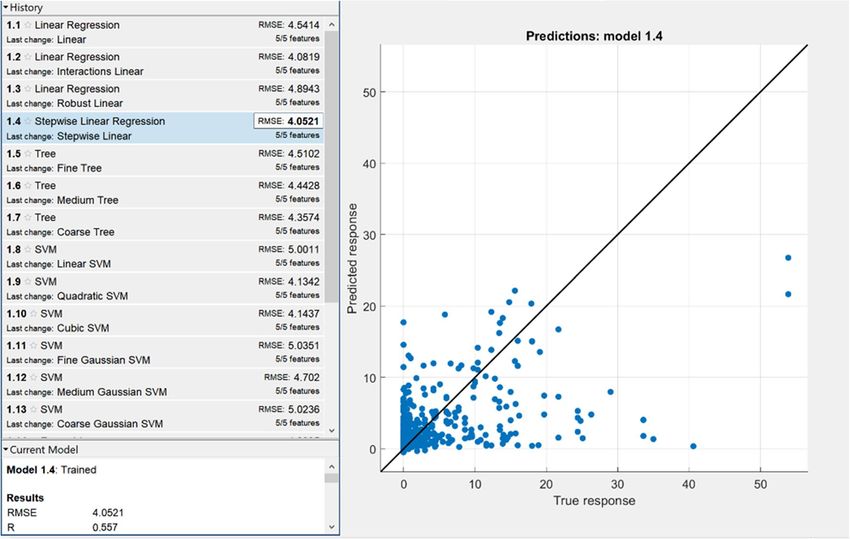
www.nature.com/scientificreports/
Figure 1. Comparison of NWP horizontal resolution model topography of Slovakia: (a) ECMWF; (b)
ALADIN.
• Local NWP models less than 5 km resolution, the forecast horizon is 3 days. Some of the well-known European
models comprise ALADIN (operated in 16 countries) or HIRLAM (operated in 10 countries). As for local
NWP models, the data from global models supply the data for the lateral boundary conditions.
The greater the distance between the grid points, the less likely the model will be capable of discovering small-
scale variations in the temperature and moisture fields. The lack of resolution reduces the amount of detail and
increases the prediction error.
As for local (regional) NWP models, it is characteristic that each country (represented by the national weather
service) calculates the weather forecast individually according to its own computational capacity and needs (e.g.,
some countries can use the ALADIN horizontal resolution 11 km, others have applied the improved version of
resolution of 4.5 km)1. We have identified two major disadvantages of this approach:
• Ineffective searching of weather information from the user’s perspective. There is no common website col-
lecting data from local NWP models. Not all countries make this data open access, so the potential users
must pay for it.
• The national weather agencies must invest a large amount of money to keep their high computing infrastruc-
ture up to date.
On the other hand, several popular web applications collect and visualize data from global models, therefore,
they allow users to find information about the weather conditions for any place. Consequently, we have decided
to calibrate the ECMWF global model by a neural network (hereinafter referred to as NN) to bring 3-day weather
forecast accuracy as close as possible to the selected reference local model ALADIN. Because the 72-hour forecast
period is a standard setting for the ALADIN model, our main objective is to improve ECMWF forecasts to this
time window.
Horizontal resolution can be considered as a major weakness of the ECMWF model. The grid spacing of
9 km means that a geographic area of 81 square kilometres is approximated only by one grid point approaching
the average of the observed values within the grid cell. The region of Central and East Europe consists of several
small countries with a population of less or around 10 million (Slovakia, Czechia, Austria, Slovenia, Hungary,
or Croatia). Due to this fact, the whole area of small and mid-sized cities dominating the settlement structure
of these countries is geographically approximated by one or two topographic points of the ECMWF grid. As a
result of that, the model poorly approximates the terrain and local micro-climate parameters we have recognised
as important weather features, such as green infrastructure or local pollution. These features either exist in the
model initial conditions, but are weakly represented, or are barely incorporated into the model initial condi-
tions. Both situations will impact the forecast. Therefore, after the comprehensive study of the works published,
as well as thanks to the knowledge received from the previous w ork2, we have identified key features that should
effectively replace the main advantage of local NWPs higher resolution. Appropriate features selection helped us
adequately incorporate the influence of small-scale phenomena into the ECMWF forecast, especially in urban
areas.
The main contributions of this paper include the following:
• We describe our approach on improving the accuracy of the ECMWF model based on machine learning
(ML). ML is used for post-processing raw ECMWF data.
• We present a novel perspective of selecting small-scale phenomena that are able to correct a 2 m air tempera-
ture and a 24 h accumulated precipitation forecast error.
• The proposed model can be easily incorporated (open source) into potential online forecast web services;
due to simple model topology, it is robust to overfitting.
Scientific Reports | (2022) 12:7898 | https://doi.org/10.1038/s41598-022-11936-9 2
Vol:.(1234567890)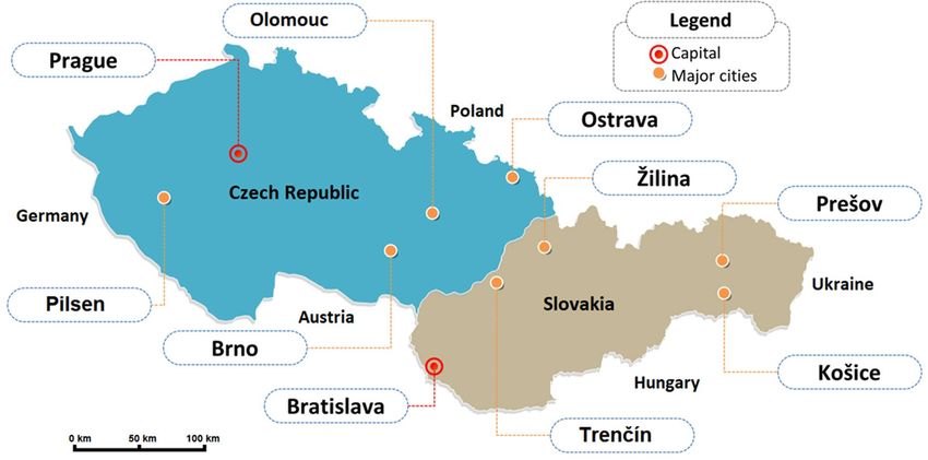
www.nature.com/scientificreports/
The rest of the paper is organised as follows: Section State of the Art reviews some important works in this
research topic. In section Methodology, the details of our hybrid NWP-ML model are presented. Section Results
describes model performance analyses and comparison with the reference local model ALADIN. The benefits
and limitations of the proposed approach are discussed in section Discussion. Summary and future work plans
are presented in section Conclusion.
State of the art
Modern weather prediction systems strongly rely on massive mathematical modelling and simulations which
require high-performance computing. Although we witness a fast increase in computing power, there are still
various challenges in NWP. Regional NWP models need to have accurate information for all forecast variables
and along each model boundary (secured by selected global models), but, due to the unpredictable events in
the atmosphere, even a small change in the initial stage can lead to a huge impact on weather f orecast3. Lower
resolution of global NWP models can take into account even micro-climates such as soil moisture or vegeta-
tion cover, but in a very limited manner. Our suggestion that these parameters are relevant for improving the
accuracy of the forecasts has also been confirmed in the study by Srivastava and B lond4 and Dirmeyer, P. A., and
5
Halder, S. , where the authors proved that the aerosols distribution/concentration and accurate initialization of
soil moisture are both important indicators that can improve air temperature and rainfalls forecasts delivered
by global NWP models. Jhun et al.6, Li et al.7, Perrone et al.8, Requia et al.9, Manso et al.10, Tomson et al.11, Zhao
et al.12, and Schwaab et al.13 have investigated the influence of air pollution as well as the green infrastructure
on weather changes too. Seasonal temperature or precipitation frequency correlates especially on the level of
particulate matter (especially PM2.5). An investigation of the so-called urban heat islands effect brought impor-
tant information on how to improve thermal comfort in urban areas. Green, or sometimes called blue-green,
infrastructure (parks, green walls, wetlands, city forests) help capture pollution and mitigate climate change
(cooling effect, water retention).
The deep neural network is a kind of NN consisting of several layers called hidden layers interconnecting the
vector of input features with the output layer. More layers allow resolving more complex fitting issues and provide
good generalization over the selected dataset. A set of input parameters (features) has to be chosen carefully;
individual parameters should not be cross-correlated. If the NN topology contains many layers and neurons on
each layer, there is a potential risk of overfitting and additional methods for overfitting reduction must be applied.
In the last years, research teams have been increasingly aware of deep learning and trying to use a benefit of it
to improve numerical modelling or apply it for additional post-processing of the delivered NWP forecasts. In
studies by Rasp and Lerch14, Yonekura et al.15, Wang et al.16, Ren et al.17, and Schultz et al.18, the authors tested
the possibility of replacing the traditional forecast model completely by NN or using it for post-processing of
the delivered forecast. While some promising results, that can compete with NWP, have been identified in pilot
models, the research is still in the beginning. A much better situation is in the area of a hybrid approach where
the NWP data are post-processed by NN. Many of the works mentioned focused their attention on the improve-
ment of nowcasting (up to several hours ahead) or a one-day lead. As for heavy rainfalls forecast, in particular,
the authors reached significant accuracy improvement.
We have also contributed to this research. In our pilot work2, we proposed the initial version of our hybrid
model for ECMWF accuracy improvement. We verified that our idea is correct and NN can help improve predic-
tion accuracy. Now, the weather data collected contain three times more samples than we previously used for the
training. We also increased the model’s minimum and maximum forecast range for both the hourly temperature
and the daily precipitations. With respect to the contributions of the above-mentioned works and our knowledge
gained, we changed the NN architecture and replaced two input features. The results obtained are found to be
superior compared to our previous work; and to our best, we have not discovered any model published that
offers ECMWF model accuracy improvement for the 3-day forecasts for both the 2 m air temperature and the
daily precipitation concurrently.
Methodology
At first, we needed to create a large database containing the predicted values of the NWP models selected and
the values measured by weather stations (ground truth). More than one year was spent on collecting the data.
We interrupted gathering the data by the end of February 2020 due to the new coronavirus COVID-19 spreading
across the world. The lockdowns imposed in many countries caused the weather forecasts to be less accurate due
to reduction in aircraft weather r eports19. Had we not interrupted the data collection, we would have received
noisy data. For the short-term forecast, we used open-access data from several web services, namely windy.com
(which uses raw ECMWF data with a 3-hourly step that allows producing forecasts up to 144 h ahead), Yr.no
(operated by Norwegian Meteorological Institute MET; raw ECMWF data with a 1-hour step frequency that
allows a forecast of approximately 60 h ahead; for a longer period forecast, the step increases to 6 h which can
influence total precipitation forecast accuracy for 3rd day) and, finally, the Czech and Slovak Hydrometeorologi-
cal Institutes (both use the ALADIN regional model that is run on their supercomputers)20–23. Weather services in
Czechia and Slovakia also served as sources of real measured values obtained from surface weather observation
stations. All weather stations selected are located near the centre of the following cities (see Table 1 and Fig. 2)
The whole database is composed of 3,679 unique samples. The database was randomly divided into a set
dedicated to the training procedure (90% of samples) and a cross-validation set (10% 368 samples). The data-
base reflects the limitations of the models, such as 3-hour resolution (ECMWF) and maximal 72-hour lead time
(ALADIN). We collected forecasts from all NWP models delivered by forecast run at 00:00 UTC (Coordinated
Universal Time). In the dataset, each date of forecast run (denoted as d) of a particular city is associated with its
Air Quality Index (AQI) of the previous day (d-1) from the website (AQI24).
Scientific Reports | (2022) 12:7898 | https://doi.org/10.1038/s41598-022-11936-9 3
Vol.:(0123456789)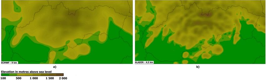
www.nature.com/scientificreports/

                                            City                                   Population       Area [km 2 ]
                                            Prague the capital city of Czechia     1.335 million    496
                                            Brno                                   382,400          230
                                            Ostrava                                285,000          214
                                            Olomouc                                100,500          103
                                            Pilsen                                 175,200          138
                                            Bratislava: Capital city of Slovakia   475,600          368
                                            Zilina                                 81,900           80
                                            Kosice                                 227,500          243
                                            Presov                                 83,900           70
                                            Trencin                                54,500           82

                                           Table 1.  List of selected cities.

                                           Figure 2.  The geographical location of selected cities.

                                            Parameter type                Description
                                            Climatic variables            Hourly surface air temperature, daily precipitation
                                            Weather forecast models       ECMWF, ALADIN, Yr.no
                                            Target data                   Meteorological data from weather stations
                                            Day of forecast               1st, 2nd or 3rd day
                                            Microclimate attributes       MEGI, AQI, water area surface

                                           Table 2.  List of dataset variables.

                                                PM2.5 AQI is calculated according to the PM2.5 level in the air. These matters of size of less than 2.5 µm are
                                           recognized as a major air pollutant with an impact on weather conditions as is stated in section State of the Art.
                                                Green infrastructure has been incorporated in our model via two components, namely the urban water area
                                           surface and the Mean Effective Green Infrastructure (MEGI)25 . The MEGI indicator shows the spatial distribu-
                                           tion of Effective GI, which can be explained as the probability of finding a GI element in a selected urban area.
                                           It is based on circular regions (the distance between two circles is 1 km) around the city centre. Since we col-
                                           lected data from weather stations situated close to the city centres, each city in our database is associated with
                                           the MEGI value reflecting a 5 km distance to the city centre. The list of all dataset variables is shown in Table 2.

                                           Architecture of hybrid NWP/ML prediction model. A neural network based on error back-propaga-
                                           tion comprised an input layer, a hidden layer (one or more) and, finally, an output layer. This topology is inspired
                                           by the learning process of the human brain (creation of new neural connections leads to storing new informa-

          Scientific Reports |   (2022) 12:7898 |                     https://doi.org/10.1038/s41598-022-11936-9                                             4

Vol:.(1234567890)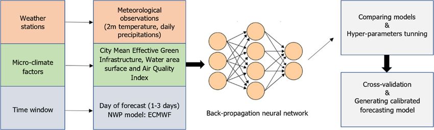
www.nature.com/scientificreports/
Figure 3. The architecture of the proposed model.
tion). The input layer is represented by one or more elements of the input vector called features. The whole
process of NN training and testing is shown in Fig. 3.
Back-propagation neural network is not the only type of neural network. Other well-known types are the
Long Short-Term Memory (LSTM) network or the Convolution Neural Network (CNN). LSTM works with
sequence data such as time series or speech recognition data because the network can store past important
information due to its recurrent connection on the hidden state. Another network CNN applies filters (kernels)
that, by using the convolution operation, allow extracting spatial features e.g., from an image. Therefore, CNN
is good for classification. Because we have tabular data (and create regression model) and, we do not use radar
images or try to predict weather from its previous state, a back-propagation neural network seems to be the best
solution. An example of the input vector x of n-th data sample can be expressed as follows:
Day of forecast 1
AQI 66
xn = MEGI = 15.22
Water area 1.8
ECMWF forecast 14
We tested many topologies, starting from simple networks containing one hidden layer to more sophisticated
topologies consisting of 3 hidden layers, wherein each of them had tens of neurons. To prevent network overfit-
ting, we applied the following techniques:
• Bias Variance Trade-Off: a compromise between the model size and accuracy. A simpler model topology is
preferred.
• Early stopping: training will stop when the preferred performance indicator stops improving on the valida-
tion data subset.
• Bayesian regularization: this method minimizes a combination of squared errors and weights, and then
decides the best combination to create NN that generalizes well.
A model error is considered as a Mean squared error (MSE) defined as follows:
n
1
2
MSE = yi −
yi ,
n
i=1
where n denotes the number of samples and MSE represents the difference between target value yi and output
value (obtained from a trained model) yi i. The root of MSE (RMSE) is a common metric that shows the standard
deviation of residuals (prediction errors) for a particular variable.
A prediction model was implemented in the MATLAB workspace (version 2021a) by using Neural Network
Toolbox which allowed to create testing scripts as well as the so-called MATLAB function of the final version
for further deployment. As an activation function, we used a predefined hyperbolic tangent sigmoid transfer
function (tan-sig). The activation function of each neuron indicates the activation potential of the neuron that
is responsible for the decision whether the node will be fired or not. Tan-sig is an S-shaped curve function that
produces outputs in a scale of [− 1,1]. The non-linearity of this function helps the model to generalize or adjust
better to data diversity.
Results
After the collection of all data, we performed a basic statistical investigation. At first, we analyzed the relative
accuracy of each model prediction outputs. Relative accuracy RA (expressed as a percentage) specifies how
accurate a prediction is when compared to the target value. The formula is expressed as follows:
Scientific Reports | (2022) 12:7898 | https://doi.org/10.1038/s41598-022-11936-9 5
Vol.:(0123456789)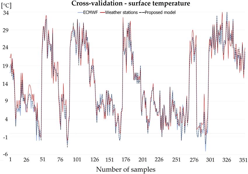
www.nature.com/scientificreports/
Weather model Surface temperature % Daily precipitation %
ALADIN (SHMU and CHMI) 99.7 89.5
Yr (MET) 99.1 86.9
ECMWF (Windy) 97.6 90.8
Table 3. Overview of relative accuracies (RA) of weather prediction models produced for both countries.
Surface temperature Daily precipitation
Weather model − = + − = +
ALADIN (SHMU and CHMI) 42.1% 18.2% 39.7% 15.6% 61.5% 22.9%
Yr (MET) 40.5% 18.3% 41.2% 16.3% 61.2% 22.5%
ECMWF (Windy) 48.3% 18.3% 33.4% 15.7% 60.1% 24.2%
Table 4. Comparison of ratios that determine whether the models’ predictions are overvalued or undervalued.
Note: sign + represents overvaluing,- undervaluing, and = correct prediction.
vt − vt − vp
RA = × 100
vt
where vt denotes the target value and vp represents the predicted value.
Table 3 shows that, in terms of relative accuracy, ECMWF has achieved the worst results of temperature
forecasts, while ALADIN and Yr.no performed equally well (for both models, the RMSE oscillates between 1.25
and 1.5 for the 2 m air temperature). The calculated RA dedicated to the ECMWF 3-day projection is close to
the declared accuracy promoted by ECMWF itself (for year 2019 98%) ( ECMWF26).
An interesting situation occurred when we compared the daily precipitations forecast accuracy, where the
ECMWF model surpassed its two competitors. A detailed analysis related to whether the models overvalue or
undervalue their predictions is another curious fact that we have extracted from the dataset. As it can be seen in
Table 4, in comparison with the other two models, the ECMWF model typically undervalued the temperature
prediction and slightly overvalued the number of daily precipitations.
We can verify this assumption from another point of view. The total number of real measured hourly tem-
peratures above 30 ◦ C is 224. While ALADIN and Yr.no models predicted this warm temperature more than 200
times (concretely ALADIN: 210 and Yr.no: 208), ECMWF estimated that this extreme value would be reached
only 183 times. A relatively high portion of correct predictions of total daily precipitation (more than 60%) can
be explained by a huge number of zero precipitation forecasts that were truly predicted.
Neural network modelling. During the modelling phase, MATLAB allows us to randomly divide the
training set into three subsets, namely a training subset, a validation subset and a testing subset (we chose the
following ratio: 80-10-10). We have applied early stopping which stops the training procedure when the valida-
tion error begins to rise but the training error still decreases in the followings iterations. This event indicates that
the network starts to overfit the data. The trained network is then evaluated on testing data. In case the trained
model performance is adequate for all three subsets, we can use a cross-validation dataset (sometimes referred
to as a holdout) that contains samples not participating in model training.
Figure 4 shows a correlation diagram with the Pearson’s coefficient R for the best-rated topologies, concretely
a hidden layers topology of 7-5-2 for the hourly temperature prediction and an 11-4 for the prediction of total
daily precipitations. Figure 5 compares the proposed model temperature predictions with the raw ECMWF
predictions and with the data observed from weather stations.
Based on the results shown in Table 5, we can say that our proposed hybrid model outperformed raw ECMWF
predictions. For the cross-validation set, by using the RMSE criterion, we have improved the forecast accuracy
by 13% (hourly temperature) and by 45% (daily precipitations).
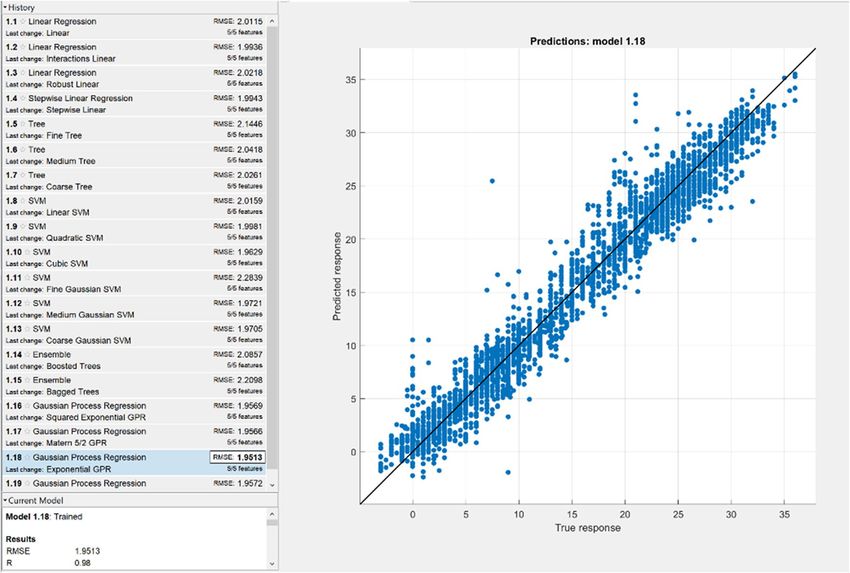
Comparing the performance of different machine learning algorithms. Although NN has been a
trendy ML algorithm in recent days, evaluation of other ML techniques is important to come out with the best-
suited algorithm for a particular issue. MATLAB contains Statistics, and Machine Learning Toolbox allows us to
compare various ML algorithms and build predictive models by automatic training of different regression mod-
els on our data. All available data were used for the training. We set 5-fold cross-validation (good compromise
that saves time and computational complexity (Marcot and Hanea27) to check the models accuracy. Figures 6
and 7 show the results obtained by selected ML algorithms.
As it can be seen in the above-stated figures, performance indicators related to the surface temperature
reach the best values in case of using the Gaussian Process Regression (GPR) model (non-parametric Bayesian
approach). For the total precipitation forecast, Stepwise linear regression becomes the best-assessed model. Based
on these performance measurements, we can say that our proposed ML model outperformed the GPR model (in
Scientific Reports | (2022) 12:7898 | https://doi.org/10.1038/s41598-022-11936-9 6
Vol:.(1234567890)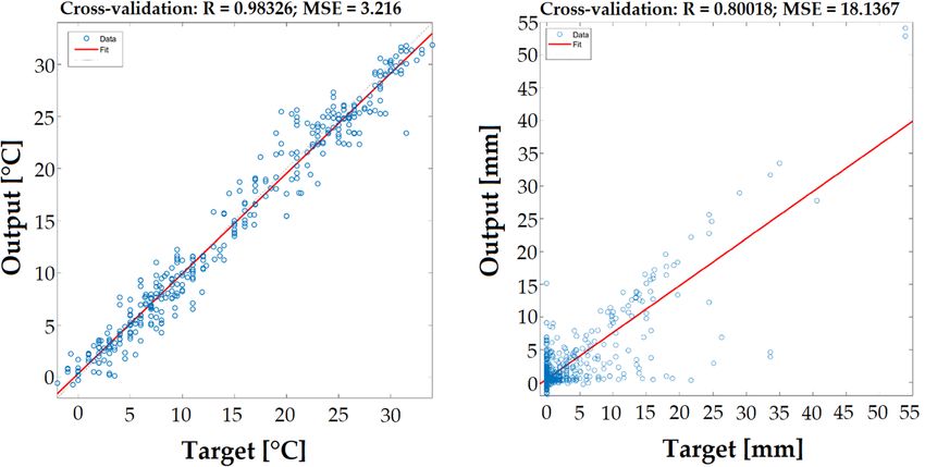
www.nature.com/scientificreports/

                                 Figure 4.  Scatter plot with the Pearsons correlation coefficient R and MSE of hourly temperature prediction in
                                 the left part and daily precipitation prediction in the right part.

                                 Figure 5.  Comparison of predicted surface temperature from the proposed model and ECMWF, and reference
                                 temperature from weather stations.

                                 a form of R as well as RMSE for both cases training and cross-validation). In total daily precipitation prediction,
                                 our model achieved better results on the training data (and significantly better R value in cross-validation). The
                                 RMSE metric in cross-validation where we received slightly worse outcome (4.26 vs 4.05, 5% difference between
                                 the models performance) was the only exception. On the other hand, it needs to be considered that these ML
                                 techniques used all available data; before NN training, the dataset was divided into training and cross-validation
                                 (independent) data subsets.
                                     Therefore, we have enough information to assess our model truly. Based on these measurements, we can
                                 say that the back-propagation neural network selected is the best fit model (for non-linear mapping) with the
                                 highest prediction accuracy.

Scientific Reports |   (2022) 12:7898 |               https://doi.org/10.1038/s41598-022-11936-9                                                   7

                                                                                                                                             Vol.:(0123456789)
www.nature.com/scientificreports/
Surface Daily
temperature precipitation
Weather model MSE RMSE MSE RMSE
ECMWF 4.44 2.11 °C 42.28 6.5 mm
Proposed model 3.73 1.93 °C 11.49 3.39 mm
Cross-validation set
ECMWF 4.09 2.02 °C 38.17 6.18 mm
Proposed model 3.22 1.79 °C 18.14 4.26 mm
Table 5. Proposed model performance evaluation.
Figure 6. Correlation diagram of selected ML models (RMSE and Pearsons correlation coefficient R) for hourly
temperature prediction.
Discussion
We have prepared a hybrid deep learning model able to correct ECMWF short-time forecasts (up to 3 days
ahead). The proposed model significantly extends the pilot study published in 2019 (an increase of forecast
ranges from 15 °C − 35 °C to −5 °C − 35 °C; and 24 h precipitation forecast modelling starts from 0 mm instead
of 2 mm). The key performance indicator RMSE is also better compared to the pilot study (2.06 C and 3.68 mm
the training set of the pilot model). We also acquired three times more unique data samples available for train-
ing and testing. As shown in Table 5, the proposed model improved the prediction ability of the raw ECMWF
model. The proposed model is comprised of simple NN architecture which implies good generalizing ability
and robustness to overfitting. The model is easy to integrate as a post-processing approach for ECMWF outputs.
Table 5 also shows that the results obtained for the model during the training and cross-validation are generally
consistent and MSE falls close to the values represented by the local NWP model. A combination of deep learn-
ing and global NWP outcome can offer similar prediction accuracy as the local model.
We should consider and discuss the limitations of this study. Zero precipitation rate accounts for more than
66% of all data. There is a noticeable imbalance in the data, and all papers mentioned here had to find methods
to effectively handle imbalanced datasets. An imbalanced dataset may have a negative impact on the performance
of machine learning, especially as for classification models. Thus, our primary goal was to adapt the model itself
by hyper-parameter tuning and monitoring feedback from metrics. We also adopted a strategy described by Liu
et al.28 to deal with this issue. The precipitation training dataset was a combination of randomly chosen data
from a non-rainfall subset as well as from a rainfall data subset. The proportion of occurrence of data extracted
Scientific Reports | (2022) 12:7898 | https://doi.org/10.1038/s41598-022-11936-9 8
Vol:.(1234567890)www.nature.com/scientificreports/
Figure 7. Correlation diagram of selected ML models (RMSE and Pearsons correlation coefficient R) of daily
precipitation prediction.
from these two subsets is 1:1. This special training dataset was used for the training NN (we used only 1,129
data samples in this case).
Another fact that we must consider is that the daily precipitation summary is valid for a period from midnight
to midnight. A situation may occur when rain is expected e.g., at 22:00, but the rainfall starts after midnight. Only
a few hours delay will affect the predictive accuracy for the actual and following days of the forecast. Finally, the
temperature prediction range represents a drawback of the proposed model. Due to the relatively warm winter,
we have recorded hourly temperatures below minus 5 degrees of Celsius only a few times. There is no doubt that,
in many countries, the lowest temperature during winter is much lower than the actual model offers. Unfortu-
nately, we must wait until the situation with air traffic returns to its pre-COVID levels, and, then, we can focus
on gathering data with low surface temperature to improve the prediction range of our model.
It is not easy to find research papers for comparison. Many authors have turned their attention to improve-
ment of the prediction accuracy for nowcasting (up to next 12 h) or extreme weather phenomena such as rainfalls
or monsoons. Nevertheless, we have found several interesting articles. Li et al29 tested linear and Random Forest
algorithms to improve the ECMWF forecast in the Beijing area. They gathered data during the period between
2012 and 2016. The proposed model increases accuracy by 9.61% compared to the ECMWF for surface tempera-
ture prediction. Another group of Chinese researchers in Kong et al.30 created a model for a weather conditions
forecast for the upcoming 3 days. They gathered historical observational data from 226 weather stations across
Beijing between 2015 and 2017. The proposed model was based on the convolutional neural network containing
44 forecast predictors. While the ECMWF model reached RMSE of 2.94, their trained model reduced the error to
2.41 in temperature forecasting. In Thi Kieu Tran et al.31, the authors tested three machine learning algorithms. In
addition to NN, they also used the recurrent neural network (RNN) and LSTM. According to the season of the
year, RMSE oscillated between 2.52 and 3.65 ◦ C in the data test of the daily maximum temperature prediction
for the upcoming 3 days. Error comparison with the data observed is missing.
In ECMWF technical memorandum number 89632, authors analyzed three machine learning algorithms
(linear regression, random forests, and NN) for statistical modelling of 2 m temperature and 10 m wind speed
forecast errors. Compared to our model, their corrected model produced a forecast with a lead time up to only
48 h and their models’ configurations often used more than 10 predictors (features). RMSE was reduced by
around 10%. NN model outputs were slightly better than the other two mentioned methods, its RMSE oscillates
between 1.9 and 2.4 ◦ for 48 h forecast lead time.
Better short-term precipitation prediction from radar echo images was the main contribution of the paper
by Niu et al.33, where the authors used a combination of multi-channel ConvLSTM and 3D-CNN algorithms.
Based on the data collected between 2017 and 2018, their model achieved an RMSE value of 7.18 mm. The
preprint paper by Chen and W ang34 describes an application of DL in a short-term precipitation prediction (fol-
lowing 24 h). The proposed model reached smaller RMSE (4.16 mm/24 h) than the ERA-Interim 24 h forecast
(4.78 mm/24 h) that estimates the global atmospheric state based on the data from ECMWF. Saminathan et al.35
calibrated the delivered precipitation forecast provided by Global Ensemble Forecast System (GEFS) over the
Scientific Reports | (2022) 12:7898 | https://doi.org/10.1038/s41598-022-11936-9 9
Vol.:(0123456789)www.nature.com/scientificreports/
Indian region. They used NN as a post-processing technique for forecast enhancement. The prediction error
represented by RMSE was improved from 9.8 to 9.1 for a 3-day lead. Finally, Rasel et al.36 tested ML models based
on Support Vector Regression (SVR) and NN for weather forecast accuracy improvement for a time period of one
week. In terms of RMSE, the best models with a low error rate included SVR (with its value of 21.68 mm/24 h)
and NN (with an error rate of 7.89 ◦C).
Based on the above-mentioned papers published, it is obvious that the combination of temperature and
precipitation forecast accuracy improvement is unique in this research field. In addition, our paper brings a
calibration model that can be easily incorporated into popular online weather services.
Conclusions
This paper proposes ECMWF model calibration based on DL. The novelty of this approach lies in prediction
accuracy improvement for both 2 m air temperature and daily precipitation in a 3-day lead. Performance analysis
of our model pointed out an error (RMSE) reduction by 13% (2 m air temperature) and 45% (24 h precipita-
tion) respectively. In comparison to regional NWP models, the global model ECMWF has no geographical
restrictions in forecasts provided, thus it is more attractive for both professionals and basic users. It is also worth
mentioning that our approach could potentially reduce the acquisition costs of supercomputers. For example,
in 2018, the Czech hydrometeorological institute bought a supercomputer with a theoretical peak performance
of 270 Teraflops (NEC LX-Series x86 with 320 nodes). On the other hand, we tested our model on PC Intel(R)
Core(TM) i7-9700 CPU @ 3.00 GHz with 16 GB RAM, and the corrected ECMWF predictions were calculated
in the MATLAB environment almost immediately ( CHMI21). In future work, we plan to extend the calibrated
forecast period and incorporate another weather phenomenon the wind speed.
Data availability
The data sets source code of proposed models are available online in Zenodo repository (https://doi.org/10.5281/
zenodo.5862250). The air quality and meteorological data used in this work are public and freely available from
ECMWF, Yr.no, SHMU, CHMI, and AQI.
Received: 16 March 2022; Accepted: 3 May 2022
References
1. Belluš, M. et al. Aire limitée adaptation dynamique développement InterNational—limited area ensemble forecasting (ALADIN-
LAEF). Adv. Sci. Res. 16, 63–68. https://doi.org/10.5194/asr-16-63-2019 (2019).
2. Frnda, J. et al. A weather forecast model accuracy analysis and ECMWF enhancement proposal by neural network. Sensors 19,
5144. https://doi.org/10.3390/s19235144 (2019).
3. Bisták, A., Hulínová, Z., Neštiak, M. & Chamulová, B. Simulation modeling of aerial work completed by helicopters in the con-
struction industry focused on weather conditions. Sustainability 13, 13671. https://doi.org/10.3390/su132413671 (2021).
4. Srivastava, N. & Blond, N. Impact of meteorological parameterization schemes on CTM model simulations. Atmos. Environ.https://
doi.org/10.1016/j.atmosenv.2021.118832 (2022).
5. Dirmeyer, P. A. & Halder, S. Sensitivity of numerical weather forecasts to initial soil moisture variations in CFSv2. Weather Forecast.
31, 1973–1983. https://doi.org/10.1175/waf-d-16-0049.1 (2016).
6. Jhun, I., Coull, B. A., Schwartz, J., Hubbell, B. & Koutrakis, P. The impact of weather changes on air quality and health in the united
states in 1994–2012. Environ. Res. Lett.https://doi.org/10.1088/1748-9326/10/8/084009 (2015).
7. Li, X.-X., Koh, T.-Y., Panda, J. & Norford, L. K. Impact of urbanization patterns on the local climate of a tropical city, Singapore:
an ensemble study. J. Geophys. Res. Atmos. 121, 4386–4403. https://doi.org/10.1002/2015jd024452 (2016).
8. Perrone, M. R. et al. Weekly cycle assessment of PM mass concentrations and sources, and impacts on temperature and wind speed
in Southern Italy. Atmos. Res. 218, 129–144. https://doi.org/10.1016/j.atmosres.2018.11.013 (2019).
9. Requia, W. J., Jhun, I., Coull, B. A. & Koutrakis, P. Climate impact on ambient PM2.5 elemental concentration in the united states:
a trend analysis over the last 30 years. Environ. Int.https://doi.org/10.1016/j.envint.2019.05.082 (2019).
10. Manso, M., Teotónio, I., Silva, C. M. & Cruz, C. O. Green roof and green wall benefits and costs: a review of the quantitative
evidence. Renew. Sustain. Energy Rev.https://doi.org/10.1016/j.rser.2020.110111 (2021).
11. Tomson, M. et al. Green infrastructure for air quality improvement in street canyons. Environ. Int. 146, 106288. https://doi.org/
10.1016/j.envint.2020.106288 (2021).
12. Zhao, D. et al. The impact threshold of the aerosol radiative forcing on the boundary layer structure in the pollution region. Atmos.
Chem. Phys. 21, 5739–5753. https://doi.org/10.5194/acp-21-5739-2021 (2021).
13. Schwaab, J. et al. The role of urban trees in reducing land surface temperatures in European cities. Nat. Commun.https://doi.org/
10.1038/s41467-021-26768-w (2021).
14. Rasp, S. & Lerch, S. Neural networks for postprocessing ensemble weather forecasts. Mon. Weather Rev. 146, 3885–3900. https://
doi.org/10.1175/mwr-d-18-0187.1 (2018).
15. Yonekura, K., Hattori, H. & Suzuki, T. Short-term local weather forecast using dense weather station by deep neural network. In
2018 IEEE International Conference on Big Data (Big Data), https://doi.org/10.1109/bigdata.2018.8622195 (IEEE, 2018).
16. Wang, B. et al. Deep uncertainty quantification. In Proceedings of the 25th ACM SIGKDD International Conference on Knowledge
Discovery & Data Mining, https://doi.org/10.1145/3292500.3330704 (ACM, 2019).
17. Ren, X. et al. Deep learning-based weather prediction: a survey. Big Data Res.https://doi.org/10.1016/j.bdr.2020.100178 (2021).
18. Schultz, M. G. et al. Can deep learning beat numerical weather prediction?. Philos. Trans. R. Soc. A Math. Phys. Eng. Sci. 379,
20200097. https://doi.org/10.1098/rsta.2020.0097 (2021).
19. Chen, Y. COVID-19 pandemic imperils weather forecast. Geophys. Res. Lett.https://doi.org/10.1029/2020gl088613 (2020).
20. Slavovsky, T. Windy. https://www.ecmwf.int/en/elibrary/17309-windy, (2017).
21. CHMI. Czech hydrometeorological institute. https://www.chmi.cz/?l=en, (2022).
22. SHMU. Slovak hydrometeorological institute. https://www.shmu.sk/en/, (2022).
23. YR.No. Forecast data model. https://developer.yr.no/doc/locationforecast/datamodel/, (2022).
24. AQI air pollution: real-time air quality index. https://aqicn.org, (2022).
25. UGI. Urban green infrastructure. https://eea.maps.arcgis.com/apps/MapSeries/index.html?appid=42bf8cc04ebd49908534efde0
4c4eec8%20&embed=true, (2022).
Scientific Reports | (2022) 12:7898 | https://doi.org/10.1038/s41598-022-11936-9 10
Vol:.(1234567890)www.nature.com/scientificreports/
26. ECMWF. Anomaly correlation of ECMWF 500 hpa height forecasts. https://www.ecmwf.int/en/forecasts/charts/catalogue/
plwww_m_hr_ccaf_adrian_ts?facets=undefi ned&time=2022011100, (2022).
27. Marcot, B. G. & Hanea, A. M. What is an optimal value of k in k-fold cross-validation in discrete Bayesian network analysis?.
Comput. Stat. 36, 2009–2031. https://doi.org/10.1007/s00180-020-00999-9 (2020).
28. Liu, Y. et al. Short-term rainfall forecast model based on the improved BP–NN algorithm. Sci. Rep.https://doi.org/10.1038/s41598-
019-56452-5 (2019).
29. Li, H. et al. A model output machine learning method for grid temperature forecasts in the Beijing area. Adv. Atmos. Sci. 36,
1156–1170. https://doi.org/10.1007/s00376-019-9023-z (2019).
30. Kong, W. A deep spatio-temporal forecasting model for multi-site weather prediction post-processing. Commun. Comput. Phys.
31, 131–153. https://doi.org/10.4208/cicp.oa-2020-0158 (2022).
31. Tran, T. T. K., Lee, T., Shin, J.-Y., Kim, J.-S. & Kamruzzaman, M. Deep learning-based maximum temperature forecasting assisted
with meta-learning for hyperparameter optimization. Atmosphere 11, 487. https://doi.org/10.3390/atmos11050487 (2020).
32. Ben-Bouallegue, Z. et al. Statistical modelling of 2m temperature and 10m wind speed forecast errors. ECMWF Technical Memo-
randahttps://doi.org/10.21957/VDCCCJA3F (2022).
33. Niu, D. et al. Precipitation forecast based on multi-channel ConvLSTM and 3d-CNN. In 2020 International Conference on
Unmanned Aircraft Systems (ICUAS), https://doi.org/10.1109/icuas48674.2020.9213930 (IEEE, 2020).
34. Chen, G. & Wang, W.-C. Short-term precipitation prediction using deep learning. arXiv:2110.01843 (2021).
35. Saminathan, S., Medina, H., Mitra, S. & Tian, D. Improving short to medium range GEFS precipitation forecast in India. J.
Hydrol.https://doi.org/10.1016/j.jhydrol.2021.126431 (2021).
36. Rasel, R. I., Sultana, N. & Meesad, P. An application of data mining and machine learning for weather forecasting. In Meesad, P.,
Sodsee, S., Unger, H. (eds) Recent Advances in Information and Communication Technology 2017. IC2IT 2017. Advances in Intel-
ligent Systems and Computing, vol. 566, https://doi.org/10.1007/978-3-319-60663-7_16 (Springer, Cham, 2018).
Acknowledgements
This research was funded by Slovak Grant Agency for Science (VEGA) under Grant No. 1/0157/21 and partially
supported by Grant System of University of Zilina no. 1/2021 (12766) and by the VSB-Technical University of
Ostrava, the Ministry of Education, Youth and Sports, Czech Republic, under Grant SP2022/5 and SP2022/18.
Author contributions
Conceptualization, J.F. and M.D.; methodology, J.F., M.D., M.V. and J.R.; software, J.F., J.N. and R.M. validation,
J.F., M.D., and J.R.; formal analysis, J.R., J.N. and R.M.; resources, J.F. and M.V.; data curation, M.D. and J.R.;
writing original draft preparation, J.F.; writing review and editing, M.D., J.R. and J.N.; visualization, J.F and J.N.;
supervision, R.M. and J.R.; project administration, J.F. and M.D.; funding acquisition, J.F. All authors have read
and agreed to the published version of the manuscript.
Competing interests
The authors declare no competing interests.
Additional information
Correspondence and requests for materials should be addressed to J.F.
Reprints and permissions information is available at www.nature.com/reprints.
Publisher’s note Springer Nature remains neutral with regard to jurisdictional claims in published maps and
institutional affiliations.
Open Access This article is licensed under a Creative Commons Attribution 4.0 International
License, which permits use, sharing, adaptation, distribution and reproduction in any medium or
format, as long as you give appropriate credit to the original author(s) and the source, provide a link to the
Creative Commons licence, and indicate if changes were made. The images or other third party material in this
article are included in the article’s Creative Commons licence, unless indicated otherwise in a credit line to the
material. If material is not included in the article’s Creative Commons licence and your intended use is not
permitted by statutory regulation or exceeds the permitted use, you will need to obtain permission directly from
the copyright holder. To view a copy of this licence, visit http://creativecommons.org/licenses/by/4.0/.
© The Author(s) 2022
Scientific Reports | (2022) 12:7898 | https://doi.org/10.1038/s41598-022-11936-9 11
Vol.:(0123456789)You can also read