Magnetic and tidal migration of close-in planets
←
→
Page content transcription
If your browser does not render page correctly, please read the page content below
Astronomy & Astrophysics manuscript no. aanda                                                                                         ©ESO 2021
                                               April 19, 2021

                                                                   Magnetic and tidal migration of close-in planets
                                                                          Influence of secular evolution on their population
                                                                                       J. Ahuir1 , A. Strugarek1 , A.-S. Brun1 and S. Mathis1

                                                    Département d’Astrophysique-AIM, CEA/DRF/IRFU, CNRS/INSU, Université Paris-Saclay, Université de Paris, F-91191 Gif-sur-
                                                    Yvette, France
                                                    e-mail: jeremy.ahuir@cea.fr

                                                    Received XXX; accepted XXX
arXiv:2104.01004v2 [astro-ph.EP] 16 Apr 2021

                                                                                                                  ABSTRACT

                                                    Context. Over the last two decades, a large population of close-in planets has been detected around a wide variety of host stars. Such
                                                    exoplanets are likely to undergo planetary migration through magnetic and tidal interactions.
                                                    Aims. We aim to follow the orbital evolution of a planet along the structural and rotational evolution of its host star, simultaneously
                                                    taking into account tidal and magnetic torques, in order to explain some properties of the distribution of observed close-in planets.
                                                    Methods. We rely on a numerical model of a coplanar circular star–planet system called ESPEM, which takes into account stellar
                                                    structural changes, wind braking, and star–planet interactions. We browse the parameter space of the star–planet system configurations
                                                    and assess the relative influence of magnetic and tidal torques on its secular evolution. We then synthesize star–planet populations and
                                                    compare their distribution in orbital and stellar rotation periods to Kepler satellite data.
                                                    Results. Magnetic and tidal interactions act together on planetary migration and stellar rotation. Furthermore, both interactions can
                                                    dominate secular evolution depending on the initial configuration of the system and the evolutionary phase considered. Indeed, tidal
                                                    effects tend to dominate for high stellar and planetary masses as well as low semi-major axis; they also govern the evolution of planets
                                                    orbiting fast rotators while slower rotators evolve essentially through magnetic interactions. Moreover, three populations of star–
                                                    planet systems emerge from the combined action of both kinds of interactions. First, systems undergoing negligible migration define
                                                    an area of influence of star–planet interactions. For sufficiently large planetary magnetic fields, the magnetic torque determines the
                                                    extension of this region. Next, planets close to fast rotators migrate efficiently during the pre-main sequence (PMS), which engenders
                                                    a depleted region at low rotation and orbital periods. Then, the migration of planets close to slower rotators, which happens during the
                                                    main sequence (MS), may lead to a break in gyrochronology for high stellar and planetary masses. This also creates a region at high
                                                    rotation periods and low orbital periods not populated by star–planet systems. We also find that star–planet interactions significantly
                                                    impact the global distribution in orbital periods by depleting more planets for higher planetary masses and planetary magnetic fields.
                                                    However, the global distribution in stellar rotation periods is marginally affected, as around 0.5 % of G-type stars and 0.1 % of
                                                    K-type stars may spin up because of planetary engulfment. More precisely, star–planet magnetic interactions significantly affect the
                                                    distribution of super-Earths around stars with a rotation period higher than around 5 days, which improves the agreement between
                                                    synthetic populations and observations at orbital periods of less than 1 day. Tidal effects for their part shape the distribution of giant
                                                    planets.
                                                    Key words. planet-star interactions – stars: evolution – stars: solar-type – stars: rotation

                                               1. Introduction                                                            of these interactions may have been identified in individual sys-
                                                                                                                          tems (e.g., HD 189733 ; see Dowling Jones et al. 2018; Cauley
                                               Since the detection of 51 Pegasi b by Mayor & Queloz (1995),               et al. 2018) as well as in the distribution of some planetary pop-
                                               more than 4000 exoplanets have been detected. The observed                 ulations. More precisely, McQuillan et al. (2013) estimated the
                                               populations show a wide variety of host stars, orbital architec-           rotation period of 737 stars hosting Kepler objects of interest us-
                                               tures, planetary sizes, and masses. Moreover, because of the bi-           ing an auto-correlation method, and identified a possible dearth
                                               ases of the most successful detection methods, namely, the tran-           of planets with orbital periods shorter than 2-3 days around fast
                                               sit and radial velocity techniques, a majority of the discovered           rotators (with a rotation period shorter than 10 days). Teitler &
                                               planets orbit close to their host stars, whether they are of mass          Königl (2014) first proposed that such a phenomenon may be at-
                                               comparable to that of Jupiter (forming the population of hot               tributed to the engulfment of close-in planets by their host stars
                                               Jupiters, e.g., Mayor & Queloz 1995; Henry et al. 2000; Char-              through tidal interactions. Lanza & Shkolnik (2014) suggested
                                               bonneau et al. 2000) or slightly larger than that of the Earth (the        an alternative scenario based on secular perturbations in multi-
                                               so-called super-Earths, such as 55 Cnc e; see Dawson & Fab-                planet systems. These latter authors showed that remote plan-
                                               rycky 2010). Close-in planets orbit in a dense and magnetized              ets which are excited on a sufficiently eccentric orbit around old
                                               medium, which leads to the emergence of star–planet interac-               stars may be tidally circularized on shorter orbits. Furthermore,
                                               tions that can affect the dynamics and evolution of the orbital            Walkowicz & Basri (2013) found a concentration of massive
                                               systems (Cuntz et al. 2000). In particular, angular momentum               planets with an orbital period equal to either the rotation period
                                               exchanges can occur between the planetary orbit and the stel-              of their host star or half that period, which could be the signature
                                               lar spin, leading to migration of the planet. Potential signatures
                                                                                                                                                                      Article number, page 1 of 28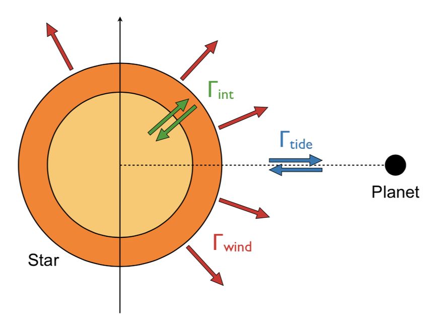
A&A proofs: manuscript no. aanda

of tidal interactions. In view of these different aspects, under-        tude, and is at the origin of an exchange of angular momentum
standing how compact systems form and evolve is a key astro-             between the star and the planet. Indeed, a net tidal torque is ap-
physical question to be addressed.                                       plied both on the planetary orbit and on stellar rotation to reduce
     The role of the protoplanetary disk in shaping the observed         the angle δ. The position of the planet with respect to the co-
structure of planetary systems is strongly emphasized in the             rotation radius (for which n = Ω? , see the black dashed line in
literature. Indeed, the disk structure and evolution have a sig-         Fig. 1) then determines the evolution of the system. If the planet
nificant influence on the mass and semi-major axis distribution          is situated beyond this characteristic distance, an outward mi-
of the young planets (e.g., Mordasini, Alibert & Benz 2009;              gration makes it move away from the host star, which then spins
Mordasini et al. 2009). In particular, planet migration in the disk      down. Otherwise the planet migrates inward, moving closer to
through Lindblad resonances is thought to be efficient in shaping        the spinning-up star. In the latter case, the fate of the system is
planetary systems (Baruteau et al. 2014; Bouvier & Cébron                determined by the orbital angular momentum Lorb of the planet
2015; Heller 2019). Moreover, population synthesis models                and the stellar angular momentum L? : if Lorb ≥ 3L? , an equilib-
have been developed to better understand the interplay between           rium state is reached where the angular velocities Ω? and n are
the properties of the disk and the different processes shaping           synchronized. Otherwise, the planet migrates too efficiently and
planetary systems (we refer the reader to Mordasini 2018,                it spirals towards its host star until its disruption at the Roche
for an extended review). The predicted distributions were then           limit (Hut 1980, 1981). It is important to note that such a condi-
compared to Kepler observations in order to constrain models             tion is based on the conservation of the total angular momentum
of planetary formation and evolution (Mulders et al. 2019).              of the star–planet system. Damiani & Lanza (2015) derived a
For a large range of multi-planet system properties (e.g., orbital       similar criterion by taking into account magnetic braking. More
period ratios, mutual inclination, position of the innermost             generally, to provide a realistic and complete equilibrium crite-
planet), these synthetic populations are in good agreement with          rion, it is necessary to take into account magnetic braking, an-
Kepler global distributions, if multiple interacting seed planet         gular momentum redistribution within the star, and the various
cores per disk are taken into account.                                   star–planet interactions simultaneously.
                                                                              Tidal interactions are modulated by the structural and rota-
    After the dissipation of the disk, dynamical interactions,           tional evolution of the star. The stellar rotation rate generally
in particular Kozai oscillations, may occur in multiplanet sys-          exhibits a complex evolution due to the initial disk–star inter-
tems, leading to an intricate evolution of their orbital architec-       action, the internal redistribution of angular momentum within
ture (Laskar et al. 2012; Bolmont et al. 2015). However, iso-            the star during contraction phases, and the angular momentum
lated close-in planets can already suffer efficient migration be-        extraction by the stellar wind (e.g. Weber & Davis 1967; Sku-
cause of magnetic and tidal interactions with their host star. We        manich 1972; Kawaler 1988; Matt et al. 2012; Réville et. al.
consider this simpler case in the present work, where we aim             2015a). As this intricacy may significantly affect the evolution of
to account for the variety of such star–planet interactions. We          a given star–planet system, it is necessary to take such processes
therefore consider a simplified system comprising a star and a           into account as much as possible. This requires models cali-
single planet on a circular orbit perpendicular to the stellar ro-       brated on gyrochronology and rotational distributions in open
tation axis. One of the main physical processes acting in such a         clusters (Gallet & Bouvier 2015; Matt et al. 2015), leading up to
configuration are tidal interactions. These result from the gravi-       general frameworks combining stellar rotation, wind, and mag-
tational response of a star to the presence of a planet and play a       netism (Johnstone et al. 2015a; Ahuir et al. 2020). Past studies
key role in the evolution of the orbital configuration of the sys-       have taken these constraints into account to some extent. For in-
tem. Two components arise from the stellar response: the hy-             stance, Zhang & Penev (2014) relied on the two-layer rotational
drostatic nonwavelike equilibrium tide, dissipated by turbulent          model of MacGregor & Brenner (1991) and a constant tidal dis-
friction (Zahn 1966; Remus et al. 2012; Ogilvie 2013), and the           sipation to deal with the secular evolution of star–planet systems,
dynamical tide, which consists in the excitation of waves inside         and subsequently adopted a statistical approach to their numeri-
the star by the tidal potential as well as their dissipation. A dy-      cal simulations in order to apply constrains to tidal theory. Bol-
namical tide can exist in both radiative zones (through internal         mont & Mathis (2016) then first incorporated the effects of dy-
gravity waves, Zahn 1975; Goldreich & Nicholson 1989; Good-              namical tide in stellar convection zones and studied their impact
man & Dickson 1998; Terquem et al. 1998) and convective                  on the secular evolution of star–planet systems by considering
zones (Ogilvie & Lin 2007; Ogilvie 2013; Mathis 2015). We                a one-layer rotational model for the central star. More recently,
focus on the latter in this study and leave a detailed investigation     Benbakoura et al. (2019) performed a study based on the amal-
of internal gravity waves to future work (Barker 2020; Ahuir,            gamation of the two previous studies, taking a bi-layer structure
Mathis & Amard 2021). In the stellar convective zone, if the or-         for the star and both the equilibrium and dynamical tides into
bital period of the planet is longer than half of the stellar rotation   account. This allowed them to provide a criterion for planetary
period, inertial waves restored by the Coriolis force are excited        engulfment due to tidal effects, taking into account stellar evo-
and dissipated in the envelope of solar-type stars. Otherwise, in-       lution. They were also able to characterize the influence of such
ertial waves cannot be excited and no dynamical tide is raised           a phenomena on the rotation of the host star. In parallel, Gallet
in the star (see the violet area in Fig. 1). The associated dissipa-     et al. (2018) and Gallet & Delorme (2019) relied on a similar
tion, which depends on stellar internal structure as it arises from      model to investigate the rotational evolution of planet-hosting
the reflection of the waves on the radiative core (Ogilvie 2013;         stars in open clusters (in particular in the Pleiades) in more de-
Goodman & Lackner 2009; Mathis 2015), can be several or-                 tail, which allowed them to assess some limits of gyrochronol-
ders of magnitude higher than the dissipation of the equilibrium         ogy (Barnes 2003). Finally, the evolution of star–planets system
tide (Ogilvie & Lin 2007; Bolmont & Mathis 2016). When tidal             under tidal interactions during the red giant phase has also been
dissipation is taken into account, the stellar response presents a       extensively investigated (Privitera et al. 2016a,b; Meynet et al.
delay and the associated bulge is misaligned with the line joining       2017; Rao et al. 2018).
the centers of the two celestial bodies. This misalignment then               However, in past studies, tidal effects and magnetism have
induces a lag angle δ, which increases with dissipation magni-           not been taken into account together systematically (apart from
Article number, page 2 of 28
J. Ahuir , A. Strugarek , A.-S. Brun and S. Mathis : Magnetic and tidal migration of close-in planets
Ω
Star
n > 2Ω Planetary orbit Co-rotation Alfvén radius
δ
Equilibrium tide
only Inward
n
Outward
Alfvén Planet
wings
Stellar wind
lanet
le star-p ns
Negligib te r ac tio
c in
magneti
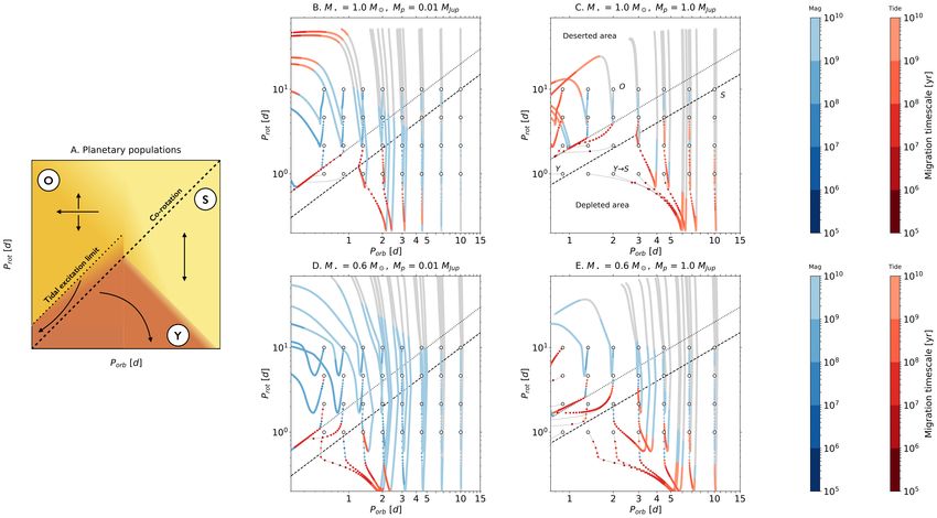
Fig. 1. Sketch of the main features and locations of interest involved in a star–planet system undergoing tidal and magnetic interactions. The
planet (in blue) orbits the star (in orange) with an orbital angular velocity n. As a result of the presence of a planet, the star presents a bulge
misaligned with the line joining the centers of the two celestial bodies, which induces a lag angle δ. This angle has been greatly exaggerated here
for visualization purposes (it is indeed much smaller than 1 degree in almost all cases). If the planetary mean motion is greater than twice the stellar
rotation rate, inertial waves cannot be excited in the stellar convective zone and no dynamical tide is raised within the convective envelope of the
star (see the purple area). The relative motion between the planet and the ambient wind (represented with orange arrows) leads to the formation
of Alfvén wings (orange lobes around the planet) if the planet is below the Alfvén radius (in blue). Beyond this distance, no Alfvén wings can
connect the star and the planet (see the gray area). For both tidal and magnetic interactions, a planet situated below the co-rotation radius (see
the black dashed line) undergoes an inward migration, and a planet situated beyond this distance migrates outwards. The relative position of the
different orbits of interest may vary depending on the initial configuration of the system considered.
wind braking). Bouvier & Cébron (2015) first explored the pos- a determining role in planetary migration in both cases. Many
sibility that tidal and magnetic interactions may compete with other notable effects, such as anomalous emissions or planet in-
accretion and contraction in the case of a close-in planet em- flation, may result from star–planet magnetic interactions (we re-
bedded in a disk. Furthermore, after the dissipation of the lat- fer the reader to Lanza 2018, for a recent review). Strugarek et
ter, star–planet magnetic interactions may occur because of the al. (2017) performed a first study on planetary migration taking
relative motion between the planet and the ambient wind at the into account tidal and magnetic torques simultaneously. In par-
planetary orbit (represented with orange arrows in Fig. 1). If the ticular, they computed the migration timescale of the planet for
planet is below the Alfvén radius (at which the wind velocity both contributions, finding that both effects could play a key role
is equal to the local Alfven speed; see the blue line in Fig. 1), depending on the characteristics of the star–planet system con-
the magnetic torque applied to the planet can lead to efficient sidered. Thus, following the orbital evolution of a planet along
transport of angular momentum between the planet and the star the rotational and structural evolution of the host star by taking
through the so-called Alfvén wings (Neubauer 1998, see the or- into account the coupled effects of tidal and magnetic torques is
ange lobes around the planet in Fig. 1). Beyond the Alfvén ra- essential to better understanding the evolution of star–planet sys-
dius, the wind becomes superalfvénic. In this case, Alfvén wings tems. Furthermore, synthesizing planetary populations by taking
may still exist but do not connect back the star (see the gray re- into account the whole variety of star–planet interactions to ex-
gion in Fig. 1). In this case, the planet may transfer energy and plain the observed distributions of exoplanets still has to be per-
angular momentum to the ambient wind instead. In the context of formed.
close-in planets, we only consider here the subalfvenic scenario.
Following Strugarek et al. (2017) and Benbakoura et al.
Several regimes then appear depending on the star–planet con-
(2019), the main goal of this work is to assess the relative con-
figuration (Strugarek 2017). If Alfvén waves have enough time
tribution of both tidal and magnetic interactions on the secular
to go back and forth between the star and the planet before the
evolution of star–planet systems, and to investigate the role of
magnetic field lines slip through the planet, the interaction acts
the associated torques in shaping the distributions of planetary
as a unipolar generator, leading to the so-called unipolar interac-
populations. In section 2, we present the hypotheses of our study,
tion (Laine et al. 2008; Laine & Lin 2012). In the opposite case,
detail the interactions involved in our modeled star–planet sys-
magnetic interactions between the planet and the star still occur
tems, and describe the modeling approach used in this work. In
and the interaction becomes dipolar (Saur et al. 2013; Strugarek
section 3, we investigate the influence of the main characteris-
et al. 2015; Strugarek 2016). As the relative motion between
tics of a star–planet system (e.g., stellar mass, stellar magnetism,
the planet and the ambient wind is at the origin of the subsequent
semi-major axis, planetary type, etc.) on its secular evolution by
magnetic torques, these are then expected to act in the same way
assessing the relative contribution of magnetic and tidal torques.
as tidal effects in most cases. The co-rotation radius then plays
All these parameters are then taken into account simultaneously
Article number, page 3 of 28A&A proofs: manuscript no. aanda
in section 4 in order to classify planetary populations emerg- Convective
envelope
ing from the action of star–planet interactions and to highlight
regions of interest resulting from their evolution. Populations of
star–planet systems are then synthesized in section 5 and are con-
fronted with a statistical distribution obtained from Kepler data. Radiative
All of those results are then summarized, discussed, and put into core
perspective in section 6.
Γtide
2. Star–planet interaction model
2.1. ESPEM: an overview
ESPEM (French acronym for Evolution of Planetary Systems Γwind Γmag
and Magnetism ; see Benbakoura et al. 2019) is a numerical code
computing the secular evolution of a star–planet system by fol-
lowing the semi-major axis of the planetary orbit as well as the
stellar rotation rate. Furthermore, we assume here a coplanar and Fig. 2. Schematic view of the system and its interactions (adapted from
circular orbit, and a synchronized planetary rotation, as the reser- Benbakoura et al. 2019). The radiative core (in yellow) and the convec-
voir of angular momentum of the planet is less important than the tive envelope (in orange) exchange angular momentum (green arrows).
one in its orbit (Guillot et al. 1996). In this model, we consider Stellar wind carries away angular momentum from the envelope and
a two-layer solar-type star composed of a radiative core and a spins the star down (purple arrows). Stellar rotation and planetary or-
convective envelope. Tidal dissipation is only considered in the bit are coupled through tidal (red arrows) and magnetic effects (blue
stellar envelope in this work. The core is interacting with the arrows).
envelope through internal coupling, and the latter exchanges an-
gular momentum with the orbit through tidal and magnetic inter-
actions (SPMI). Moreover, the whole system loses angular mo- between the radiative and the convective zones (Brun et al. 2011;
mentum through magnetic braking by the stellar wind. Hence, Strugarek et al. 2011). The amount of angular momentum to be
the angular momentum of the planetary orbit, Lorb , the stellar transferred between the two layers of the star to equilibrate their
convective zone, Lc , and radiative zone, Lr , are evolved by the angular velocities can be expressed as
following system of equations:
Ir Ic
∆L = (Ωr − Ωc ) , (4)
dLorb Ir + Ic
= −Γtide − Γmag (1)
dt
where Ir , Ωr are the moments of inertia and the rotation rate of
the core, and Ic , Ωc are the same quantities assessed in the enve-
dLc lope.
= Γint + Γtide − Γwind + Γmag (2) Moreover, the expansion of a radiative core during the PMS
dt
involves a rapid conversion of convective state to radiative state
(Emeriau-Viard & Brun 2017). During this transition phase,
dLr a significant mass transfer occurs, which is accompanied by a
= −Γint , (3) transport of angular momentum. This way, the coupling between
dt
the core and the envelope can be modeled as a torque with two
where Γint is the internal torque, coupling the core and the en- components applied to the convective zone:
velope of the star, Γwind is the wind-braking torque, and Γtide
and Γmag are the tidal and MHD torques between the star and
the planet, respectively. A schematic global view of the system ∆L 2 dMr
Γint = − Rr 2 Ωc , (5)
studied by ESPEM is provided in Figure 2. τc−e 3 dt
where Mr and Rr are the mass and radius of the radiative core.
2.2. Stellar structure and evolution The coupling timescale τc−e is a free parameter of our model and
Stellar structure and evolution are taken into account in ESPEM has been calibrated with the Gallet & Bouvier (2015) study as
during the pre-main sequence (PMS) and the main sequence follows:
(MS). The internal structure of the star, especially the radii, the !−5.02
Prot,c 0.67
!
masses, and the moments of inertia of radiative and convective M?
τc–e [Myr] = 3.05 , (6)
zones are provided at each ESPEM time-step through grids pre- M Prot,
computed with the stellar evolution model STAREVOL (Siess et
al. 2000; Palacios et al. 2006; Amard et al. 2016, 2019). where M? is the stellar mass and Prot,c is the rotation period of
The coupling between the radiative zone and the convective the stellar convective zone. Star–disk interaction is taken into
zone following the model proposed in MacGregor & Brenner account in a simplified way at the beginning of the PMS by as-
(1991) is taken into account as an exchange of angular momen- suming a constant surface rotation rate during the disk’s lifetime,
tum allowing the synchronization of their spins on a characteris- which is also fixed by the Gallet & Bouvier (2015) study as
tic timescale τc−e , which is determined by internal transport pro- !−0.56
cesses in the radiative core (Brun & Zahn 2006; Mathis 2013; Prot,c
Aerts, Mathis & Rogers 2019) as well as the effective coupling τdisk [Myr] = 13.41 . (7)
Prot,
Article number, page 4 of 28J. Ahuir , A. Strugarek , A.-S. Brun and S. Mathis : Magnetic and tidal migration of close-in planets
During this phase, the semi-major axis of the planet is assumed M =1 M
102
to be constant and the rotation of the radiative zone is only con-
strained through internal coupling. We focus here on the evolu-
tion after the disk dissipation. A more precise treatment of the
early phase could be added in future works (Bouvier & Cébron 101
2015; Gallet, Zanni & Amard 2019).
/
2.3. Wind braking torque 100
The wind braking torque is given in our model by Matt et al.
(2015) :
!3.1 !0.5 !−2
Ωc
!
R? M? Ro 102 M = 0.8 M
Γwind = Γ , Ro > Rosat , (8)
R M Ro Ω
!3.1 !0.5 !−2 101
Ωc
!
R? M? Rosat
Γwind = Γ , Ro ≤ Rosat , (9)
/
R M Ro Ω
with Γ = 6.3 × 1030 erg. Such a prescription allows us to ac- 100
count for the mass and age dependencies of the distribution of
stellar rotation periods in open clusters (Rodríguez-Ledesma et
al. 2009; Agüeros et al. 2011) and in the sample of stars ob-
served by the Kepler satellite (McQuillan et al. 2014). We use M = 0.5 M
the stellar Rossby number for simplicity purposes, expressed as 102
Prot,c
Ro = , (10)
τc 101
/
where Prot,c is the rotation period of the stellar convective zone
(see Landin et al. 2010; Brun et al. 2017, for a discussion on
the various definitions found in the literature). The convective 100
turnover time τc can be assessed with the Sadeghi Ardestani et
al. (2017) prescription:
106 107 108 109 1010
log10 τc [s] = 8.79 − 2| log10 (mCZ )|0.349 − 0.0194 log210 (mCZ ) Age (yr)
− 1.62 min log10 (mCZ ) + 8.55, 0 ,
Fig. 3. Secular evolution of the rotation rate of the convective enve-
(11)
lope (solid lines) and of the radiative core (dashed lines) for stars with a
mass M? = {1, 0.8, 0.5} M (from top to bottom). Slow (orange), me-
where mCZ is the mass of the convective envelope normalized dian (light blue), and fast (dark blue) rotators are considered. The solar
to the stellar mass. The formulation obtained by these latter rotation rate at solar age is represented by a black circle in each panel.
authors has the advantage of being valid during the pre-main The dots with error bars correspond to the 25th, 50th, and 90th per-
sequence and the main sequence for metallicities ranging from centiles of rotational distributions of observed stellar clusters published
[Fe/H] = -0.5 to 0.5 and was obtained with the CESAM stellar by Gallet & Bouvier (2015). In black: Skumanich law normalized to
evolution code (Morel & Lebreton 2008). Their prescription the Sun.
leads to a solar value of Ro = 1.113 and a saturation value of
Rosat = 0.09. 2.4. Planetary properties
Figure 3 shows the typical rotational evolution obtained with We consider in our model a planet of mass M p , ranging between
our model for isolated stars. We show our results for three stellar 0.5 and 1589 M⊕ (corresponding to 5 MJup ), and a radius R p . It
masses, and for three initial rotation periods (1.4, 5, and 8 days) is assumed to be punctual and its rotation is synchronized with
covering fast, median, and slow rotators from Gallet & Bouvier its orbit. Furthermore, we adopt the probabilistic mass–radius
(2015). The initial rotation spread is reduced over the MS as all relations proposed by Chen & Kipping (2017) based on a sample
the stars converge towards a sequence where their rotation rate of well-constrained planets:
is fully determined by their age and mass (Barnes 2003). As
M p , M p < 2.0 M⊕ (6.29 × 10⁻³ MJup )
0.28
seen in the top panel, solar-mass stars spin down to reach the so-
M p , 2.0 M⊕ ≤ M p < 0.4 MJup
0.59
lar rate at the solar age whereas less-massive stars reach a lower Rp ∝ (12)
rotation at the same age. A steeper evolution of the stellar rota- M −0.04 , M p ≥ 0.4 MJup .
p
tion rate compared to the Skumanich law occurs for each stellar
mass because of the core-envelope coupling, in accordance with Recent studies show that the distribution of planetary radii in the
the Gallet & Bouvier (2015) results, as the angular momentum Kepler sample presents a gap between 1.5 R⊕ and 2 R⊕ (Fulton
stored in the radiative zone is redistributed on secular timescales. et al. 2017). Such a bimodality in the distribution may be due
Article number, page 5 of 28A&A proofs: manuscript no. aanda
to photoevaporation which may drive atmospheric mass loss on time-step, which is beyond the scope of this work and would also
close-in planets. If so, the gap would originate from a discrep- not allow us to explore the broad parameter space describing the
ancy between planets with H/He envelopes of small mass and diversity of star–planet systems.
bare rocky cores. In this first statistical study, as such a feature To get an order of magnitude of this dissipation for a given
does not appear in the star–planet sample we have considered stellar mass, age, and rotation, we perform the frequency average
(we refer the reader to the bottom panel of Fig. 15), the incorpo- of the dissipation as proposed and described in Ogilvie (2013),
ration of this radius valley in our model is left for future work. Mathis (2015), and Barker (2020) which provides us with good
The equatorial field at the planetary surface B p , which is of trends when compared with observational constraints. In the case
prime importance in star–planet interactions, is by default as- of a two-layer star, the formulation of the frequency-averaged
sumed to be constant. Nevertheless, this is varied in §3.3. tidal dissipation Q0dyn 1 provided by these latter authors gives
!2
100π Ωc α5
!
2.5. Tidal effects 3
= (1 − γ)2 (1 − α)4
2Q0dyn 63 Ωcrit 1 − α5
Tidal interactions lead to an angular momentum exchange be-
tween the star and the planet, which can be translated into a tidal 2 h i
1 + 2α + 3α2 + 32 α3 1 + 1−γ γ α
3
torque applied to the stellar envelope (Murray & Dermott 1999; ×h i2 , (15)
Benbakoura et al. 2019):
1 + 32 γ + 2γ
5
1 + 21 γ − 32 γ2 α3 − 94 (1 − γ)α5
2
9 GM p 5
Γtide = −sign(ωtide ) R , (13) Rr Mr α3 (1 − β)
4Q0 a6 ? where α = ,β= , and γ = . The latter quantity
R? M? β(1 − α3 )
where M p is the planetary mass, R? the stellar radius, G the grav- corresponds to theqratio of the density of the envelope to that of
itational constant, a the semi-major axis, ωtide = 2(Ωc −n), which the core. Ωcrit = GM? /R3? is the critical angular velocity of
is the tidal frequency in the case of a planet with a circular or- the star. Such a contribution will affect the secular evolution of
bit and a synchronized rotation, and n is the mean motion of the the system if inertial waves are likely to be excited by the tidal
planetary orbit. The equivalent quality factor Q0 takes into ac- potential, i.e., Porb > 12 Prot (Bolmont & Mathis 2016). The total
count the nature and the efficiency of tidal dissipation as a func- quality factor Q0 , accounting for the sum of the tidal dissipation,
tion of the internal structure and rotation of the star. Here, it is is then given by:
used to describe the so-called equilibrium (Zahn 1966; Remus
et al. 2012) and dynamical tides (Ogilvie 2013; Mathis 2015). 1 1 1
We now summarize their treatment (we refer the reader to Ben- 0
= 0 + . (16)
Q Qeq Q0
bakoura et al. 2019, for a more detailed description). dyn
The equilibrium tide is taken into account in ESPEM by fol-
lowing the Hansen (2012) prescription, relying on a constant 2.6. Magnetic star–planet interactions
value for the dimensionless dissipation factor σ̄? along the evo-
lution of the system. This quantity is calibrated using observa- When a planet orbits in a magnetized medium, MHD dis-
tions and leads to the quality factor (Bolmont & Mathis 2016) turbances propagate away from the planet vicinity while
transporting energy and angular momentum, forming the
so-called Alfvén wings (Neubauer 1998; Saur et al. 2013). Two
3 1 G Alfvén wings are always produced. Depending on the magnetic
Q0eq = , (14)
2 σ0 σ̄? R5? |ωtide | topology and the alfvenic Mach number of the interaction,
q one, both, or neither of the two may reach back to the star (for
where σ0 = G/(M R7 ). In this work, the value of σ̄? , which more details, see Strugarek et al. 2015). If Alfvén waves do
not have enough time to travel back and forth between the star
decreases with stellar mass, is taken from Fig. 3 of Hansen
and the planet before the magnetic field lines slip through the
(2012). Such a formulation provides the same order of magni-
planet, the magnetic interaction is dubbed dipolar (Saur et al.
tude as prescriptions derived from physical models (for two dif-
2013; Strugarek et al. 2015; Strugarek 2016). Otherwise the
ferent approaches, see Strugarek et al. 2017; Barker 2020).
interaction becomes unipolar (Laine et al. 2008; Laine & Lin
The dynamical tide, and more precisely the dissipation of
2012).
tidal inertial waves (governed by the Coriolis acceleration)
within the convective zone, is based on the prescription of
The existence of Alfvén wings results in a magnetic torque
Ogilvie (2013) and Mathis (2015), who introduced a frequency-
applied to the planet. Assuming the planet possesses a magneto-
averaged effective constant tidal quality factor. Indeed, when
sphere, it can be written as a drag torque (Strugarek 2016):
computing the frequency dependence of the tidal torque due to
tidal inertial waves in stellar convection zones (see e.g., Ogilvie
Γmag = −sign(ωmag )cd A0 Maβ ΛαP πR2p ptot a,
& Lin 2007), its frequency dependence is highly resonant and (17)
erratic. This complex behavior relies on the physics of the fric-
tion applied by the turbulent convection on tidal inertial waves where cd ≈ Ma / 1 + Ma2 is a drag coefficient representing the
p
(e.g., Ogilvie & Lin 2004; Auclair-Desrotour, Mathis & Le efficiency of the magnetic reconnection between the wind and
Poncin-Lafitte 2015); works are ongoing to improve its com- the planetary magnetic fields, Ma is the alfvenic Mach number
plex modeling (Duguid, Barker & Jones 2020). Therefore, as in the frame rotating with the planet, and ΛP = (B2p /2µ0 )/ptot is
explained in Section 4.2 of Benbakoura et al. (2019), a consis-
tent treatment of the frequency dependence of the torque induced 1
We refer the reader to Eq. (1) from Mathis (2015) as well as the
by tidal inertial waves would require a coupling of ESPEM with appendix B from Ogilvie (2013) for an explicit definition of such an
2D hydrodynamical computation of tidal inertial modes at each average.
Article number, page 6 of 28J. Ahuir , A. Strugarek , A.-S. Brun and S. Mathis : Magnetic and tidal migration of close-in planets
the ratio between the planetary magnetic pressure and the total Star–planet magnetic interactions occur because of the relative
pressure of the ambient wind at the planetary orbit. ωmag corre- motion between the planet and the ambient wind at the planetary
sponds to the difference between the rotation rate of the ambient orbit. We must therefore estimate the radial profiles of the main
wind and the planetary mean motion. As the wind is in a first characteristics of the wind, such as its velocity or its density. To
approximation co-rotating with the star below the Alfvén radius, this end, we incorporate a 1D isothermal magnetized wind model
one can assume that ωmag and ωtide have the same sign in the in ESPEM (see Lamers & Cassinelli 1999; Preusse et al. 2005;
vast majority of cases. In the case of close-in planets, the total Johnstone 2017, for an extensive description of the model). Such
wind pressure can be approximated by the magnetic pressure of a modeling requires knowledge of the temperature T c and den-
the wind (Réville et. al. 2015b). The quantities A0 , α, β are deter- sity nc at the base of the wind. For consistency with the obser-
mined from a set of 3D MHD simulations in Strugarek (2016). vational constraints on stellar rotation, wind, and magnetism, we
Only the case of a planetary dipole aligned with the stellar mag- rely on the Ahuir et al. (2020) prescriptions for those quantities.
netic field at the planetary orbit is considered from now on in More precisely, as the stellar magnetic field measured from Zee-
our model. Such a configuration, which maximizes the torque, man broadening and Zeeman-Doppler imaging (see Montesinos
gives A0 = 10.8, α = 0.28, β = −0.56. This way, the considered & Jordan 1993; Vidotto et al. 2014; See et al. 2017) have only
torque provides an upper bound of the influence of magnetic ef- exhibited linear or super-linear dependencies between the large-
fects on planetary migration in the dipolar regime. scale magnetic field and the Rossby number, we consider for the
The dipolar interaction regime considered here is likely to sake of simplicity the following scaling law to assess the mag-
be realized in most compact star–planet systems. Generally, for netic field at the stellar surface B? (Ahuir et al. 2020):
planets sustaining a magnetosphere against the ambient pressure,
!−1 !−1.76
alfvenic perturbations do not have enough time to travel back Ro M?
and forth between the star and the planet before the magnetic B? [G] = 2.0 , Ro > Rosat . (19)
Ro M
field line slips around the planet, unless the planetary magne-
tosphere of the planet is sufficiently large (comparable to the
This leads to the following expressions for the coronal properties
size of the Sun ; see Strugarek 2017, for an extensive review
(Ahuir et al. 2020):
of star–planet magnetic interactions). In the case of a weakly
magnetized planet, the time-dependent component of the stel- !−0.11 !0.12
lar magnetic field is either dissipated in the planetary interior Ro M?
T c [MK] = 1.5 , Ro > Rosat , (20)
or screened by the magnetic field induced by large surface cur- Ro M
rents, depending on the planetary resistivity. Therefore, we only
consider the steady component of the stellar magnetic field. In
this configuration, if the planetary diffusivity is sufficiently high, !−1.07 !1.97
Ro M?
the time-independent component of the stellar magnetic field is nc [cm−3 ] = 7.25 × 10⁷ , Ro > Rosat . (21)
efficiently dissipated inside the planet, creating a true magnetic Ro M
cavity in the planetary interior. The dipolar regime is found to
generally hold in this case. Otherwise, if magnetic diffusivity is Stellar magnetic field as well as wind temperature and density
sufficiently low, the magnetic field lines are frozen in the planet are assumed to be independent of the Rossby number in the
interior and dragged with the orbital motion of the planet. In that rotation-saturated regime (Ro ≤ Rosat ).
case, propagating Alfvén waves can generally reach back to the For the sake of simplicity as well as to provide an upper
planet, and the interaction becomes unipolar. Such a configura- bound on magnetic effects in the dipolar regime, we assume that
tion has been extensively treated by Laine et al. (2008), Laine & the planet is located in an open field region. The stellar magnetic
Lin (2012) and is found to lead to far stronger magnetic torques field is then assumed to be radial. For more complex topologies,
than for the dipolar regime (typically 4 or 5 orders of magni- the magnetic field decays faster with distance to the star, which
tude ; see Strugarek et al. 2017). More complex situations can reduces the efficiency of the star–planet magnetic interactions
occur depending on the conductive properties of the planet ma- accordingly.
terial and its degree of ionization. As the transition between the
unipolar and the dipolar regimes is still poorly understood, we
focus in this work on the dipolar regime, which is more likely to 3. Tidal and magnetic interactions: an evolutive
occur in exosystems, and leave the study of the unipolar regime approach of star–planet systems
to a future study.
In this context, if the planet is not able to sustain a mag- 3.1. Outline of star–planet secular evolution
netosphere, we consider in this work that it screens the sur- 3.1.1. Planet migration: reference case
rounding wind magnetic field, which leads to a dipolar star–
planet interaction. The effective area of the planetary obstacle We now aim to investigate the influence of the main properties
then corresponds to the geometrical cross-section of the planet. of a star–planet system on its secular evolution by assessing the
Henceforth, we rely on the following prescription for the dipolar relative contribution of tidal and magnetic torques. Such an ap-
torque: proach allows us to study star–planet magnetic interactions from
a dynamical and evolutive point of view and to compare the asso-
ciated results to the Strugarek et al. (2017) study, which relied
−sign(ω )M on the instantaneous migration timescale of the planet. For the
mag a
10.8Ma−0.56 Λ0.28 πR2p ptot a, ΛP > 1.
P sake of simplicity, we use a reference case to investigate the in-
1 + Ma
p
2
Γmag =
−sign(ωmag )Ma 2 fluence of each parameter of our model on the secular evolution
πR p ptot a, otherwise.
of star–planet systems. We consider a young star–planet system
1 + Ma2
p
formed by a fast-rotating K star orbited by a strongly magnetized
(18) hot Neptune whose main features are presented in Table 1.
Article number, page 7 of 28A&A proofs: manuscript no. aanda
Table 1. Star–planet parameters of the reference case. Influence of initial semi-major axis
0.06 PMS MS
Star Planet
M? = 0.8 M M p = 0.1 MJup 0.05
Prot,ini = 1.4 d aini = 0.035 AU
B p = 10 G 0.04
a [AU]
0.03
3.1.2. Secular evolution of a reference star–planet system 0.02
and influence of initial semi-major axis Tides+Wind
Tides+Mag+Wind
We summarize the secular evolution of our reference system in 0.01 Magnetic cavity limit
Fig. 4. The top panel shows the evolution of the semi-major axis
of the planetary orbit and the bottom panel the tidal and magnetic aini = 0.019 AU
1027 aini = 0.025 AU
torques applied to the planet (see the thick curves in the figure). aini = 0.035 AU
Our reference model thus shows an outward migration of the aini = 0.045 AU
1025
planet after the disk dissipation (gray area on the left), followed
Torques [N.m]
by an inward migration after t ∼ 350 Myr. This change occurs
when the co-rotation radius rcorot = (GM? /Ω2c )1/3 (for which 1023 | mag|
the orbital period is equal to the rotation period of the stellar | tide|
envelope; see the black dashed line in Fig. 4) crosses the orbital 1021
distance. Indeed, the co-rotation radius varies throughout the life
of the system in a similar way to the stellar rotation rate (see Fig. 1019
3): during the PMS, while the star is contracting, the induced
spin-up leads to a decrease in the co-rotation radius; and after 106 107 108 109 1010
the ZAMS, as the stellar structure has stabilized, stellar wind Age [yr]
spins the star down, leading to an increase in rcorot . The limit of
excitation of the dynamical tide, defined as Porb = 21 Prot , evolves
Fig. 4. Secular evolution of a star–planet system formed
in the same way (see the black dotted line in Fig. 4). by a fast-rotating K star (M? = 0.8 M , Prot,ini = 1.4 d)
The initial outward migration in our reference model can orbited by a strongly magnetized hot Neptune (M p =
be attributed to the dynamical tide. As the star–planet system 0.1 MJup , B p = 10 G) for four different initial semi-major axes:
reaches higher semi-major axis (near the ZAMS), the dissipation aini = 0.019 AU, 0.025 AU, 0.035 AU, 0.045 AU (dark to light
of inertial waves becomes less and less effective (see the red colors). The thick curves correspond to our reference case discussed in
curves in the bottom panel). The secular evolution of the system §3.1.1 with aini = 0.035 AU. Top panel: Semi-major axis (solid lines),
is then driven by magnetic torques (in blue), which leads to co-rotation radius of the star (black dashed lines), and limit of excitation
a more efficient inward migration after 100 Myr compared to of the dynamical tide (black dotted lines). Wind braking + tides are
a system evolving through tidal effects only (in red in the top shown in shades of red; wind braking + tides + magnetic effects are
panel of Fig. 4), no longer evolving significantly at older ages. shown in shades of blue. The gray bands on the left correspond to
the disk-locking phase. The cavity formation limit, corresponding to
Interestingly, the tidal torque drops by two orders of magnitude Λ p = 1, is shown in green. Bottom panel: Tidal (shades of red) and
when the planet then crosses the dynamical tide excitation limit magnetic (shades of blue) torques in the case of an evolution with all
(see bottom panel of Fig. 4) as the equilibrium tide then remains the combined interactions. The red circles correspond to the crossing
the only contributor. However, because the magnetic torques of the dynamical tide excitation limit by the planet.
already dominate during that phase, this does not affect the
overall evolution of the system.
the initial semi-major axis of our reference case by considering
We finally also track the limit of formation of a planetary aini = 0.019, 0.025, 0.035, and 0.045 AU. For the three high-
magnetosphere, corresponding to Λ p = 1, as a limit orbital est values of aini , only outward migration occurs initially as they
distance acav below which, in our model, a magnetic cavity is orbit outside the co-rotation radius. Remote planets migrate less
formed around the planet. Within our model hypotheses (see efficiently because both tidal and magnetic torques decrease with
§2.6), this limit can be expressed as higher semi-major axis (from dark to light colors in Fig. 4).
! 21 However, an increase in the initial semi-major axis by a factor
B? of 1.8 leads to a decrease in the magnetic torque by a factor of
acav = R? . (22) 2.5 and a drop in tidal torque by at most a factor of 30 when the
Bp
dynamical tide dominates. Hence, for planets that are able to sus-
As we consider a constant planetary magnetic field, acav evolves tain a magnetosphere, the tidal torque presents a higher sensitiv-
in the same way as the magnetic field at the stellar surface. In ity to the orbital distance than the magnetic torque, which means
the case of our reference system, the orbital semi-major axis is that for remote planets the secular evolution will likely be dom-
always beyond the cavity formation limit (green curve), which inated by magnetic torques for a higher fraction of the system’s
means that the planet is able to sustain a magnetosphere through- lifetime. In the case of aini = 0.019 AU, the planet is initially
out the whole ESPEM simulation. This will be generally the case located below the co-rotation radius and beyond the tidal exci-
in what follows, and we highlight the special cases when a mag- tation limit. The planet therefore migrates inward efficiently be-
netic cavity is formed and influences the secular evolution. cause of the rise in dynamical tide until it is engulfed very early
We now focus on the influence of the initial semi-major axis on, after about 5 Myr (which explains why evolutionary tracks
on the secular evolution of the system. To this end, we vary are so short in that case). In this case, the dynamical tide is so
Article number, page 8 of 28J. Ahuir , A. Strugarek , A.-S. Brun and S. Mathis : Magnetic and tidal migration of close-in planets
efficient that the addition of magnetic torques does not change Influence of initial stellar rotation
the already fast evolution of the star–planet system. Tides+Wind
0.05 Tides+Mag+Wind
In what follows we assess the sensitivity of the secular evo-
lution of a given system to the free parameters of the ESPEM
model, namely aini , Prot,ini , M? , M p , and B p . To this end, we 0.04
focus on characterizing the time at which the co-rotation radius
a [AU]
exceeds the semi-major axis of the orbit. This gives us as a first 0.03
idea of the sensitivity of our model to the initial conditions and
physical prescriptions we chose. For instance, we have seen that 0.02
the crossing of the co-rotation radius can be delayed by hundreds
of millions of years when the initial semi-major axis varies from
0.01
0.025 AU to 0.045 AU. We also found that the addition of mag-
netic torque to the tidal torques induces a delay of the order of 10 1026
Myr in our reference case. Let us now characterize the sensitivity Prot, ini = 1.4 d
of our model to stellar (§3.2) and planetary (§3.3) parameters. 1025 Prot, ini = 2.68 d
Prot, ini = 5.0 d
1024
Torques [N.m]
3.2. Influence of stellar parameters on planet migration
1023
3.2.1. Influence of initial stellar rotation and stellar mass
1022
We now investigate the influence of stellar rotation and stellar
1021
mass on the evolution of a star–planet system. The relative con-
tribution of magnetic and tidal torques depending on the instan- 1020
taneous stellar rotation is presented in Appendix B. To highlight
the role of initial stellar rotation on the fate of the system, we 1019 6
10 107 108 109 1010
consider models rotating initially slower than our reference case, Age [yr]
that is Prot,ini = 2.67 and 5 d.
The first striking effect of the initial stellar rotation period
is that the planet is generally always closer to its host along Fig. 5. Secular evolution of a star–planet system formed by a K
star (M? = 0.8 M ) orbited by a strongly magnetized hot Neptune
the secular evolution for slower initial rotators. Indeed, our (aini = 0.035 AU, M p = 0.1 MJup , B p = 10 G) for three different ini-
reference model shows a first phase of outward migration, tial stellar rotation periods: Prot, ini = 1.4 d, 2.67 d, 5 d (dark to light
followed by an inward migration after the crossing of the co- colors). The thick curves correspond to our reference case discussed
rotation radius. If a star rotates slowly initially, the first outward in §3.1.1. Top panel: Semi-major axis (solid lines), co-rotation radius
migration phase is very inefficient because both the tidal torque of the star (black dashed lines). Wind braking + tides are shown in
and the stellar magnetic field (and thus the magnetic torque) shades of red ; wind braking + tides + magnetic effects are shown in
are small. On the contrary, the late inward migration phase is shades of blue. The gray bands on the left correspond to the disk lock-
as efficient in all cases as stars converge on the same rotational ing phase. Bottom panel: Tidal (shades of red) and magnetic (shades of
tracks on the main sequence and therefore the magnetic torques blue) torques in the case of evolution with all the combined interactions.
that dominate the evolution here are of comparable amplitude. The white squares correspond to the ZAMS and the red circles to the
crossing of the dynamical tide excitation limit by the planet.
We note that planetary migration is negligible in the tidal case
alone (in red in the upper panel) for the two slowest rotations.
Indeed, as the dynamical tide is raised in this configuration,
higher stellar rotation periods result in lower values of the tidal the secular evolution of the system is driven by magnetic torques
torque. However, in both cases, the addition of the magnetic in all cases as well (in blue in the top panel of Fig. 6).
torque affects the secular evolution. We also considered the In the tidal case alone (in red in the top panel of Fig. 6), the
particular case where the planet is initially situated exactly planet undergoes a more efficient migration around more mas-
at the co-rotation orbit (Prot,ini = 2.67 d); it weakly migrates sive stars at the beginning of the evolution. After dozens of mil-
outwards after the dissipation of the disk (see the gray shaded lions of years, migration becomes negligible. Indeed, during the
area in Fig. 5) as the star contracts and spins up, before the PMS, higher mass stars undergo a stronger tidal torque (in red
system evolves in the same way as our reference case, albeit in the bottom panel). Then, as the stellar structure has stabilized
with less efficient planetary migration. The tidal torque is indeed around the ZAMS, stellar spin-down leads to a continuous de-
an order of magnitude lower, allowing the magnetic torque crease in tidal dissipation towards the end of the evolution, vary-
to dominate at all times. By taking magnetic interactions into ing weakly with stellar mass. In the presence of magnetic inter-
account, a typical variation of Prot,ini (from 1.4 to 5 d) leads to a actions, planetary migration is found to be more and more effi-
delay in the crossing of the co-rotation radius of around 100 Myr. cient as stars are less massive. Indeed, those have a higher rela-
tive convective mass, a smaller Rossby number (Eqs. (10)-(11)),
To investigate the influence of stellar mass on tidal and mag- and thus a stronger stellar magnetic field. This tends to enhance
netic torques, we now consider our reference case for three dif- the stellar wind flow as well as star–planet magnetic interactions
ferent stellar masses: M? = 0.5, 0.8, and 1 M . As shown in for low-mass stars. The magnetic torque then significantly af-
the top panel of Fig. 6, the co-rotation radius, the tidal excitation fects the later evolution of the semi-major axis and tends to dom-
limit and the semi-major axis have an overall similar evolution inate the tidal torque over a longer phase (in blue in the top panel
as in §3.1.1 due to the initial conditions adopted. The planet, ini- of Fig. 6). More precisely, when magnetic interactions overcome
tially beyond the co-rotation radius, undergoes an outward mi- their tidal counterparts (at t ∼ 30 Myr for M? = {0.8, 1} M , and
gration through the dynamical tide in all cases. Near the ZAMS, immediately after the dissipation of the disk for M? = 0.5 M ),
Article number, page 9 of 28A&A proofs: manuscript no. aanda
3.2.2. Influence of stellar magnetism on planet migration
We now aim to assess the influence of stellar magnetism on the
secular evolution of star–planet systems. To this end, we first as-
sess the dependency of Γmag on the stellar magnetic field heuristi-
cally. Indeed, the magnetic torque, as expressed in §2.6, presents
the following dependencies for low alfvenic Mach numbers:
Ma ptot a, if Λ p > 1
( 0.44 0.72
Γmag ∝ (23)
Ma ptot a, otherwise (magnetic cavity).
By introducing the wind magnetic field at the planetary orbit,
Bwind , the alfvénic Mach number Ma = |Ωc − n|a/vA , where vA is
the Alfvén velocity, and scales as
wind .
Ma ∝ B−1
M* = 1.0 M
(24)
M* = 0.8 M
M* = 0.8 M
M* = 0.5 M
Moreover, as we consider close-in exoplanets, the total wind
pressure is dominated by the magnetic component close to the
M* = 0.5 M M* = 1.0 M star (Preusse et al. 2005; Réville et. al. 2015b), which leads to
ptot ∝ B2wind . (25)
This results in the following dependency for the magnetic
torque:
Γmag ∝ Bwind . (26)
We now consider a multipolar topology of degree l for the mag-
Fig. 6. Secular evolution of a star–planet system formed by a fast- netic field (Bwind ∝ a−(l+2) , as the star is at the center of both the
rotating star (Prot,ini = 1.4 d) orbited by a strongly magnetized hot Nep- wind and the planetary orbit). The magnetic torque then becomes
tune (M p = 0.1 MJup , aini = 0.035 AU, B p = 10 G) for three differ-
ent stellar masses: M? = {0.5, 0.8, 1} M (dark to light colors). The
thick curves correspond to our reference case discussed in §3.1.1. Top Γmag ∝ B? a−(l+2) F (a), (27)
panel: Semi-major axis (solid lines) and co-rotation radius of the star
(black dashed lines). Wind braking + tides are shown in shades of red where F is a function of the semi-major axis, independent of the
; wind braking + tides + magnetic effects are shown in shades of blue. degree l at first order, and which is linked to wind acceleration.
The gray bands on the left correspond to the disk locking phase. Bot- Even if those scaling laws are based on strong assumptions on
tom panel: Tidal (shades of red) and magnetic (shades of blue) torques the wind model, we can see that a more complex magnetic topol-
in the case of evolution with all the combined interactions. The white ogy (corresponding to higher l values) implies a stronger depen-
squares correspond to the ZAMS and the red circles to the crossing of dency of the magnetic torque on the semi-major axis, which can
the dynamical tide excitation limit by the planet. make it more sensitive than the tidal torque itself. If the stel-
lar magnetic field is dominated by small scales (large l) and its
large-scale components are weak, the magnetic torque then also
weakens efficiently and no longer affects the evolution of remote
planets.
the three evolutions behave similarly until the crossing of the co- In addition, a change in the scaling law of B? (Eq. 19) can af-
rotation radius. Indeed, the magnetic torque depends weakly on fect the relative importance of the magnetic torque in our model.
stellar mass during the PMS and the beginning of the MS. As To illustrate this we consider the alternative prescription pro-
less massive stars have a lower co-rotation radius, the planet un- posed by Ahuir et al. (2020), which shows the steepest Rossby
dergoes an outward migration during a longer phase. This allows number dependency:
it to reach larger semi-major axes for low values of M? .
!−1.65 !−1.04
Ro M?
A typical change in stellar mass (from 0.5 to 1 M ) induces B? [G] = 2.0 , Ro > Rosat . (28)
Ro M
a delay of around 600 Myr of the crossing of the co-rotation ra-
dius, which makes it the most sensitive parameter of our model. To keep a consistent wind model, the T c and nc prescriptions
For low stellar masses (in particular the case M? = 0.5 M in need to be updated as (Ahuir et al. 2020):
the top panel of Fig. 6), magnetic torques can lead to a migra- !−0.04 !0.05
tion delay of 100 Myr when compared to the case with only tidal Ro M?
effects. T c [MK] = 1.5 , Ro > Rosat , (29)
Ro M
In summary, the magnetic torque tends to dominate the evo- !−0.64 !1.49
lution of the star–planet system during a longer fraction of its Ro M?
lifetime when the stellar magnetic field is stronger and when the nc [cm ] = 7.25 × 10
−3 7
, Ro > Rosat . (30)
Ro M
dynamical tide is less efficient. This typically occurs for lower
mass stars, as was already pointed out by Strugarek et al. (2017), A steeper dependency on the Rossby number implies higher val-
and confirmed here with a fully dynamical evolution. ues of B? at young ages, and thus stronger star–planet magnetic
Article number, page 10 of 28You can also read