Magnetic Emissions from Brake Wear are the Major Source of Airborne Particulate Matter Bioaccumulated by Lichens Exposed in Milan (Italy) - MDPI
←
→
Page content transcription
If your browser does not render page correctly, please read the page content below

applied
           sciences
Article
Magnetic Emissions from Brake Wear are the
Major Source of Airborne Particulate Matter
Bioaccumulated by Lichens Exposed in Milan (Italy)
Aldo Winkler 1, * , Tania Contardo 2 , Andrea Vannini 2 , Sergio Sorbo 3 , Adriana Basile 4 and
Stefano Loppi 2, *
 1    Istituto Nazionale di Geofisica e Vulcanologia, 00143 Rome, Italy
 2    Department of Life Sciences, University of Siena, 53100 Siena, Italy; tania.contardo2@unisi.it (T.C.);
      andrea.vannini@unisi.it (A.V.)
 3    Centro Servizi Metrologici e Tecnologici Avanzati, University of Naples Federico II, 80138 Napoli, Italy;
      sersorbo@unina.it
 4    Department of Biology, University of Naples Federico II, 80138 Napoli, Italy; adriana.basile@unina.it
 *    Correspondence: aldo.winkler@ingv.it (A.W.); stefano.loppi@unisi.it (S.L.);
      Tel.: +39-(0)6-5186-0325 (A.W.); +39-(0)577-233-740 (S.L.)

 Received: 21 February 2020; Accepted: 11 March 2020; Published: 19 March 2020

 Abstract: The concentration of selected trace elements and the magnetic properties of samples of the
 lichen Evernia prunastri exposed for 3 months in Milan (Italy) were investigated to test if magnetic
 properties can be used as a proxy for the bioaccumulation of chemical elements in airborne particulate
 matter. Magnetic analysis showed intense properties driven by magnetite-like minerals, leading to
 significant correlations between magnetic susceptibility and the concentration of Fe, Cr, Cu, and
 Sb. Selected magnetic particles were characterized by Scanning Electron Microscope and Energy
 Dispersion System microanalyses, and their composition, morphology and grain size supported
 their anthropogenic, non-exhaust origin. The overall combination of chemical, morphoscopic and
 magnetic analyses strongly suggested that brake abrasion from vehicles is the main source of the
 airborne particles accumulated by lichens. It is concluded that magnetic susceptibility is an excellent
 parameter for a simple, rapid and cost-effective characterization of atmospheric trace metal pollution
 using lichens.

 Keywords: magnetic biomonitoring; particulate matter; lichen transplants; brake wear; urban
 air pollution

1. Introduction
     It has been estimated that more than 4 million people die annually for health problems caused by
poor air quality [1]. Air quality in urban areas is a great concern worldwide, since most of the human
population lives in cities that quite often do not meet the air quality standards, thus being exposed
to high levels of pollutants [2]. Particulate matter (PM) is by far the most important air pollutant in
urban areas [3], and short- and long-term exposure to PM is responsible for a wide array of negative
effects on human health, spanning from inflammations, cardio-vascular diseases, and lung cancer [1].
Therefore, monitoring air pollution in urban areas is crucial for human health.
     Automated stations are often used for monitoring air quality over time and space, but a real
high-resolution network is often lacking owing to the constraints of establishing and maintaining
sophisticated and costly equipment. Thus, biological monitoring (biomonitoring) may turn very useful
in supporting and complementing the limited data derived from instrumental monitoring. In addition,
biomonitoring may in turn help to improve the knowledge on the response of organisms to pollutants.

Appl. Sci. 2020, 10, 2073; doi:10.3390/app10062073                                   www.mdpi.com/journal/applsci
Appl. Sci. 2020, 10, 2073                                                                            2 of 15

Among living organisms, lichens are well-known very sensitive bioindicators of air pollution, which
can act as real biological sentinels [4]. Unlike higher plants, lacking roots, stomata and waxy cuticles,
lichens are completely dependent on atmospheric wet and dry deposition for nutrients, and there is
evidence that their elemental content do reflect bulk atmospheric deposition [5]. Lichens are especially
useful in urban areas, where the complexity of the environment and the great variety of pollution
sources make monitoring quite a difficult task [6]. In addition, lichen biomonitoring can be used in
cases of environmental forensics and environmental justice [7,8]. The use of lichen transplants, i.e.,
samples taken from a background area and exposed into the study area, has recently overcome the
use of native samples due to the possibility of planning any sampling design, controlling exactly the
exposure time, and comparing the results with pre-exposure values [9].
     Urban PM may have remarkable magnetic properties related to the content of anthropogenic
iron oxides, mostly magnetite-like ferrimagnetic particles. Magnetic nanoparticles (NPs), formed by
combustion and/or friction-derived, which are common in urban airborne PM, were recently found
even in the human brain, where they can enter directly through the olfactory nerve [10]. Exposure to
up to ~22 billion magnetic NPs/g of ventricular tissue appears to be directly associated with early and
significant cardiac damage in children and young adults [11].
     Heavy metals are often associated to the magnetic fraction of PM, arising directly from the
emission sources (e.g., brakes), or incorporated in the iron oxides’ structure during combustion
processes (fuel exhausts, industrial emissions). Therefore, the magnetic properties of PM often
constitute original, cheap and fast proxies of the anthropogenic fraction of PM, with immediate
health-related interest.
     Among biological media, plant leaves and lichens turned out to be extremely suitable for
magnetic biomonitoring of air pollution in urban areas (for a review see [12]), shedding light on
the bioaccumulation of anthropogenic dust and providing location-specific and time-integrated air
quality information.
     In this study, a biomonitoring survey of air quality using lichen transplants was carried out in
Milan (Italy), investigating the trace element content and the magnetic properties of exposed samples.
A Bayesian statistical approach was used to test if magnetic properties can be used as a proxy for the
bioaccumulation of chemical elements.

2. Materials and Methods

2.1. Study Area
     The city of Milan, with 1.4 million inhabitants, is one of the most densely populated city in Italy.
The city is located in the Po plain, a region notoriously characterized by thermal inversion, stagnation
of air masses, continental-like climate type (mean annual temperature and rainfall are 13.1 ◦ C and
1013 mm, respectively), with long and severe winters and high temperatures (up to 38 ◦ C) in summer.
These unfavorable characteristics make this area one of the most polluted by PM of Italy as well as of
Europe, with the main pollution sources being vehicular traffic, heating systems, railway lines, and the
nearby airport.

2.2. Lichen Sampling
     The epiphytic (tree-inhabiting) lichen species Evernia prunastri (L.) Ach was selected for this study,
being widely used in similar biomonitoring studies [13–15] and in spite of its documented capacity to
bioaccumulate great amounts of trace elements and to reflect atmospheric deposition [5]. In addition,
the fruticose (shrubby) growth form of this lichen allows easy handling of thalli. Apparently healthy
thalli were collected from deciduous oak trees in a forested remote area of Tuscany (Central Italy),
far removed from roads and any local pollution sources. Thalli were left to acclimate for 24 h in a
climatic chamber at 16 ◦ C, 40 µmol m−2 s−1 photons PAR (photoperiod of 12 h) and RH = 65% before
preparation of samples. After cleaning with plastic tweezers from extraneous material such as bark or
efficiency, which resulted in being optimal.
      Samples were transplanted at 25 sites in Milan, selected following a stratified random design
according to distance from the center (three belts: central, semiperipherical, peripherical), and the
nine administrative city districts. In addition, a control site was selected at a relatively unpolluted
forested
Appl.       area10,
      Sci. 2020, 502073
                    km N of Milan, far from roads and local pollution sources. At each exposure site3(and
                                                                                                      of 15
at the control site), five lichen bags were exposed from December 2018 to February 2019 at a height
of ca. 2 m from ground, tied to the branches of lime (Tilia sp.) trees located along roads or inside
insects, samples of ca. 2 g were arranged into lichen bags made of plastic net (Figure 1) that were kept
parks. The exposure period (winter) was selected in such a way to assure a high metabolic activity of
in a climatic chamber at 16 ◦ C, 40 µmol m−2 s−1 photons PAR (photoperiod of 12 h) and RH = 65%
samples [8,15]; the duration of exposure of 3 months is regarded as optimal for E. prunastri [9]. After
until transplant. Samples were transplanted within 1 week from collection. Before transplantation,
the exposure, samples were retrieved, air-dried and stored in paper bags at −20 °C until analysis. For
sample vitality was randomly evaluated by analyzing the photosynthetic efficiency, which resulted in
the analysis, the lichen material inside each lichen bag was pooled. Having a control site accounting
being optimal.
also for the possible effect of transplantation, unexposed samples were not assayed.

                              Figure 1.
                              Figure 1. A
                                        A lichen
                                          lichen bag
                                                 bag exposed
                                                     exposed in
                                                             in the
                                                                the study area.
                                                                    study area.

2.3. Chemical
      SamplesAnalysis
               were transplanted at 25 sites in Milan, selected following a stratified random design
according to distance from the center (three belts: central, semiperipherical, peripherical), and the
      The concentration of selected elements (Al, As, Cd, Cr, Cu, Fe, Pb, Sb, Zn) was assessed by ICP-
nine administrative city districts. In addition, a control site was selected at a relatively unpolluted
MS (Sciex Elan 6100, Perkin-Elmer) after wet acid mineralization (3 mL 70% HNO3, 0.2 mL of 60% HF
forested area 50 km N of Milan, far from roads and local pollution sources. At each exposure site
and 0.5 mL H2O2) in a microwave digestion system (Ethos 900, Milestone). A procedural blank and a
(and at the control site), five lichen bags were exposed from December 2018 to February 2019 at a
sample of the certified reference material IAEA-336 “lichen” were included in each batch of samples.
height of ca. 2 m from ground, tied to the branches of lime (Tilia sp.) trees located along roads or inside
Recoveries were in the range of 90%–113% and the precision of analysis, expressed as relative
parks. The exposure period (winter) was selected in such a way to assure a high metabolic activity of
standard deviation of five replicates, was within 10% for all elements. Results are expressed on a dry
samples [8,15]; the duration of exposure of 3 months is regarded as optimal for E. prunastri [9]. After
weight basis.
the exposure, samples were retrieved, air-dried and stored in paper bags at −20 ◦ C until analysis. For
the
2.4. analysis,
     Magnetic the lichen material inside each lichen bag was pooled. Having a control site accounting
               Analysis
also for the possible effect of transplantation, unexposed samples were not assayed.
      Dry lichen samples were placed in standard 8 cm3 palaeomagnetic plastic cubes for the analysis
of magnetic
2.3. Chemicalsusceptibility
               Analysis      and in pharmaceutical gel caps #4 for the hysteresis measurements. Mass
magnetic susceptibility (k) was calculated dividing the values measured with a KLY5 Agico meter
      The concentration of selected elements (Al, As, Cd, Cr, Cu, Fe, Pb, Sb, Zn) was assessed by ICP-MS
(Sciex Elan 6100, Perkin-Elmer, Waltham, MA, USA) after wet acid mineralization (3 mL 70% HNO3 ,
0.2 mL of 60% HF and 0.5 mL H2 O2 ) in a microwave digestion system (Ethos 900, Milestone, Bomby
Municipality, Denmark). A procedural blank and a sample of the certified reference material IAEA-336
“lichen” were included in each batch of samples. Recoveries were in the range of 90%–113% and the
precision of analysis, expressed as relative standard deviation of five replicates, was within 10% for all
elements. Results are expressed on a dry weight basis.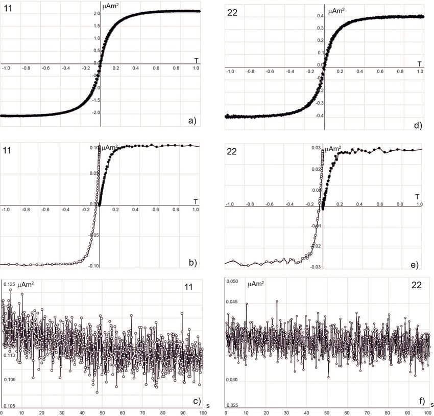
Appl. Sci. 2020, 10, 2073                                                                          4 of 15

2.4. Magnetic Analysis
     Dry lichen samples were placed in standard 8 cm3 palaeomagnetic plastic cubes for the analysis
of magnetic susceptibility and in pharmaceutical gel caps #4 for the hysteresis measurements. Mass
magnetic susceptibility (k) was calculated dividing the values measured with a KLY5 Agico meter
for the net weight of the samples. The coercive force (Bc), the saturation remanent magnetization
by mass (Mrs) and the saturation magnetization by mass (Ms) were measured using a vibrating
sample magnetometer (Micromag 3900, PMC) equipped with a carbon fibre probe, under cycling in a
maximum field of 1.0 T. Concentration dependent hysteresis parameters were calculated subtracting
the high field paramagnetic linear trend before dividing the magnetic moments for the net weight of the
samples. The coercivity of remanence (Bcr) values were extrapolated from backfield remagnetization
curves up to −1 T, following forward isothermal remanent magnetization up to a +1 T field.
     The percentage decay of Mrs after 100 s was calculated as:

                              Mrs (SP)% = 100 × (Mrs0 − MRs100 )/Mrs0 ,                               (1)

where SP refers to the superparamagnetic fraction, Mrs0 is the remanent magnetization measured as
soon as the magnetic field is reduced to noise levels after the application of a 1 T field, and Mrs100 is
the remanence measured 100 s later. The values of Mrs (SP)% are indicatory of the fraction of remanent
magnetization due to viscous magnetic components, which are usually carried by ultrafine magnetic
particles, dimensionally in the superparamagnetic/stable single domain boundary, which is around
20–35 nm for magnetite [16,17].
     The domain state and magnetic grain-size of the samples were compared to theoretical magnetite
according to the hysteresis ratios Mrs/Ms vs. Bcr/Bc in the “Day plot” [18–20].
     First order reversal curves (FORCs) [21,22] were measured using the Micromag operating software;
FORC diagrams were processed, smoothed and drawn with the FORCINEL Igor Pro routine [23].
FORCs were measured in steps of 2.5 mT, with 300 ms averaging time and maximum applied field
being 1.0 T. The optimum smoothing factor was evaluated by FORCINEL software.

2.5. Morphoscopic Observations
     Fragments from representative thalli were cut into pieces, mounted onto carbon stubs and then
coated with carbon in an Automatic Carbon Coater (Agar Scientific, Essex, UK). The sample surfaces
were observed under a Scanning Electron Microscopy (SEM Jeol JSM-5310) equipped with an INCA
Energy Dispersive Spectroscopy (EDS) system. Micrographs and spectra were collected with a 15 KV
operating voltage, 50–70 µA current, 20 mm work distance, and a 15–17 spot size (JSM-5310 data).
Micrographs were acquired by an INCA imagine capture system; spectra were collected by an INCA
X-stream pulse processor.

2.6. Statistical Analysis
      The magnitude of the relationship (effect size) between magnetic parameters and each
bioaccumulated element was evaluated by the coefficient of determination R2 , which estimates the
proportion of variance shared by the two variables, as explained by a linear model. As recommended
for environmental data [24], the probability of the effect size was estimated using the highest posterior
density intervals following a Bayesian approach [25]. In addition, Cohen’s ƒ2 was also calculated [26]
to class the effect size into small, medium and large [27]. Only R2 values at the lower point of the 95%
credible interval scored at least as medium size effect according to Cohen’s ƒ2 were retained. Prior to
analysis, data were transformed to logarithms to achieve normal distributions, and centered to zero
means in such a way that the intercept represents the value of the response variable at the mid-point of
the predictor range, and the original variance is retained. All calculations were done with the free
software R [28].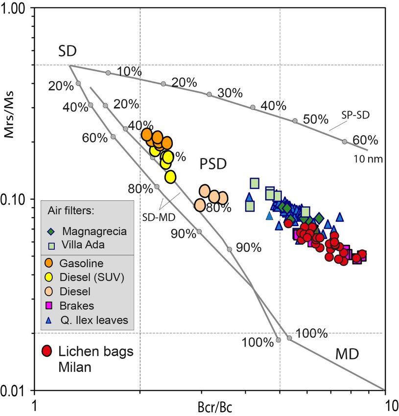
Appl. Sci. 2020, 10, 2073                                                                                  5 of 15

3. Results

3.1. Bioaccumulation of Trace Elements
     Lichen thalli transplanted at the control site showed values (Table 1) well within the range of
background concentrations for this species [29]. After 3 months of exposure in Milan, samples of
E. prunastri exhibited accumulation for all elements at all sites, with very few exceptions (Table 1),
with mean values exceeding those of the control sample by a factor 1.2 (Cd) to 6.3 (Sb). Differences in
concentrations across sites were in some cases remarkable, e.g., for Cu, which ranged between 6.5 and
55.4 µg/g dw.

      Table 1. Concentrations (µg/g dw) of trace elements in samples of the lichen Evernia prunastri exposed
      for 3 months at 25 sites in Milan, as well as at a control site (ctrl).

  Sample          Al        As        Cd          Cr         Cu         Fe         Pb          Sb         Zn
      1           422       0.28     0.072       3.7        11.4        841         4.4       0.49       42.8
      2           723       0.35     0.065       5.4        28.6       1269         5.6       0.95       36.8
      3           504       0.34     0.065       3.8        18.2        777         6.3       0.73       32.7
      4           279       0.25     0.059       2.3         6.5        471         4.1       0.55       33.8
      5           599       0.26     0.064       3.4        18.4        696         3.8       0.60       31.8
      6           428       0.31     0.074       6.9        55.4        932         5.8       0.83       36.8
      7           521       0.31     0.083       3.7        17.0        850         5.4       0.89       52.0
      8           882       0.37     0.066       4.2        14.6        959         4.4       0.72       32.6
      9           656       0.37     0.073       3.9        29.1        923         6.0       0.79       60.5
     10           509       0.28     0.070       2.9         8.9        631         4.1       0.51       27.1
     11           927       0.39     0.069       5.3        37.2       1253         4.6       1.38       46.7
     12           700       0.33     0.081       3.1        12.0        737         8.4       0.57       32.4
     13           657       0.31     0.080       3.0        11.2        720         3.4       0.41       17.1
     14           941       0.29     0.055       3.9        11.8        895         4.4       0.58       28.1
     15           639       0.32     0.077       3.3        13.8        790         5.1       0.77       34.0
     16           537       0.40     0.077       4.0        17.0        814         4.9       0.89       40.3
     17          1066       0.34     0.070       4.2        20.2       1061         6.6       0.96       44.4
     18           517       0.27     0.096       2.7         8.0        678         5.3       0.51       43.7
     19           449       0.30     0.058       2.8         6.6        666         3.9       0.56       28.3
     20           524       0.29     0.065       4.1        22.8        912         6.5       0.91       39.5
     21           459       0.30     0.065       3.2        17.8        740         8.2       0.81       50.0
     22           563       0.29     0.103       2.8         9.8        640        11.3       0.59       25.0
     23           569       0.32     0.077       4.2        24.4        901         8.3       0.83       42.1
     24           718       0.35     0.094       3.9        15.2        871        17.5       1.10       53.9
     25           616       0.30     0.088       3.0        16.0        719        16.4       1.01       37.2
    ctrl          429       0.21     0.061       1.7         3.3        442         2.0       0.12       27.1

3.2. Magnetic Measurements
     Magnetic susceptibility of E. prunastri transplants (Table 2) ranged between 7.8 and
35.8 × 10⁻⁸ m3 kg−1 , always exceeding 6–29 times the value of the control sample (1.2 × 10⁻⁸ m3 kg−1 )
(Figure 2).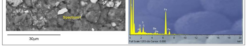
Appl. Sci. 2020, 10, 2073 6 of 15
Table 2. Magnetic parameters of samples of the lichen Evernia prunastri exposed for 3 months at 25 sites
in Milan, as well as at a control site (ctrl). k = mass magnetic susceptibility (10−8 m3 kg−1 ), Ms = mass
saturation magnetization (mAm2 kg−1 ), Mrs = mass saturation remanent magnetization (mAm2 kg−1 ),
Bc = coercivity (mT), Bcr = coercivity of remanence (mT), SIRM/k = saturation isothermal remanent
magnetization by magnetic susceptibility ratio (kA/m).
Sample k Ms Mrs Bc Bcr Bcr/Bc Mrs/Ms SIRM/k
1 13.31 9.06 0.52 5.84 37.20 6.37 0.06 3.93
2 26.10 25.16 1.66 7.06 40.88 5.79 0.07 6.35
3 12.49 8.51 0.53 6.01 38.74 6.44 0.06 4.23
4 8.77 7.32 0.45 5.53 35.83 6.48 0.06 5.19
5 16.38 19.41 0.94 4.88 40.71 8.35 0.05 5.72
6 20.32 20.57
Appl. Sci. 2020, 10, x FOR PEER REVIEW
1.45 6.89 40.75 5.92 0.07 6 of 17
7.14
7 13.72 10.04 0.63 5.59 40.33 7.21 0.06 4.63
8 17.07 8 20.68
17.07 1.16 1.16
20.68 5.41
5.41 39.09 39.09
7.23 7.23
0.06 0.06
6.82 6.82
9 13.21 9 9.07
13.21 0.56 0.56
9.07 5.86
5.86 37.55 37.55
6.41 6.41
0.06 0.06
4.24 4.24
10 8.78 10 7.58
8.78 0.53 0.53
7.58 6.18
6.18 38.45 38.45
6.23 6.23
0.07 0.07
6.07 6.07
11 35.8511 32.66
35.85 1.53 1.53
32.66 4.41
4.41 33.89 33.89
7.68 7.68
0.05 0.05
4.27 4.27
12 9.70 12 6.39
9.70 0.35 0.35
6.39 5.72
5.72 37.53 37.53
6.55 6.55
0.05 0.05
3.62 3.62
13 8.73 13 8.73
6.48 6.48
0.48 0.48 6.51
6.51 34.63 5.32
34.63 0.07
5.32 5.46
0.07 5.46
14 14.6314 14.63
7.31 7.31
0.44 0.44 6.15
6.15 35.72 5.81
35.72 0.06
5.81 3.01
0.06 3.01
15 14.6215 14.62
16.25 16.25
0.83 0.83 4.62
4.62 39.82 8.62
39.82 0.05
8.62 5.65
0.05 5.65
16 11.9816 11.98
12.54 12.54
0.70 0.70 5.27
5.27 38.95 7.39
38.95 0.06
7.39 5.83
0.06 5.83
17 22.93 17 22.93
15.81 15.81
0.82 0.82 4.86
4.86 37.23 7.67
37.23 0.05
7.67 3.57
0.05 3.57
18 10.0218 10.02
10.52 10.52
0.65 0.65 5.44
5.44 32.76 6.02
32.76 0.06
6.02 6.53
0.06 6.53
19 10.7119 10.71
8.33 8.33
0.40 0.40 4.67
4.67 34.69 7.42
34.69 0.05
7.42 3.74
0.05 3.74
20 26.02 20 26.02
23.71 23.71
1.36 1.36 5.38
5.38 37.73 7.01
37.73 0.06
7.01 5.22
0.06 5.22
21 17.17 8.44 0.42 5.03 35.08 6.97 0.05 2.43
21 17.17 8.44 0.42 5.03 35.08 6.97 0.05 2.43
22 7.75 22 7.75
5.95 5.95 0.39
0.39 6.22
6.22 36.69 5.90
36.69 0.07
5.90 4.99
0.07 4.99
23 27.11 20.97 1.14 5.50 38.65 7.03 0.05 4.21
23 27.11 20.97 1.14 5.50 38.65 7.03 0.05 4.21
24 15.53 13.22 0.94 6.26 37.36 5.96 0.07 6.03
24 15.53 13.22 0.94 6.26 37.36 5.96 0.07 6.03
25 9.22 9.31 0.55 5.26 37.88 7.20 0.06 5.96
25 9.22 9.31 0.55 5.26 37.88 7.20 0.06 5.96
ctrl 1.23 1.36 0.09 3.80 23.09 6.08 0.07 7.21
ctrl 1.23 1.36 0.09 3.80 23.09 6.08 0.07 7.21
Figure 2. Histograms of theofconcentration-dependent
Figure 2. Histograms magnetic
the concentration-dependent magnetic parameters,
parameters, normalized
normalized to the control
to the control
sample;
sample; black black columns
columns for magnetic
for magnetic susceptibility (k),
susceptibility (k), dithered
dithered forfor
Ms,Ms,
greygrey
for Mrs.
for Mrs.
All the hysteresis loops (Figure 3a, d) were similar in shape, narrow, saturated well before 1T,
All the hysteresis loops (Figure 3a,d) were similar in shape, narrow, saturated well before 1T,
with a modest variability of both coercivities [4.4 mT < Bc < 7.1 mT; 32.8 mT < Bcr < 40.9 mT] (Table
with a modest
2). Thevariability of both coercivities
concentration-dependent [4.4 mT <
magnetic parameters Bc <
(Table 2) 7.1 mT;less32.8
varied one
Appl. Sci. 2020, 10, 2073                                                                                            7 of 15

(Table 2). The concentration-dependent magnetic parameters (Table 2) varied less than one order of
magnitude [6.0 < Ms (mAm2 kg−1 ) < 32.7; 0.4 < Mrs (mAm2 kg−1 ) < 1.7] and, similarly to susceptibility
measurements, were 4–24 and 4–19 times in excess of the values of the control sample (Ms = 1.4
mAm2 kg−1 ; Mrs = 0.1 mAm2 kg−1 ) (Figure 2).
      Appl. Sci. 2020, 10, x FOR PEER REVIEW                                                                   7 of 17

            Figure 3. Hysteresis loops corrected for high-field linear trend (a,d), isothermal remanent
      Figure 3. Hysteresis loops corrected for high-field linear trend (a,d), isothermal remanent magnetization
            magnetization and backfield application (b,e) and Mrs decay in 100 s (c,f) for samples 11 and 22, the
      and backfield application (b,e) and Mrs decay in 100 s (c,f) for samples 11 and 22, the most and the
            most and the least intense of the dataset, respectively. Original data, not divided by mass.
      least intense of the dataset, respectively. Original data, not divided by mass.
            Overall, the hysteresis parameters indicated slightly variable concentrations of very similar soft
     Overall,     the hysteresis parameters indicated slightly variable concentrations of very similar
      ferrimagnetic minerals, presumably ascribable to magnetite. Consistently with susceptibility
soft ferrimagnetic
      measurements, minerals,
                        Ms and Mrspresumably        ascribable
                                     values were always     higher tothan
                                                                      magnetite.      Consistently
                                                                          in the control              with
                                                                                         sample. It was  notsusceptibility
                                                                                                              possible
measurements,
      to estimate Ms    and Mrs
                    the Curie      values were
                               temperature       always
                                             by means    of higher   than in the
                                                            magnetothermic         control
                                                                               curves,      sample.
                                                                                        given  the lowItsusceptibility
                                                                                                         was not possible
to estimate   the Curie
      values and           temperature
                    the noisy              by means
                              behaviour caused          of magnetothermic
                                                  by burning    of organic matter curves,
                                                                                     duringgiven   the low susceptibility
                                                                                            heating.
values and Mrsthe(SP)%
                   noisywas   estimatedcaused
                          behaviour      for samples   11 and of
                                                by burning      22 organic
                                                                    (Figure 3e,f),
                                                                             mattertheduring
                                                                                       most and   the least intense of
                                                                                               heating.
      the dataset,
     Mrs   (SP)% was respectively,
                         estimated and
                                     forshowed
                                          samplesthat
                                                    11the
                                                        andcontribution
                                                             22 (Figure of    rapidly
                                                                           3e,f),      decaying
                                                                                  the most   and components     to theof the
                                                                                                  the least intense
      overall  magnetization    is about  5%–6%.   This  result  is only indicative,  as errors
dataset, respectively, and showed that the contribution of rapidly decaying components to the    are large due  to the
                                                                                                                    overall
      relatively low values of magnetization and the short averaging time (100 ms).
magnetization is about 5%–6%. This result is only indicative, as errors are large due to the relatively
           The Mrs/Ms vs. Bcr/Bc ratios (Figure 4) indicated that the samples were distributed in the
low values of magnetization and the short averaging time (100 ms).
      middle-right side of the plot, between the theoretical curves calculated for mixtures of single domain
     The    Mrs/Ms vs. Bcr/Bc ratios (Figure 4) indicated that the samples were distributed in the
      (SD) and multidomain (MD) magnetite grains and that calculated for a mixture of SD and
middle-right    side of the plot,
      superparamagnetic            between the
                             (SP) magnetite     theoretical
                                             grains  [19,20]. curves calculated for mixtures of single domain (SD)
and multidomain (MD) magnetite grains and that calculated for a mixture of SD and superparamagnetic
(SP) magnetite grains [19,20].
Appl. Sci. 2020, 10, 2073                                                                                                                                 8 of 15

                              Appl. Sci. 2020, 10, x FOR PEER REVIEW                                                                  8 of 17

                                   Figure 4. Bilogarithmic Day plot of the hysteresis ratios Mrs/Ms vs. Bcr/Bc for transplanted lichens
      Figure 4. Bilogarithmic
                            EverniaDay      plot
                                    prunastri        of the
                                              (red dots)       hysteresis
                                                          compared  with Quercus ratios
                                                                                 ilex leavesMrs/Ms         vs.areas
                                                                                             from high traffic   Bcr/Bc
                                                                                                                    of Rome for
                                                                                                                            (greentransplanted lichens
                            triangles) [30], air filters from monitoring stations in Rome (green diamonds and squares) [31],
      Evernia prunastri (red      dots)      compared           with      Quercus         ilex  leaves       from      high    traffic areas of Rome
                            different kinds of fuel exhausts (orange, yellow and pink dots) and brake dusts (purple squares) [32].
      (green triangles) [30],Theair
                                  SD filters    from monitoring
                                      (single domain),     PSD (pseudo-singlestations
                                                                               domain) and  inMDRome       (greenfields
                                                                                                    (multidomain)      diamonds
                                                                                                                          and the    and squares) [31],
                            theorethical mixing trends for SD-MD and SP-SD pure magnetite particles (SP, superparamagnetic)
      different kinds of fuel   exhausts         (orange,       yellow      and
                            are taken from Dunlop [19,20]. Modified after [32].     pink     dots)    and      brake    dusts    (purple squares) [32].
      The SD (single domain),      PSD (pseudo-single domain) and MD (multidomain) fields and the theorethical
                            FORC diagrams (Figure 5) were made for two samples (11 and 20), selected for their relatively
      mixing trends forintense
                         SD-MD        andproperties;
                                magnetic      SP-SD the    pure   magnetite
                                                              distribution  peakedparticles
                                                                                       close to the(SP,
                                                                                                     originsuperparamagnetic)
                                                                                                             of the diagram and was     are taken from
                        dominated by viscous components of magnetization, typical for MD grains, without the
      Dunlop [19,20]. Modified         after    [32].
                        asymmetrical features which usually suggest the presence of SP ultrafine particles. The two FORC
                              diagrams are substantially identical, confirming that the samples contain variable concentrations of
     FORC diagrams  alike magnetic particles.
                       (Figure      5) were made for two samples (11 and 20), selected for their relatively
intense magnetic properties; the distribution peaked close to the origin of the diagram and was
dominated by viscous components of magnetization, typical for MD grains, without the asymmetrical
features which usually suggest the presence of SP ultrafine particles. The two FORC diagrams
are substantially identical, confirming that the samples contain variable concentrations of alike
magnetic particles.
              Appl. Sci. 2020, 10, x FOR PEER REVIEW                                                                                            9 of 17

                    Figure 5. FORC (First Order Reversal Curve) diagrams for samples 11 (a) and 20 (b); the smoothing
      Figure 5. FORC (First Order Reversal Curve) diagrams for samples 11 (a) and 20 (b); the smoothing
                factor was 5 and 4, respectively.
      factor was 5 and 4, respectively.
              3.3. Morphoscopic Observations
3.3. Morphoscopic Observations
                    Morphoscopic observations (Figure 6) clearly showed the accumulation of Fe-rich particles,
    Morphoscopic     observations
          ranging from                (Figure 6) clearly
                         clusters of submicrometric        showed
                                                      grains (Figurethe
                                                                     6a) accumulation     of Fe-rich
                                                                          to >10 μm, as well         particles,
                                                                                               as coarser and ranging
from clusters of submicrometric grains (Figure 6a) to >10 µm, as well as coarser and sometimes flaky
          sometimes  flaky metallic residuals (Figure 6b). Their chemical composition, as determined  by  EDS
              X-ray microanalysis, in addition to Fe, highlighted the widespread presence of elements such as Zn,
              Cu and Ba (Figure 6c). The shape and the recurrent inclusion of various elements other than Fe make
              these magnetic particles different from natural stoichiometric magnetite. Most morphologies were
              irregular, with rough and/or rounded and frictional surfaces, dissimilar to the spherical shapes of
              industrial fly ashes originated by the combustion of black and brown coal (e.g., [33–36]) or waste
              electrical and electronic equipment [37].
Appl. Sci. 2020, 10, 2073                                                                                     9 of 15

metallic residuals (Figure 6b). Their chemical composition, as determined by EDS X-ray microanalysis,
in addition to Fe, highlighted the widespread presence of elements such as Zn, Cu and Ba (Figure 6c).
The shape and the recurrent inclusion of various elements other than Fe make these magnetic particles
different from natural stoichiometric magnetite. Most morphologies were irregular, with rough and/or
rounded and frictional surfaces, dissimilar to the spherical shapes of industrial fly ashes originated by
the combustion       of black and brown coal (e.g., [33–36]) or waste electrical and electronic equipment
        Appl. Sci. 2020, 10, x FOR PEER REVIEW                                                    10 of 17
                                                                                                           [37].

      Figure 6. FESEM images and EDS spectra of selected particles embedded in the lichens exposed
             Figure 6. FESEM images and EDS spectra of selected particles embedded in the lichens exposed in
      in Milan;  (a) Spectrum 1; cluster of submicrometric Fe-rich particles; (b) coarse and flaky iron-rich
             Milan; (a) Spectrum 1; cluster of submicrometric Fe-rich particles; (b) coarse and flaky iron-rich
      residuals; (c) micrometric
             residuals;           particles,
                        (c) micrometric        rich
                                        particles,    ininFe,
                                                   rich    Fe,Cu
                                                               Cuand Ba.
                                                                 and Ba.

          3.4. Effect Size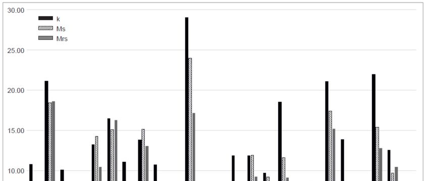
Appl. Sci. 2020, 10, 2073                                                                                     10 of 15

        Appl.Size
3.4. Effect   Sci. 2020, 10, x FOR PEER REVIEW                                                             11 of 17

    FigureFigure
             7 shows    the relationships
                    7 shows                 between
                             the relationships  betweenmagnetic
                                                         magneticsusceptibility     andelement
                                                                    susceptibility and    element  concentrations,
                                                                                                 concentrations,
      alongthe
along with   with  the credible
                 95%    95% credible  intervals
                                 intervals      (95CIs)
                                            (95CIs)     thetheR2Rvalues.
                                                     of of       2 values. The latter, along with the respective
                                                                           The latter, along with the respective
Cohen’s f 2 output,
      Cohen’s   ƒ2 output, are detailed
                      are detailed      in Table
                                    in Table  3. 3.

      Figure 7. Relationships between magnetic susceptibility and element concentrations, along with the
      95% credible
             Figure intervals  of the between
                     7. Relationships regression line. susceptibility and element concentrations, along with the
                                              magnetic
              95% credible intervals of the regression line.
     Only the correlations with Fe, Cr, Cu, and Sb showed a Cohen’s ƒ2 at least medium. In addition,
              R2 values
95CIs of theOnly   the correlations with
                           as well as Cohen’s       2 were
                                          Fe, Cr, ƒCu, and Sb showed aalso
                                                           calculated  Cohen’s   ƒ2 at least
                                                                           between           medium.
                                                                                        the four     In addition,
                                                                                                 chemical   elements
       95CIs  of the R 2 values as well as Cohen’s ƒ2 were calculated also between the four chemical elements
above (data not shown), showing strong intercorrelations among all elements, with Cohen’s ƒ2 always
       above (data
> medium.            not shown),
              Aluminium,          showing
                               which   is a strong
                                             majorintercorrelations
                                                      element in theamong  all elements,
                                                                      Earth’s  crust andwith hasCohen’s
                                                                                                 limitedƒ metabolic
                                                                                                         2 always

       > medium. Aluminium, which is a major element in the Earth’s crust and has limited metabolic
significance in lichens, is commonly used as a tracer of geogenic inputs, and correlations with this
       significance in lichens, is commonly used as a tracer of geogenic inputs, and correlations with this
element are roughly taken as an indication of soil contamination of samples [38]. 95CIs of R2 and
Cohen’s ƒ2 of Al with Fe, Cr, Cu and Sb (data not shown) highlighted only the correlation Al–Fe
Appl. Sci. 2020, 10, 2073 11 of 15
(R2 = 0.20–0.63, ƒ2 = 0.25 “medium”). Magnetic susceptibility was also very well correlated with the
other two concentration-dependent magnetic parameters Ms and Mrs (Table 3).
Table 3. Ninety-five percent credible intervals of the R2 values, Cohen’s ƒ2 and magnitude of the effect
size between magnetic susceptibility and chemical elements as well as other magnetic parameters.
R2 Cohen’s ƒ2 Effect Size
Al 0.00–0.36 0.00 small
As 0.00–0.36 0.00 small
Cd 0.00–0.30 0.00 small
Cr 0.43–0.73 0.75 large
Cu 0.36–0.70 0.56 large
Fe 0.51–0.76 1.04 large
Pb 0.00–0.14 0.00 small
Sb 0.23–0.64 0.30 medium
Zn 0.00–0.41 0.00 small
Ms 0.66–0.82 1.94 large
Mrs 0.51–0.76 1.04 large
4. Discussion
The results of bioaccumulation showed that Milan is quite homogeneously affected by high
deposition loads of elements such as Cr, Cu, Fe, and Sb; some more spotted peaks emerged also for Pb.
This outcome is consistent with other lichen biomonitoring studies in urban areas of Italy [37,39–42].
The results are indicative of a common origin of pollutants from non-exhaust sources of vehicular
traffic, such as brake abrasion. As a matter of fact, the above elements are used as components of brake
systems [43], and brake abrasion is reported as the main source of trace elements in PM [44].
This conclusion is supported by the results of EDS X-ray microanalysis, which pinpointed
the massive presence of Fe, and the widespread occurrence of Zn, Cu and Ba, the latter usually
being connected with emissions from car brakes and tyres [32,45]. In addition, as shown by SEM
analysis, Fe-rich particles are generally different from industrial spherical combustion particles, further
indicating that their source are motor vehicles and more specifically, relying on their composition,
break abrasion [32].
The range of the magnetic susceptibility values (7.8 to 35.8 × 10⁻⁸ m3 kg−1 ), when compared with
previous studies on transplanted lichens, is indicative of a notable concentration of magnetic minerals
and, consequently, of iron-rich bioaccumulated particles. Transplants of the lichen Pseudovernia
furfuracea exposed for 4 months in a complex and heavily polluted area, ranged from 7.1 to
17.1 × 10⁻⁸ m3 /kg−1 [37]. Transplants of the same lichen species exposed for 2 months in an industrial
area showed values in the range 0.4 to 7.4 × 10⁻⁸ m3 /kg−1 [46]. Transplants of Evernia prunastri exposed
for 6 months around a cement production plant in Slovakia showed magnetic susceptibility ranging
1.3 to 8.1 × 10⁻⁸ m3 /kg−1 [47]. Bags of Parmotrema pilosum exposed to atmospheric pollutants over the
course of 1 year increased from an initial mass-specific magnetic susceptibility value (mean ± S.D.) of
24.1 ± 5.0 × 10⁻⁸ m3 kg−1 to higher values up to 51.2 ± 23.0 × 10⁻⁸ m3 kg−1 [48]. This dataset included
three sites, two at metallurgical factories, and one influenced by vehicular emissions, where values
increased by 100%.
As emerged from the hysteresis loops, which are very similar and differ only for the
concentration-dependent magnetic parameters, which follow the same trend of magnetic susceptibility,
the variations of magnetic susceptibility are linked to different concentrations of magnetic particles
similar for composition and grainsize. The coercivities range, the low saturation field and the SIRM/k
values, spanning 2.4–7.1 kA/m, all suggest that magnetite-like minerals are the main magnetic carriers.
In the Day Plot, the lichens transplanted in Milan have been compared to the previous points
obtained for Quercus ilex leaves sampled in Rome, Italy, PM filters and dusts arising from fuel exhausts
and brakes’ emissions, as discussed in [32]. The transplants markedly overlap the “brake” samplesAppl. Sci. 2020, 10, 2073 12 of 15
and fall at the lower right end of the cluster defined by the particles accumulated on leaves and filters,
in a region of the plot falling in-between the theoretical trends for SD-MD and SD-SP pure magnetites,
far from “diesel” and “gasoline” exhausts, which instead follow the theoretical trends for mixtures of
single domain (SD) and multidomain (MD) magnetites. This result is at variance with the observations
of [37] for combustion dusts accumulated by lichens exposed in an area subjected to arsons, where the
magnetic mineralogy corresponded to magnetite-like minerals in PSD magnetic domain state/grain
size, similarly to the diesel exhaust emissions in [32].
Also the SIRM/k values (5.0 ± 1.2 kA/m) are compatible with the brake emissions (6.7 ± 2.5 kA/m)
and distinct from gasoline and diesel emissions (13.8 ± 6.3 kA/m and 14.5 ± 12.1 kA/m, respectively)
reviewed in [49]. Even FORC diagrams confirm the uniform prevalence, irrespective of the
concentration, of viscous components of magnetization, closely resembling the diagrams for brakes
and leaves reported by [32].
It is recalled that the critical magnetic grain size transitions, theoretically determined for
equidimensional magnetite, are about 0.03 µm for SP to SD, 0.08 µm for SD to PSD, and 17 µm
for PSD to true MD [50]. Overall, it is not easy to attribute these magnetic features to SP or MD particles.
In this sense, none of the magnetic properties diagnostic of the relevant presence of SP particles—
e.g., the enhancement of magnetic susceptibility, very low SIRM/k values, asymmetry along the Bu
axis in FORC diagrams—supported the presence of ultrafine magnetic particles, although the latter
could be linked to the choice of a relatively high averaging time (300 ms) during the measurements.
As a further difficulty, in traffic-related PM, the SP fraction may occur as coating of MD particles
and is originated by localized stress in the oxidized outer shell surrounding the unoxidized core of
magnetite-like grains; thus it cannot be considered as a direct proxy for the overall content of ultrafine
1 µm are
mostly generated. At higher operational temperatures (>190 ◦ C), the concentration of nanoparticles
(90% of total brake
dusts and constituting a major source of airborne magnetic nanoparticles. It is possible to speculate
that the coexistence of SP and MD particles is the result of both processes, and that SP particles,
for their intrinsically deciduous magnetic properties, are more difficult to be seen with standard room
temperature magnetic measurements.
As suggested by the relationship between Al and Fe, some proportion of these two metals may
also originate from soil resuspension. This is quite common, and in addition, it is known that, although
it is well known that brake wear constitutes one of the main sources of non-exhaust roadside PM,
brake wear accounts for 50%–60% of the total non-exhaust emissions [51].Appl. Sci. 2020, 10, 2073 13 of 15
5. Conclusions
From the present results, it is possible to conclude that magnetic properties of lichen transplants
are a robust proxy for the bioaccumulation of trace metals. The linear regression model with magnetic
susceptibility, as determined by the magnetic fraction of PM, explained large proportions of variance
for Fe, Cr, Cu, and Sb accumulated by E. prunastri. Chemical, magnetic and morphoscopic analysis
clearly pinpointed non-exhaust sources of vehicular traffic, notably brake abrasion, with a broad
grain-size range, as the main driver of PM air pollution in Milan.
The above relationships and the strong association of magnetic susceptibility with the
concentration-dependent hysteresis parameters suggest that magnetic susceptibility is a simple,
fast and very useful parameter that allows time- and cost-effective analysis of air pollution using
lichen transplants.
Author Contributions: S.L. and A.W. conceived and designed the experiments; T.C., A.V., S.S. and A.W. performed
the experiments; S.L. and A.W. analyzed the data; A.B. contributed analysis tools; S.L. and A.W. wrote the paper.
All authors have read and agreed to the published version of the manuscript.
Funding: Part of this research (magnetic analyses) was funded in the framework of FISR2016 project, promoted
by MIUR, the Italian Ministry of Education, University and Research.
Conflicts of Interest: The authors declare no conflict of interest. The funders had no role in the design of the
study; in the collection, analyses, or interpretation of data; in the writing of the manuscript, or in the decision to
publish the results.
References
1. WHO (World Health Organization). Available online: http://www.who.int/gho/phe/outdoor_air_pollution/
en/ (accessed on 18 March 2020).
2. Forsberg, B.; Hansson, H.C.; Johansson, C.; Areskoug, H.; Persson, K.; Jarvholm, B. Comparative health
impact assessment of local and regional particulate air pollutants in Scandinavia. Ambio 2005, 34, 11–19.
[CrossRef] [PubMed]
3. Karagulian, F.; Belis, C.A.; Dora, C.F.C.; Prüss-Ustün, A.M.; Bonjour, S.; Adair-Rohani, H.; Amann, M.
Contributions to cities’ ambient particulate matter (PM): A systematic review of local source contributions at
global level. Atmos. Environ. 2015, 120, 475–483. [CrossRef]
4. Loppi, S. Lichens as sentinels for air pollution at remote alpine areas (Italy). Environ. Sci. Pollut. Res. 2014,
21, 2563–2571. [CrossRef] [PubMed]
5. Loppi, S.; Paoli, L. Comparison of the trace element content in transplants of the lichen Evernia prunastri
and in bulk atmospheric deposition: A case study from a low polluted environment (C Italy). Biologia 2015,
70, 460–466. [CrossRef]
6. Loppi, S.; Frati, L.; Paoli, L.; Bigagli, V.; Rossetti, C.; Bruscoli, C.; Corsini, A. Biodiversity of epiphytic lichens
and heavy metal contents of Flavoparmelia caperata thalli as indicators of temporal variations of air pollution
in the town of Montecatini Terme (central Italy). Sci. Total Environ. 2004, 326, 113–122.
7. Loppi, S. May the diversity of epiphytic lichens be used in environmental forensics? Diversity 2019, 11, 36.
[CrossRef]
8. Contardo, T.; Giordani, P.; Paoli, L.; Vannini, A.; Loppi, S. May lichen biomonitoring of air pollution be used
for environmental justice assessment? A case study from an area of N Italy with a municipal solid waste
incinerator. Environ. Forensics 2018, 19, 265–276. [CrossRef]
9. Loppi, S.; Ravera, S.; Paoli, L. Coping with uncertainty in the assessment of atmospheric pollution with
lichen transplants. Environ. Forensics 2019, 20, 228–233. [CrossRef]
10. Maher, B.A.; Ahmed, I.A.M.; Karloukovski, V.; MacLaren, D.A.; Foulds, P.G.; Allsop, D.; Mann, D.M.A.;
Torres-Jardòn, R.; Calderon-Garciduenas, L. Magnetite pollution nanoparticles in the human brain. Proc. Natl.
Acad. Sci. USA 2016, 113, 10797–10801. [CrossRef]
11. Calderón-Garcidueñas, L.; González-maciel, A.; Mukherjee, P.S.; Reynoso-Robles, R.; Pérez-Guillé, B.;
Gayosso-Chávez, C.; Torres-Jardón, R.; Cross, J.V.; Ahmed, I.A.M.; Karloukovski, V.V.; et al. Combustion-
and friction derived magnetic air pollution nanoparticles in human hearts. Environ Res. 2019, 176. [CrossRef]Appl. Sci. 2020, 10, 2073 14 of 15
12. Hofman, J.; Maher, B.A.; Muxworthy, A.R.; Wuyts, K.; Castanheiro, A.; Samson, R. Biomagnetic monitoring
of atmospheric pollution: A review of magnetic signatures from biological sensors. Environ. Sci. Technol.
2017, 51, 6648–6664. [CrossRef] [PubMed]
13. Loppi, S.; Pacioni, G.; Olivieri, N.; Di Giacomo, F. Accumulation of trace metals in the lichen Evernia prunastri
transplanted at biomonitoring sites in central Italy. Bryologist 1998, 101, 451–454. [CrossRef]
14. Paoli, L.; Fačkovcová, Z.; Guttová, A.; Maccelli, C.; Kresáňová, K.; Loppi, S. Evernia goes to school:
Bioaccumulation of heavy metals and photosynthetic performance in lichen transplants exposed indoors
and outdoors in public and private environments. Plants 2019, 8, 125. [CrossRef] [PubMed]
15. Vannini, A.; Paoli, L.; Nicolardi, V.; Di Lella, L.A.; Loppi, S. Seasonal variations in intracellular trace element
content and physiological parameters in the lichen Evernia prunastri transplanted to an urban environment.
Acta Bot. Croat. 2017, 76, 171–176. [CrossRef]
16. Sagnotti, L.; Winkler, A. On the magnetic characterization and quantification of the superparamagnetic
fraction of traffic-related urban airborne PM in Rome, Italy. Atmos. Environ. 2012, 59, 131–140. [CrossRef]
17. Wang, X.; Løvlie, R.; Zhao, X.; Yang, Z.; Jiang, F.; Wang, S. Quantifying ultrafine pedogenic magnetic particles
in Chinese loess by monitoring viscous decay of superparamagnetism. Geochem. Geophys. Geosyst. 2010, 11,
10. [CrossRef]
18. Day, R.; Fuller, M.; Schmidt, V.A. Hysteresis properties of titanomagnetites: Grain-size and compositional
dependence. Phys. Earth Planet. Inter. 1977, 13, 260–267. [CrossRef]
19. Dunlop, D.J. Theory and application of the Day plot (MRS/MS versus HCR/HC) 1. Theoretical curves and
tests using titanomagnetite data. J. Geophys. Res. 2002, 107. [CrossRef]
20. Dunlop, D.J. Theory and application of the Day plot (MRS/MS versus HCR/HC) 2. Application to data for
rocks, sediments, and soils. J. Geophys. Res. 2002, 107. [CrossRef]
21. Pike, C.R.; Roberts, A.P.; Verosub, K.L. Characterizing interactions in fine magnetic particle systems using
first order reversal curves. J. Appl. Phys. 1999, 85, 6660–6667. [CrossRef]
22. Roberts, A.; Pike, C.R.; Verosub, K.L. First-order reversal curve diagrams: A new tool for characterizing the
magnetic properties of natural samples. J. Geophys. Res. 2000, 105, 28461–28475. [CrossRef]
23. Harrison, R.J.; Feinberg, J.M. FORCinel: An improved algorithm for calculating first-order reversal curve
distributions using locally weighted regression smoothing. Geochem. Geophys. Geosyst. 2008, 9. [CrossRef]
24. Feckler, A.; Low, M.; Zubrod, J.P.; Bundschuh, M. When significance becomes insignificant: Effect sizes
and their uncertainties in Bayesian and frequentist frameworks as an alternative approach when analyzing
ecotoxicological data. Environ. Toxicol. Chem. 2018, 37, 1949–1955. [CrossRef] [PubMed]
25. Gelman, A.; Goodrich, B.; Gabry, J.; Vehtari, A. R-squared for Bayesian regression models. Am. Stat. 2019, 73,
307–309. [CrossRef]
26. Selya, A.S.; Rose, J.S.; Dierker, L.C.; Hedeker, D.; Mermelstein, R.J. A practical guide to calculating Cohen’s
f2, a measure of local effect size, from proc mixed. Front. Psychol. 2012, 3, 111. [CrossRef] [PubMed]
27. Cohen, J.E. Statistical Power Analysis for the Behavioral Sciences; Lawrence Erlbaum Associates, Inc.: Hillsdale,
NJ, USA, 1988.
28. R Core Team. R: A Language and Environment for Statistical Computing; R Foundation for Statistical Computing:
Vienna, Austria, 2020; Available online: https://www.R-project.org/ (accessed on 18 March 2020).
29. Cecconi, E.; Fortuna, L.; Benesperi, R.; Bianchi, E.; Brunialti, G.; Contardo, T.; Di Nuzzo, L.; Frati, L.;
Monaci, F.; Munzi, S.; et al. New interpretative scales for lichen bioaccumulation data: The Italian proposal.
Atmosphere 2019, 10, 136. [CrossRef]
30. Szönyi, M.; Sagnotti, L.; Hirt, A.M. On leaf magnetic homogeneity in particulate matter biomonitoring
studies. Geophys. Res. Lett. 2007, 34, L06306. [CrossRef]
31. Sagnotti, L.; Macrì, P.; Egli, R.; Mondino, M. Magnetic properties of atmospheric particulate matter from
automatic air sampler stations in Latium (Italy): Toward a definition of magnetic fingerprints for natural and
anthropogenic PM10 sources. J. Geophys. Res. 2006, 111, B12. [CrossRef]
32. Sagnotti, L.; Taddeucci, J.; Winkler, A.; Cavallo, A. Compositional, morphological, and hysteresis
characterization of magnetic airborne particulate matter in Rome, Italy. Geochem. Geophys. Geosyst.
2009, 10. [CrossRef]
33. Sarbak, Z.; Stanczyk, A.; Kramer-Wachowiak, M. Characterization of surface properties of various fly ashes.
Powder Technol. 2004, 145, 82–87. [CrossRef]Appl. Sci. 2020, 10, 2073 15 of 15
34. Veneva, L.; Hoffmann, V.; Jordanova, D.; Jordanova, N.; Fehr, T. Rock magnetic, mineralogical and
micro-structural characterization of fly ashes from Bulgarian power plants and the nearby anthropogenic
soils. Phys. Chem. Earth 2004, 29, 1011–1023. [CrossRef]
35. Jordanova, D.; Hoffmann, V.; Fehr, K.T. Mineral magnetic characterization of anthropogenic magnetic phases
in the Danube river sediments (Bulgarian parts). Earth Planet. Sci. Lett. 2004, 221, 71–89. [CrossRef]
36. Jordanova, D.; Jordanova, N.; Hoffmann, V. Magnetic mineralogy and grain-size dependence of hysteresis
parameters of single spherules from industrial waste products. Phys. Earth Planet. Inter. 2006, 154, 255–265.
[CrossRef]
37. Winkler, A.; Caricchi, C.; Guidotti, M.; Owczarek, M.; Macrì, P.; Nazzari, M.; Amoroso, A.; Di Giosa, A.;
Listrani, S. Combined magnetic, chemical and morphoscopic analyses on lichens from a complex anthropic
context in Rome, Italy. Sci. Total Environ. 2019, 690, 1355–1368. [CrossRef]
38. Loppi, S.; Pirintsos, S.A.; De Dominicis, V. Soil contribution to the elemental composition of epiphytic lichens
(Tuscany, central Italy). Environ. Monit. Assess. 1999, 58, 121–131. [CrossRef]
39. Giordano, S.; Adamo, P.; Sorbo, S.; Vingiani, S. Atmospheric trace metal pollution in the Naples urban area
based on results from moss and lichen bags. Environ. Pollut. 2005, 136, 431–442. [CrossRef]
40. Loppi, S.; Corsini, A.; Paoli, L. Estimating environmental contamination and element deposition at an urban
area of central Italy. Urban Sci. 2019, 3, 76. [CrossRef]
41. Paoli, L.; Munzi, S.; Fiorini, E.; Gaggi, C.; Loppi, S. Influence of angular exposure and proximity to vehicular
traffic on the diversity of epiphytic lichens and the bioaccumulation of traffic-related elements. Environ. Sci.
Pollut. Res. 2013, 20, 250–259. [CrossRef]
42. Vannini, A.; Paoli, L.; Russo, A.; Loppi, S. Contribution of submicronic (PM1 ) and coarse (PM > 1) particulate
matter deposition to the heavy metal load of lichens transplanted along a busy road. Chemosphere 2019, 231,
121–125. [CrossRef]
43. Bonfanti, A. Low-Impact Friction Materials for Brake Pads. Ph.D. Thesis, University of Trento, Trento, Italy,
June 2016.
44. Thorpe, A.; Harrison, R. Sources and properties of non-exhaust particulate matter from road traffic: A review.
Sci. Total Environ. 2008, 400, 270–282. [CrossRef]
45. Sanders, P.G.; Xu, N.; Dalka, T.M.; Maricq, M.M. Airborne brake wear debris: Size distributions, composition,
and a comparison of dynamometer and vehicle tests. Environ. Sci. Technol. 2003, 37, 4060–4069. [CrossRef]
[PubMed]
46. Kodnik, D.; Candotto Carniel, F.; Licen, S.; Tolloi, A.; Barbieri, P.; Tretiach, M. Seasonal variations of PAHs
content and distribution patterns in a mixed land use area: A case study in NE Italy with the transplanted
lichen Pseudevernia furfuracea. Atmos. Environ. 2015, 113, 255–263. [CrossRef]
47. Paoli, L.; Winkler, A.; Guttová, A.; Sagnotti, A.; Grassi, A.; Lackovičová, A.; Senko, D.; Loppi, S. Magnetic
properties and element concentrations in lichens exposed to airborne pollutants released during cement
production. Environ. Sci. Pollut. Res. 2017, 24, 12063–12080. [CrossRef] [PubMed]
48. Marié, D.C.; Chaparro, M.A.E.; Sinito, A.M. Magnetic biomonitoring of airborne particles using lichen
transplants over controlled exposure periods. SN Appl. Sci. 2020, 2, 104. [CrossRef]
49. Gonet, T.; Maher, B.A. Airborne, vehicle-derived Fe-bearing nanoparticles in the urban environment—A
review. Environ. Sci. Technol. 2019, 53, 9970–9991. [CrossRef]
50. Butler, R.F.; Banerjee, S.K. Theoretical single-domain grain size range in magnetite and titanomagnetite.
J. Geophys. Res. 1975, 80, 4049–4058. [CrossRef]
51. Harrison, R.M.; Jones, A.M.; Gietl, J.; Yin, J.; Green, D.C. Estimation of the contributions of brake dust, tire
wear, and resuspension to nonexhaust traffic particles derived from atmospheric measurements. Environ.
Sci. Technol. 2012, 46, 6523–6529. [CrossRef]
© 2020 by the authors. Licensee MDPI, Basel, Switzerland. This article is an open access
article distributed under the terms and conditions of the Creative Commons Attribution
(CC BY) license (http://creativecommons.org/licenses/by/4.0/).You can also read