Meta-Analysis of Generalized Additive Models in Neuroimaging Studies
←
→
Page content transcription
If your browser does not render page correctly, please read the page content below
Meta-Analysis of Generalized Additive Models in
                                                           Neuroimaging Studies

                                            Øystein Sørensena,∗, Andreas M Brandmaierd,e , Didac Maciá Brosc , Klaus
                                            Ebmeierf , Paolo Ghislettag,h,i , Rogier A Kievitj , Athanasia M Mowinckela ,
                                                  Kristine B Walhovda,b , Rene Westerhausena , Anders Fjella,b
arXiv:2002.02627v1 [stat.AP] 7 Feb 2020

                                              a Center    for Lifespan Changes in Brain and Cognition, University of Oslo, Norway
                                              b Department     of Radiology and Nuclear Medicine, Oslo University Hospital, Norway
                                            c Departament de Medicina, Facultat de Medicina i Ciències de la Salut, Universitat de

                                                     Barcelona, and Institut de Neurociències, Universitat de Barcelona, Spain
                                           d Center for Lifespan Psychology, Max Planck Institute for Human Development, Berlin,

                                                                                       Germany
                                             e Max Planck UCL Centre for Computational Psychiatry and Ageing Research, Berlin,

                                                                                       Germany
                                                                 f Department of Psychiatry, University of Oxford, UK
                                               g Faculty of Psychology and Educational Sciences, University of Geneva, Switzerland
                                                                    h Swiss Distance University Institute, Switzerland
                                                 i Swiss National Centre of Competence in Research LIVES, University of Geneva,

                                                                                      Switzerland
                                                      j MRC Cognition and Brain Sciences Unit, University of Cambridge, UK

                                          Abstract
                                          Analyzing data from multiple neuroimaging studies has great potential in terms
                                          of increasing statistical power, enabling detection of effects of smaller magnitude
                                          than would be possible when analyzing each study separately and also allowing
                                          to systematically investigate between-study differences. Restrictions due to pri-
                                          vacy or proprietary data as well as more practical concerns can make it hard to
                                          share neuroimaging datasets, such that analyzing all data in a common location
                                          might be impractical or impossible. Meta-analytic methods provide a way to
                                          overcome this issue, by combining aggregated quantities like model parameters
                                          or risk ratios. Most meta-analytic tools focus on parametric statistical models,
                                          and methods for meta-analyzing semi-parametric models like generalized ad-
                                          ditive models have not been well developed. Parametric models are often not
                                          appropriate in neuroimaging, where for instance age-brain relationships may
                                          take forms that are difficult to accurately describe using such models. In this
                                          paper we introduce meta-GAM, a method for meta-analysis of generalized ad-
                                          ditive models which does not require individual participant data, and hence is
                                          suitable for increasing statistical power while upholding privacy and other regu-
                                          latory concerns. We extend previous works by enabling the analysis of multiple

                                             ∗ Corresponding author: Øystein Sørensen, Department of Psychology, Pb. 1094 Blindern,

                                          0317 Oslo, Norway.
                                               Email address: oystein.sorensen@psykologi.uio.no (Øystein Sørensen)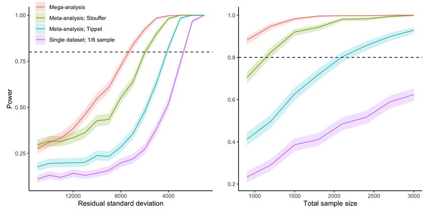
model terms as well as multivariate smooth functions. In addition, we show
how meta-analytic p-values can be computed for smooth terms. The proposed
methods are shown to perform well in simulation experiments, and are demon-
strated in a real data analysis on hippocampal volume and self-reported sleep
quality data from the Lifebrain consortium. We argue that application of meta-
GAM is especially beneficial in lifespan neuroscience and imaging genetics. The
methods are implemented in an accompanying R package metagam, which is also
demonstrated.
Keywords: data protection, distributed learning, generalized additive mixed
models, generalized additive models, meta-analysis, privacy

1. Introduction
    Combining brain imaging data across studies has great potential in terms
of increasing statistical power, enabling discoveries of effects that might not
be detectable in any single dataset. Due to regulatory and practical concerns,
privacy in particular, it may not be possible to analyze all data in a single place.
It may also sometimes be beneficial to analyze data from multiple studies in two
stages, even when the data are available at a single location, e.g., when data do
not fit in computer memory or runtime is nonlinear in the number of participants
(Riley et al., 2010).
    Meta-analytic techniques offer one way to increase statistical power without
sharing raw data. By estimating the relationships under study separately in
each data location, pooled estimates are obtained by combining the estimates
without sharing the underlying data. With some exceptions, meta-analytic
methods have been developed for combining parameters from parametric statis-
tical models or for effect measures like relative risks (Hedges and Olkin, 1985;
Sutton and Higgins, 2008). However, there are important cases in which it is
impractical and suboptimal to enforce a parametric representation of the as-
sociation under investigation, e.g., when an appropriate parametric model to
approximate the data is not known, or its interpretability is not clear, as with
high-degree polynomials (Wood, 2017). Examples include lifetime trajectories
of brain development (Fjell et al., 2010), air quality measures (Gasparrini and
Armstrong, 2010), and ecological phenomena (Borchers et al., 1997; Pedersen
et al., 2019). Generalized additive models (GAMs) (Hastie and Tibshirani, 1986;
Wood, 2017) are attractive for studying such relationships, and can easily be
extended to longitudinal or other forms of clustered data via generalized addi-
tive mixed models (GAMMs), which, in addition to GAMs, can also estimate
random effects.
    Figure 1 illustrates modeling lifespan trajectories of hippocampal volume
changes using linear mixed models (LMMs) with quadratic and cubic polyno-
mials for the age term, and a GAMM with a smooth term for age. The LMMs
were fitted using R (R Core Team, 2019) package nlme (Pinheiro et al., 2019)
and the GAMM was fitted using mgcv (Wood, 2017), all with a random in-
tercept term. The data were taken from 4,364 observations of 2,023 healthy

                                         2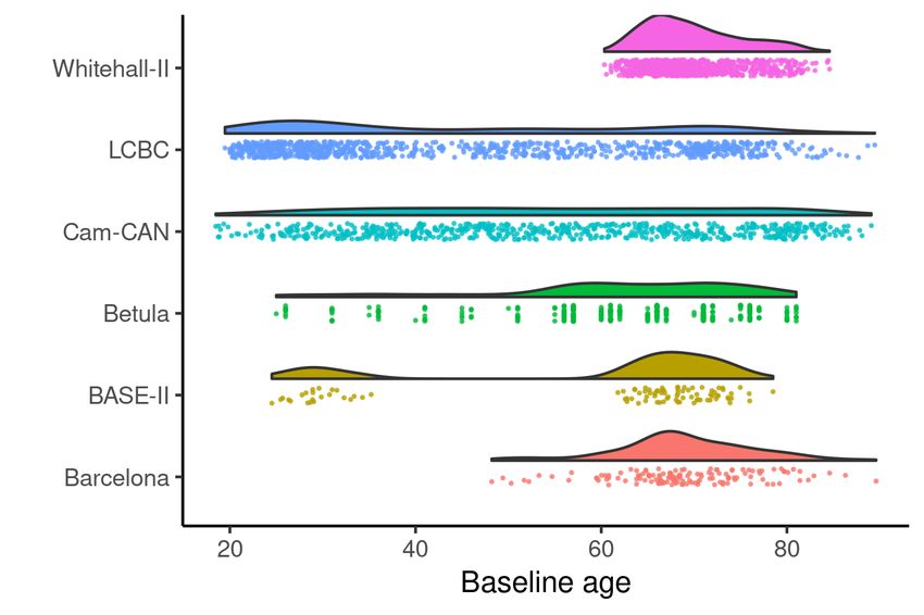
Figure 1: Modeling lifespan trajectories. Example of modeling lifespan hippocampal
volume with longitudinal data using linear mixed models with quadratic and cubic terms for
age, as well as a generalized additive model. The black dots show individual observations and
the black lines connect subsequent observations from the same individual. The GAMM was
fitted with 20 cubic regression splines and a random intercept term for each individual, and
the optimal smoothing parameter estimated with restricted maximum likelihood.

participants (age 4-93 years, 1-8 measurements per participant) from the Cen-
ter for Lifespan Changes in Brain and Cognition longitudinal studies (Walhovd
et al., 2016; Fjell et al., 2017). Detailed sample characteristics are presented in
the Supplementary Material. The quadratic fit is not flexible enough to capture
the steep increase during adolescence - moreover, it estimates the hippocampal
volume to increase until the age of around 40. The cubic fit captures the volume
growth during adolescence better than the quadratic fit, but fails to capture the
decline that occurs after the age of around 70. The GAMM fit, on the other
hand, is flexible enough to both capture the steep increase during adolescence,
a period of moderate decline during adulthood, and finally a steeper decline
at older age. All figures in this paper were created using ggplot2 (Wickham,
2016).
    As the methods for meta-analysis of GAMs and GAMMs are identical, we
will refer to both as GAMs in the rest of this paper, unless distinction is neces-
sary. For reasons that we will explain below, in this paper we will not discuss
meta-analysis of the underlying parametric functions across GAMs. Rather, we
present methods for combining GAM fits for neuroimaging data by pointwise
meta-analysis of the fitted values. Although developed for use in meta-analytic
neuroimaging studies, the methods can of course be applied to other types of
data as well. The models under study can include any number of terms, includ-
ing multivariate smooth functions. In order to employ these techniques, models
should be fit independently in each cohort, with basis functions and knot place-
ment optimal to their given dataset. We hence extend the previous work by

                                             3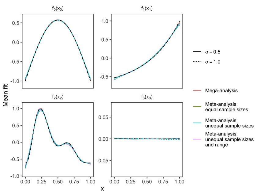
Schwartz and Zanobetti (2000) who combined univariate fits from Gaussian ad-
ditive models. Sauerbrei and Royston (2011) also proposed a somewhat related
approach using fractional polynomials, although requiring individual partici-
pant data being available. The methods developed by Sauerbrei and Royston
(2011) have also been used by Crippa et al. (2018) who compared strategies
for dose-reponse meta-analysis for computing relative risk estimates using both
fractional polynomials and cubic spline models.
    The main application we have in mind is multi-center studies in which it is
impractical or not possible to analyze all brain imaging data in a single loca-
tion. This is for instance the case for the Enhancing Neuro Imaging Genetics
Through Meta Analysis project (ENIGMA: http://enigma.ini.usc.edu/), where
meta-analysis of individual site summary statistics is the commonly applied
strategy (e.g., Dennis et al. (2018); van Erp et al. (2018)). The methods de-
veloped require that some model relating an outcome of interest to a set of
explanatory variables has been fitted on data from each cohort, and that the
model estimates can be shared across cohorts such that the expected response
and their standard errors at new values of the explanatory variables can be com-
puted. We provide a companion R package named metagam (Sørensen et al.,
2020) containing functions for removing all individual participant data from
GAMs fitted with the mgcv and gamm4 packages (Wood, 2017; Wood and Scheipl,
2017), such that the resulting model object only contains aggregate measures
which can easily be shared. The package also contains methods for combining
the fits and analyzing the results, and will be demonstrated in Section 5. The
comprehensive review of meta-analysis packages in R by Polanin et al. (2017)
does not mention any existing packages for conducting this type of pointwise
meta-analysis, so to the best of our knowledge, metagam is the first R package
to provide this functionality.
    The methods presented in this paper were motivated by a project in the
Lifebrain consortium (http://www.lifebrain.uio.no/) (Walhovd et al., 2018). The
goal was to study the relationship between self-reported sleep and hippocampal
volume across six Lifebrain cohorts, and GAMMs were a natural model choice
due to the expected non-linear age-relationships for self-reported sleep param-
eters and hippocampal volume. In this case a safe common data store was in
place, but we initially hypothesized that it might be easier to have each cohort
fit a model locally and share the overall result rather than analyzing all data in
a single place, leading to the development of the methods presented here.

2. Background

2.1. Meta-Analysis
    Consider a situation in which M cohorts m = 1, . . . , M each have a dataset
Dm with nm observations of a response y and p explanatory variables rep-
resented by a vector x with p elements. In the cross-sectional case, there is
one observation per study participant, so the data for each cohort can be rep-
resented by Dm = {(yi , xi1 , . . . , xip ) = (yi , xi ), for i = 1, . . . , nm }. In the

                                           4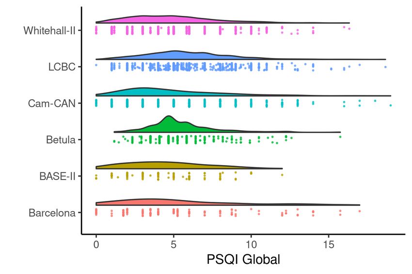
longitudinal case, we assume subject i in cohort m has been measured nmi
times. Notably, this includes the case of individually varying numbers of assess-
ments and time intervals betweens assessments. The data are now represented
by Dm = {(yij , xij1 , . . . , xijp ) = (yij , xij ), for i = 1, . . . , nm , j = 1, . . . , nmi }.
In practice, some of the explanatory variables will be time-varying, while others
will be time-invariant.
    Our interest concerns performing statistical inference on data from all co-
horts, in the case where data cannot be shared across cohorts and analyzed
jointly. When the relationship under study can be represented by a paramet-
ric model, well established methods exist for obtaining meta-analytic estimates
of the model parameters. For example, if the data are cross-sectional and a
generalized linear model (McCullagh and Nelder, 1989)

                                       g(µ) = η = x0 β,                                        (1)

is being used, where g(·) is some link function and µ = E(y) is the expected
response, estimates β̂ m from each cohort can be combined using either fixed
or mixed effect meta-analysis (DerSimonian and Laird, 1986; Gasparrini et al.,
2012). The covariance matrix V (β̂ m ) of β̂ m is used to define meta-analytic
weights and to compute standard errors of the combined estimates. Linear
regression is a special case of (1) with identity link g(µ) = µ and observed
responses deviating from the mean according to a normal distribution with
standard deviation σ: y ∼ N (µ, σ 2 ).
    An extension of (1) to longitudinal data is straightforward, by using linear
mixed models (Laird and Ware, 1982) of the form

                                   g(µ) = η = x0 β + z0 b,

where b represents the subject-specific random effects and z is the explanatory
variable vector for the random effects. The fixed effect estimates β̂ m would be
combined in exactly the same way as for linear models.
    There is a variety of similar and related approaches in other modeling frame-
works, such as structural equation modeling to model individual differences in
change over time (e.g., Brandmaier et al. (2018); Kievit et al. (2018)) but they
all share the property that they are parametric models that are grounded in
some a priori theory about the change process under investigation.

2.2. Generalized Additive Models
    In many applications, assuming that a linear predictor η is a smooth function
of the explanatory variables, rather than following the model (1) that is linear
in its parameters (e.g., polynomial), may lead to better statistical fit, cf. Figure
1. Generalized additive models (GAMs) (Hastie and Tibshirani, 1986) take this
approach. For example, with a univariate smooth term for each explanatory
variable, the model becomes

                         g(µ) = η = β0 + f1 (x1 ) + · · · + fp (xp ),                          (2)

                                                5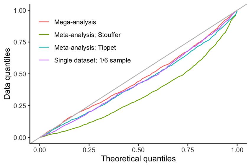
where each function fj (xj ) is assumed to be smooth in xj . Another example is
a model with a single bivariate smooth term (Wood, 2006),

                            g(µ) = η = β0 + f1 (x1 , x2 ).                         (3)

In general, we let Xs denote the set of explanatory variables used by smooth
function fs (·). Hence, in (2), Xs = {xs } for s = 1, . . . , p, and in (3), Xs =
{x1 , x2 } for s = 1. We can thus write a GAM with S smooth terms on the form
                                                 S
                                                 X
                           g(µ) = η = β0 +             fs (Xs ) ,                  (4)
                                                 s=1

where β0 denotes the intercept. As each smooth term is only uniquely deter-
mined up to some additive constant, some constraints have to be imposed in
the fitting procedure. Details are discussed in Appendix A.
   Each smooth function fs is typically defined as a linear combination of Ks
basis functions bk (·) with weights γk , k = 1, . . . , Ks ,
                                           Ks
                                           X
                              fs (Xs ) =         bk (Xs )γk .                      (5)
                                           k=1

A linear term for xj can be obtained by setting Xs = {xj } and fs (Xs ) = βs xj .
Common basis functions include cubic regression splines, P-splines, and thin
plate regression splines (TPRS) (Wood, 2017).
    Figure 2 illustrates how a smooth function is constructed from four cubic
regression splines using (5). The left panel shows the splines b1 (x), . . . , b4 (x),
and the colored dots indicate the knot location of the respective spline. The
colored curves in the right panel shows the contribution from each spline to the
sum in (5) when using weights (γ1 , γ2 , γ3 , γ4 ) = (1, 0.2, −0.2, 0.5), and the black
curve shows the resulting smooth function fs (x).

2.3. Smoothing
    With the exception of TPRS, the basis functions commonly used are char-
acterized by knots placed along each covariate axis. In the case of TPRS, the
basis functions are instead low rank approximations of thin plate splines. Sim-
ply fitting a model of the form (2) using least squares or maximum likelihood
with a large number of basis functions for each smooth typically leads to overly
wiggly fits. Hence, model selection or smoothing methods are required. One
approach is to fit models with a successively decreasing number of knots, and
comparing them using some model selection criterion, e.g., AIC (Hastie et al.,
2009, Sec. 5.2.2). However, when fitting models with more than one smooth
term, and possibly with multivariate terms, the number of possible combina-
tions of knots becomes impractically high. An attractive alternative is to make
sure the number of knots is set high enough to capture the nonlinearity of the

                                           6
Figure 2: Constructing a smooth function from splines. The left panel shows four cubic
regression splines, with knot locations indicated by the colored dots. The right panel shows
the contribution from each spline when using weights (γ1 , γ2 , γ3 , γ4 ) = (1, 0.2, −0.2, 0.5), and
the black curve shows the resulting smooth function fs (x).
association being modeled, and then add a wiggliness penalty. With the com-
mon second derivative penalty, the criterion to be minimized in the Gaussian
case with identity link function is
n
( S
)2 S Z
2
X X X
yi − β0 − fs (Xs,i ) + λs {fs00 (Xs )} dXs , (6)
i=1 s=1 s=1
where λs is the smoothing parameter for the sth term. An optimal value of
λ = (λ1 , . . . , λs )0 can be obtained using, e.g., generalized cross-validation, re-
stricted maximum likelihood, or marginal maximum likelihood. This smoothing
approach is used, e.g., by the R package mgcv (Wood, 2017).
Figure 3 shows the impact of the smoothing parameter λ on the lifespan hip-
pocampal volume curves from Figure 1. The fits were computed using 50 cubic
regression splines with knots equally spaced over the range of age values in the
data. Using restricted maximum likelihood, the optimal smoothing parameter λ
was estimated to 434. The black line represents this optimal value, which appro-
priately captures the nonlinearities without being too wiggly. The gray curves
show a range of fits with λ between 1 and 107 . The curves with low smoothing
follow the same overall trend as the optimal curve, but are quite wiggly, par-
ticularly during late adolescence and early adulthood. On the other hand, the
curves with high λ are smooth, but do not capture the actual nonlinearity in
the data.
2.4. Knot Placement
If each cohort used exactly the same basis functions, including knot place-
ment, all basis function weights could in principle be combined by treating the
7Figure 3: Smoothing parameter controls wiggliness. Impact of the smoothing parameter
λ on the lifespan trajectories of hippocampal volume from Figure 1. The black line shows the
fit corresponding to λ = 434, which is optimal in terms of maximizing the restricted maximum
likelihood. The gray lines show a range of fits with λ between 1 and 107 . The annotations
show the function estimates in each extreme end of the range of smoothing parameters, as
well as the optimal estimate.
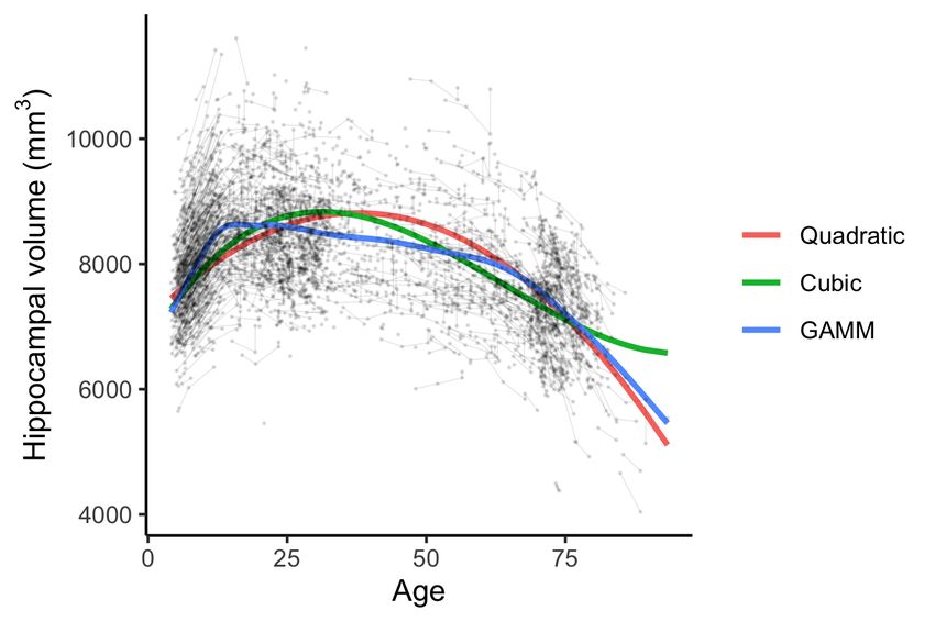
Figure 4: Eigenvalues are sensitive to range of explanatory variables. Eigenvalue
spectrum of the cross-product matrix over 100 random simulations using knot locations as
shown in the left plot, with x uniformly distributed over range shown in legend. Error bars
show the sample standard deviations.
8weights as linear regression parameters, as shown by Gasparrini et al. (2012). In
practice, this approach is most often not feasible, as the best fitting GAMs will
have varying basis function bk (·). As also noted by Crippa et al. (2018), if the
range of some explanatory variable xj differs between cohorts, e.g. the age-range
used in the study, the knot placement may be suboptimal at best or even lead to
non-identified models. As an example, we sampled a variable x uniformly over
ranges [0, 1], [0.25, 1] and [0.5, 1], computed a linear predictor matrix X using
seven cubic regression splines, and then computed the eigenvalue spectrum of
the cross-product matrix X 0 X. Zero eigenvalues of the cross-product matrix
indicates that the spline basis is not of full rank. Figure 4 shows the average
eigenvalue spectrum over 100 random simulations. In the case x ∈ [0, 1] none of
the eigenvalues were zero, and a model would be identified. However, when x
was distributed over [0.25, 1], one eigenvalue was on average very close to zero
and when the range was [0.5, 1], three eigenvalues were very close to zero. The
practical consequence of zero eigenvalues is that some model coefficients, basis
function weights in this case, would not be identified. Although imposing ad-
ditional penalization like the ridge (Hoerl and Kennard, 1970) may identify a
solution while also shrinking the parameters towards zero, a better solution is
to let the range of each separate dataset determine its knot locations.
As a concrete example of this identifiability problem, we consider modeling of
lifespan trajectories of hippocampal volumes from six European cohorts. The
data are further described in Section 5. As shown in Figure 10 (top), these
cohorts have widely varying age distributions. We fit GAMs relating baseline age
to hippocampal volume in each cohort, but enforced the same knot location for
the models in each cohort. Knots were placed at eight equally spaced quantiles
of the full data sample. Table 1 shows the corresponding spline coefficients,
cf. eq. (5). A parametric meta-analysis using the methods of Gasparrini et al.
(2012) would combine each of these parameters in order to create a meta-analytic
fit. However, as can be seen, cohorts Barcelona and Whitehall-II have missing
values (NA) for spline coefficient γ2 due to nonidentifiability. In addition, there
are extreme outliers: Barcelona has a severely outlying value for γ1 , BASE-II
has an outlying value for γ8 , and Whitehall-II has outlying values for γ1 and
γ3 . This lack of identification and unstable coefficients is caused by using knot
locations which, because they are forced to be equal across the cohorts, are far
from the actual age distributions in these cohorts.
3. Pointwise Meta-Analysis of Generalized Additive Models
We now propose a model for meta-analysis of GAMs. We start by assuming
that a GAM has been fitted on the data from each cohort separately, obtaining
estimates
S
X
g(µ̂m ) = η̂m = fˆm (x) = β̂0,m + fˆs,m (Xs ) , m = 1, . . . , M (7)
s=1
of the relationships under study, where the subscript m denotes cohort. Each
model term has a corresponding estimated standard deviation σ̂s,m (Xs ), and
9Cohort γ1 γ2 γ3 γ4 γ5 γ6 γ7 γ8
Barcelona 28142 - 6195 7719 7629 7421 7190 6310
BASE-II 4694 8374 6274 7919 7770 7213 7297 -17182
Betula 9605 8481 8380 8072 7840 7389 6994 7734
Cam-CAN 8298 8452 8397 8040 7916 7468 7291 6375
LCBC 8408 8479 8324 7689 7401 7468 7202 5819
Whitehall-II 1625151 - -120033 7580 7528 7353 6935 6084
Table 1: Spline coefficients for models described in Section 2.4. The coefficient γ2 was not pos-
sible to determine for Barcelona and Whitehall-II. In addition, γ1 for Barcelona and Whitehall-
II, γ3 for Whitehall-II, and γ8 for BASE-II are severe outliers.
the overall fit has estimated standard deviation σ̂m (x). Importantly, x rep-
resent some grid of values of explanatory variables over which a meta-analytic
estimate of the regression function is sought, and Xs is the corresponding subset
of variables for smooth term s. Equation (7) computes the expected response
over this grid for cohort m.
We illustrate our methods by considering meta-analytic estimation of each
single term separately, but note that inference on any combination of smooth
terms, including the overall function, is readily obtained with the same methods.
Some additional details related to identification of smooth terms are discussed
in Appendix A. For ease of notation, we omit the dependency on Xs in the rest
of this section. For example, fs,m means fs,m (Xs ) and σs,m means σs,m (Xs ).
In the fixed effects meta-analysis case, the overall fit is computed as the
weighted mean
PM ˆ −2
ˆ m=1 fs,m σ̂s,m
fs = P M −2
. (8)
m=1 σ̂s,m
with standard error ( )−1/2
M
X
−2
sefˆs = σ̂s,m . (9)
m=1
In the random effects case, the between-study variance σs2 is first estimated
pointwise. The estimator
PM −2 ˆ
m=1 σ̂m,s fs − (M − 1)
σ̂s = max 0, P . (10)
M −2 P M −4 PM −2
m=1 σ̂m,s − m=1 σ̂m,s / m=1 σ̂m,s
was introduced by DerSimonian and Laird (1986) and used by, e.g., Sauerbrei
and Royston (2011). As opposed to, e.g., restricted maximum likelihood esti-
mation, (10) may appear computationally attractive since it does not require
iteration. However, as shown by Veroniki et al. (2016), iterative methods may
give more accurate estimates. Next, the overall fit is computed using
2 −1
PM ˆ 2
ˆ m=1 fs,m σ̂s,m + σ̂s
fs = PM (11)
2 −1
2
m=1 σ̂s,m + σ̂s
10with standard error
( M
)−1/2
X
2
sefˆs = σ̂s,m + σ̂s2 . (12)
m=1
Formulas (8)-(12) are the familiar weighted means formulas used in meta-
analysis, and have been used by Sauerbrei and Royston (2011) in a similar set-
ting, focusing on meta-analysis of univariate functions estimated by fractional
polynomials. In the fixed effects case, fˆs is the estimated mean conditional on
randomly pooling from the populations of the observed cohorts alone. Random
effects analysis, on the other hand, estimates the marginal population effect fs
across all potential studies. See Viechtbauer (2010, Sec. 2.3) for an excellent
discussion of the interpretation of fixed vs. random effects meta-analyses. Con-
fidence bands with level (1 − α) are readily obtained for either estimates as
h i
fˆs + zα/2 sefˆs , fˆs + z1−α/2 sefˆs , (13)
where zq denotes the qth quantile of the standard normal distribution.
Tests for statistical significance of smooth terms can be performed by com-
bining the p-values from each separate fit using methods for meta-analytic com-
bination of p-values as summarized, e.g., in Becker (1994). In particular, let ps,m
denote the p-value obtained in cohort m for the hypothesis H0,m : fs (Xs ) = 0
that the smooth term s is zero over the whole range of explanatory variables Xs
in cohort m, and let HA,m : fs (Xs ) 6= 0 denote the alternative hypothesis. Such
p-values can be computed using the methods in Wood (2012). The meta-analytic
null hypothesis then states that all p-values are uniformly distributed between 0
and 1, i.e., H0 : ps,m ∼ U (0, 1), m = 1, . . . , M , while the meta-analytic alterna-
tive hypothesis HA states that all p-values have the same unknown non-uniform
density which is non-increasing in the test statistic (Birnbaum, 1954). A large
number of methods exist for computing the combined p-values. For example,
Stouffer’s sum of z method (Stouffer et al., 1949) uses the Z-score
PM
wm Φ−1 (1 − ps,m )
Zs = m=1qP , (14)
M 2
m=1 m w
where Φ is the standard normal distribution and Φ−1 its quantile function, and
wm , m = 1, . . . , M are meta-analytic weights. Zaykin (2011) suggests defining
√
the weights as the square root of the sample size, wm = nm . The combined
p-value is then defined by ps = 1 − Φ(Zs ).
In order to compute either fixed effect estimates using (8) and (9) or random
effect estimates using (11) and (12), we require the availability of some method
for computing predictions and standard errors for each model term. In the GAM
case, this requires knowledge of the basis functions and corresponding weights
estimated in each study, as well as their covariance matrix. These quantities
are readily available from software for fitting GAMs, like mgcv (Wood, 2017)
or pyGAM (Servn and Brummitt, 2018). Importantly, the individual participant
11Figure 5: Functions used in simulations. True functional forms used in simulations in
Section 4.1.
data are not required for any of these procedures, and the basis functions need
not be equal across cohorts.
4. Simulation Studies
4.1. Function Estimation
In order to investigate the statistical performance of the meta-analytic ap-
proach presented in the previous section, we conducted a simulation study in
which data were generated from the model
y = f0 (x0 ) + f1 (x1 ) + f2 (x2 ) + f3 (x3 ) + .
All explanatory variables were independently uniformly distributed in [0, 1] and
∼ N (0, σ 2 ). The functional forms assumed were similar to those used by
Marra and Wood (2012), and shown in Figure 5.
Datasets with 4,000 observations of (x0 , x1 , x2 , x3 , y) were independently
sampled 1,000 times. Each set of simulations was run with residual standard
deviation σ = 0.5 and σ = 1. For each dataset, the following three cases were
considered:
• In the mega-analysis case, all 4,000 observations were analyzed jointly.
This served as a gold standard, yielding the model that would be fit if all
data were available to analyze with a single model.
12• In the equal sample size case, the dataset was split into 5 ”cohorts” of
800 observations each. Each cohort was analyzed independently, and the
meta-analytic fit computed as outlined above.
• In the unequal sample size case, the dataset was split into 5 ”cohorts”
with 300, 500, 800, 1,000, and 1,400 observations each.
• In the unequal range and sample size case, a first ”cohort” was created by
sampling 300 observations with x2 < 0.5 from the full dataset, the second
cohort by sampling 500 observations with x2 ≥ 0.5 from the remaining
observations, the third cohort by sampling 800 observations with x1 < 0.5
from the remaining observations, the fourth cohort by sampling 1,000
observations with x1 ≥ 0.5 from the remaining observations, and the fifth
cohort contained the remaining 1,400 observations. Hence, this case has
the same sample sizes as the unequal sample size case, but the ranges of
x1 and x2 vary between cohorts.
In the latter three cases, fixed effects meta-analysis was conducted. In all
cases, univariate smooth terms were estimated using cubic regression splines
with 20, 10, 30, and 5 basis functions for f0 (x0 ), f1 (x1 ), f2 (x2 ), and f3 (x3 ), re-
spectively. Second derivative smoothing was performed using generalized cross-
validation, and standard error computations for each term included the uncer-
tainty about the overall intercept as described in Marra and Wood (2012). The
smooth terms were subject to a point constraint at the midpoint x0 = x1 =
x2 = x3 = 0.5 to ensure that the terms were identified and comparable across
cohorts, cf. Appendix A. Both the meta-analytic fits and the mega-analytic
fit were shifted along the y-axis to ensure that they summed to zero over [0, 1],
making them comparable to the true functional forms. All computations were
performed in R version 3.6.2 (R Core Team, 2019) with the package mgcv (Wood,
2017).
Figure 6 shows the average fits over all simulations. One can hypothesize
that splitting a dataset into smaller parts and performing smoothing separately
might lead to oversmoothing compared to analyzing all data in a single model.
Considering Figure 6 we see that this is the case for estimating f2 (x2 ) in the
case with σ = 1, in which all meta-analysis cases slightly underestimated the
two peaks of the true term. In the case of σ = 0.5, however, all meta-analysis
estimated had very low bias. The two meta-analyses with unequal sample size,
also had somewhat too smooth estimates of f1 (x1 ) in the σ = 1 case. Overall,
however, the average fits in the meta-analysis cases were very close to the true
curves.
Table 2 shows the root-mean-square error (RMSE) of the fitted terms over
the range [0, 1]. In both noise settings, the meta-analyses with equal and unequal
sample size had only slightly higher RMSE than the mega-analytic estimates,
and there did not seem to be any systematic difference between them. The
meta-analysis with unequal range and sample size had somewhat higher RMSE
for f1 (x1 ) and f2 (x2 ), corresponding to the two variables whose range differed
13Figure 6: Simulation estimates overlaid on true functions. Dashed black lines show
true functions. The colored lines show mean fits averaged over 1,000 simulations as described
in Section 4.1.
14Equal sample Unequal sample Unequal range
Term σ Mega-analysis
size size and sample size
f0 (x0 ) 0.50 0.022 (0.005) 0.022 (0.005) 0.021 (0.005) 0.020 (0.006)
f1 (x1 ) 0.50 0.019 (0.006) 0.019 (0.006) 0.027 (0.010) 0.017 (0.005)
f2 (x2 ) 0.50 0.035 (0.006) 0.035 (0.006) 0.037 (0.009) 0.030 (0.005)
f3 (x3 ) 0.50 0.008 (0.005) 0.008 (0.005) 0.008 (0.005) 0.009 (0.006)
f0 (x0 ) 1.00 0.036 (0.011) 0.036 (0.011) 0.036 (0.011) 0.035 (0.013)
f1 (x1 ) 1.00 0.036 (0.014) 0.036 (0.013) 0.045 (0.016) 0.031 (0.012)
f2 (x2 ) 1.00 0.061 (0.011) 0.061 (0.011) 0.070 (0.019) 0.054 (0.011)
f3 (x3 ) 1.00 0.017 (0.010) 0.017 (0.010) 0.018 (0.010) 0.018 (0.013)
Table 2: Mean root-mean-square error of fitted terms in the case of equal sample sizes, unequal
sample sizes, and mega-analysis, with residual standard deviation σ = 0.5 or σ = 1. Standard
deviations across simulations are shown in parentheses.
Equal sample Unequal sample Unequal range
Term σ Mega-analysis
size size and sample size
f0 (x0 ) 0.50 0.94 (0.24) 0.94 (0.24) 0.94 (0.24) 0.96 (0.20)
f1 (x1 ) 0.50 0.94 (0.25) 0.94 (0.24) 0.82 (0.39) 0.97 (0.17)
f2 (x2 ) 0.50 0.89 (0.31) 0.90 (0.30) 0.87 (0.34) 0.96 (0.20)
f3 (x3 ) 0.50 0.99 (0.10) 0.99 (0.11) 0.99 (0.10) 0.99 (0.12)
f0 (x0 ) 1.00 0.96 (0.20) 0.96 (0.19) 0.96 (0.19) 0.98 (0.16)
f1 (x1 ) 1.00 0.91 (0.29) 0.91 (0.28) 0.83 (0.38) 0.97 (0.17)
f2 (x2 ) 1.00 0.88 (0.33) 0.88 (0.32) 0.82 (0.39) 0.96 (0.21)
f3 (x3 ) 1.00 0.99 (0.12) 0.99 (0.12) 0.98 (0.13) 0.98 (0.13)
Table 3: Mean coverage of 95 % confidence intervals for fitted terms in the case of equal sample
sizes, unequal sample sizes, and mega-analysis, with residual standard deviation σ = 0.5 or
σ = 1. Standard deviations across simulations are shown in parentheses.
between cohorts. For the terms f0 (x0 ) and f3 (x3 ), the unequal range and sample
size case had RMSE very close to the two other meta-analytic cases.
Table 3 shows the average coverage across [0, 1] of 95 % confidence intervals
computed with (13). The coverage of the confidence intervals of the mega-
analytic estimates were close to 95 %, as expected from Marra and Wood (2012),
and always conservative. For the meta-analysis with equal and unequal sample
size, the coverage varied between 88 % and 99 %. In particular for f1 (x1 ) and
f2 (x2 ) the confidence intervals were somewhat too narrow for these scenarios.
The unequal range and sample size case had poorer coverage for f1 (x1 ) and
f2 (x2 ), varying between 82 % and 87 %. For f0 (x0 ) and f3 (x3 ), on the other
hand, all three meta-analytic cases had very similar coverage.
4.2. Hypothesis Testing and Power
As mentioned in Section 3, p-values for smooth terms combined in a meta-
analytic fit can be computed using methods for meta-analysis of p-values. Two
issues are of particular interest in this regard; first, whether their distribution is
close to uniform when the null hypothesis is true, and second, the power to reject
15Figure 7: Lifespan trajectories with group interaction. Functional forms assumed for
lifespan trajectories in Section 4.2. Subjects are assumed to belong to either group 0 or 1,
whose mean lifespan trajectories differ as shown by the two curves.
a false null hypothesis. Simulation experiments were conducted to investigate
both issues. A nonlinear functional form was assumed as shown in Figure 7, rep-
resenting the lifespan trajectory of the volume of a brain region of interest. For
the power analysis, it was assumed that a dichotomous group variable interacted
with the lifespan trajectory, leading to slightly higher atrophy for members of
the baseline group, especially in advanced ages. For analysis of the null dis-
tribution of p-values, the two groups had identical lifespan trajectories. The
shapes of the functional forms were taken from an estimate of lifespan trajec-
tory of cerebellum cortex volume using data from Center for Lifespan Changes
in Brain and Cognition longitudinal studies (Walhovd et al., 2016; Fjell et al.,
2017). Analyzing this type of smooth interactions is relevant, e.g., when inves-
tigating the impact of a given genetic variation on lifespan trajectories of brain
measures (Walhovd et al., 2019).
Our goal was to compare the p-value distribution under the null hypothesis
and the power to detect an interaction between the smooth function and group
membership for a mega-analysis and for the meta-analysis approach developed
in this paper. Cross-sectional measurements were simulated with age uniformly
distributed between 4 and 94 years, and group memberships randomly allocated
to 0 or 1 with equal probabilities. For the mega-analysis, all measurements were
analyzed in a single GAM, while for the meta-analysis, the data were first split
into 6 datasets and analyzed separately, before a meta-analytic p-value was
computed. For reference, the power obtained when using a single dataset of size
1/6th of the total dataset was also computed. A total of 1,000 Monte Carlo
samples were analyzed for each parameter setting. For the case of a nonzero
group interaction, statistical power was computed as the fraction of the 1,000
16random simulations in which the group interaction was significant at a 5 %
level. In the first set of simulations, the total sample size was fixed at 3,000
while the residual standard deviation varied between 1,000 and 15,000. In the
second set of simulations, the residual standard deviation was fixed at 3,500,
and the total sample size varied between 900 and 3,000. In all cases, ”cohort
fits” were computed by randomly splitting the dataset into 6 equally sized parts.
The GAM used to analyze the data was of the form
y = β0 x0 + f1 (x1 ) + f2 (x1 ) x0 + ,
where x0 ∈ {0, 1} is an indicator for group membership and x1 is age, and is
a normally distributed residual. The parameter β0 represents the offset effect
of group membership, the smooth term f (x1 ) represents the age trajectory of
subjects in group 0, and f2 (x1 ) represents the difference between the smooth
term of subjects in group 1 and subjects in group 0. Hence, subjects in group
1 have age trajectory given by f1 (x1 ) + f2 (x1 ). GAMs were fitted with the
gam function in mgcv (Wood, 2017), using cubic regression splines to construct
the smooth terms and generalized cross-validation for smoothing. The null hy-
pothesis states that there is no difference between the lifespan trajectories across
groups, i.e., the p-values were calculated for H0 : f2 (x1 ) = 0 in the mega-analysis
and separately for H0,m : f2 (x1 ) = 0, m = 1, . . . , 6 in the meta-analysis. For
the mega-analysis, the p-values were directly available from the model object
returned by mgcv, which uses the methods described in Wood (2012). For the
meta-analysis, we compared several different methods for combining p-values:
Wilkinson’s maximum p (Wilkinson, 1951), Tippet’s minimum p (Tippet, 1931),
the logit-p method (Becker, 1994), Fisher’s sum of logs (Fisher, 1925), Edging-
ton’s sum of p (Edgington, 1972), and Stouffer’s sum of z (Stouffer et al., 1949),
using the implementations in the R package metap (Dewey, 2019). See Loughin
(2004) for an in-depth comparison of methods for combining p-values. As all
samples in the meta-analysis were of equal size, equal meta-analytic weights
were used in Stouffer’s sum of z (14). The other methods do not use weights.
Tippet’s minimum p method gave p-values closest to a uniform under the null
hypopothesis under most parameter settings, while Stouffer’s sum of z method
typically gave highest power. The p-values resulting from these two methods are
hence shown in the results in this section, while complete results for all methods
can be found in the Supplementary Material.
Figure 8 shows quantile-quantile plots of the p-values obtained by meta-
analysis, mega-analysis, and a fit of a single dataset in the case of no actual
interaction between the group variable and the lifespan trajectories in the case
with sample size 3,000 and residual standard deviation 3,500. Results for other
values of these parameters were similar, and are shown in the Supplementary
Material. The gray line shows the ideal reference line. All methods yielded
p-values which deviated to some degree from the uniform distribution. Meta-
analytic p-values computed using Tippet’s minimum p method were close to the
p-values obtained either in the mega-analysis or in the single data fit. p-values
computed using Stouffer’s sum of z, on the other hand, were considerably further
from being uniformly distributed. The lack of uniformity for the p-values of the
17Figure 8: P-value distribution under the null hypothesis. Quantile-quantile plot of p-
values under the null hypothesis as described in Section 4.2, for the case of residual standard
deviation equal to 3,500 and total sample size 3,000. Meta-analytic p-values were computed
using both Stouffer’s and Tippet’s method, as shown by the legend.
mega-analysis can be explained by the approximate nature of the algorithm
used to compute them, due to the need take into account the uncertainty of the
smoothing parameter λ, cf. Wood (2017, Sec. 6.12).
Figure 9 (left) shows power curves over a range of noise values, and Figure
9 (right) shows power curves over a range of sample sizes. In both cases, the
mega-analytic approach outperforms the meta-analytic approaches. Stouffer’s
sum of z method obtained power closest to the mega-analysis, while Tippet’s
minimum p method had lower power. As expected, analyzing a single dataset,
representing 1/6th of the total data, gave much lower power than either of the
other two approaches.
To summarize, meta-analysis using Stouffer’s sum of z method had power
fairly close to that of a mega-analysis, at an increased risk of falsely rejecting
true null hypotheses. On the other hand, meta-analysis using Tippet’s min-
imum p method had risk of falsely rejecting a true null hypothesis close to
that of a mega-analysis, at the cost of lower power. The other methods for
combining p-values were somewhere inbetween these extremes, as shown in the
Supplementary Material.
5. Case Study
We will now illustrate the proposed methods on brain imaging data from six
European cohorts analyzed by Fjell et al. (2019), using the R package metagam
which implements the methods described in this paper. The datasets contained
measurements of sleep quality and hippocampal volume from the Berlin Study
18Figure 9: Statistical power to detect interaction. Results of statistical power simulations
desribed in Section 4.2. Left: fixed total sample size 3,000 and varying noise level. Right:
fixed noise level σ=3,500 and varying total sample size. Shaded areas around curves show 95
% confidence intervals computed using the R package Hmisc (Harrell Jr et al., 2019). Meta-
analytic p-values were computed using both Stouffer’s and Tippet’s method, as shown by the
legend.
of Aging-II (BASE-II) (Bertram et al., 2013; Gerstorf et al., 2016), the Betula
project (Nilsson et al., 1997), the Cambridge Centre for Ageing and Neuro-
science study (Cam-CAN) (Taylor et al., 2017), Center for Lifespan Changes in
Brain and Cognition longitudinal (LCBC) studies (Walhovd et al., 2016; Fjell
et al., 2017), Whitehall-II (Filippini et al., 2014), and University of Barcelona
brain studies (Abellaneda-Pérez et al., 2019; Rajaram et al., 2017; Vidal-Piñeiro
et al., 2014). Self-reported sleep and hippocampal volume data from 2,843 par-
ticipants (18-90 years) were included. Longitudinal information on hippocampal
volume was available for 1,065 participants, yielding a total of 4,621 observa-
tions. Mean interval from first to last examination was 3.8 years (range 0.2-11.0
years). Participants were screened to be cognitively healthy and in general not
suffer from conditions known to affect brain function, such as dementia, major
stroke, multiple sclerosis, etc. Exact screening criteria were not identical across
subsamples. Detailed sample characteristics are presented in the Supplementary
Material.
In Fjell et al. (2019), the data were analyzed jointly using GAMMs in a
mega-analysis, taking into account both the clustering of repeated measure-
ments within the same subject, and of subjects within a given cohort. However,
the methods proposed in this paper enable this type of multi-cohort analysis
also when the data cannot be shared. In this particular example we examine
how hippocampal volume is related to age and to sleep quality as measured by
the global score on the Pittsburgh Sleep Quality Index (PSQI) (Buysse et al.,
1989). A low value of the PSQI variable indicates good sleep.
19The following model was first fit to data from each cohort separately:
yij = β0 + f1 (xij,1 ) + f2 (xij,1 )xi,2 + β3 xi,3 + bi + ij . (15)
yij denotes hippocampal volume of subject i at timepoint j, xij,1 is the age of
subject i at timepoint j, xi,2 is the global PSQI score, and xi,3 is the sex of
subject i. bi ∼ N (0, σb2 ) is the random intercept of subject i and ij ∼ N (0, σ 2 )
is the residual. The main effect of age is represented by f1 (x1 ). f2 (x1 )x2
is a varying-coefficient term (Hastie and Tibshirani, 1993), in which f2 (x1 ) is
a regression coefficient for sleep quality which varies smoothly with age. The
model fits were computed using the gamm function in mgcv (Wood, 2017), except
for the data from Whitehall-II, which did not contain repeated measurements
and were computed using gam. Restricted maximum likelihood was used for
both for estimating the smoothing parameter and estimation of random effect
terms, and cubic regression splines were used as basis functions. The range of
the age variable differed considerably between cohorts, as shown in the top part
of Figure 10. Hence, both the knot placement and the number of knots used
to fit f1 (x1 ) and f2 (x1 ) was determined for each cohort separately. The knots
were placed within the range of x1 in each cohort. Using the second derivative
penalty (6), the smoothing is determined by λ rather than by the number of
knots, as long as the number of knots is sufficiently high to allow for a wide range
of functional forms; this was tested using the simulation procedure described in
Wood (2017, Ch. 5.9). The sleep quality scores were similarly distributed across
cohorts, as shown in the bottom part of Figure 10. Betula differs somewhat in
shape from the others, due to a transformation that had to be applied to these
data (Fjell et al., 2019).
Except for additional arguments to s specifying the type of basis function
and the number of knots, the following code was used to fit the model for
each cohort. The argument pc = 70 defines a point constraint f2 (70) = 0
for the varying-coefficient term, ensuring that the estimates of this term are
comparable across cohorts, as described in Appendix A. Details are shown in
the Supplementary Material.
library(mgcv)
# Fit GAMM in cohort 1
cohort_gam1Figure 10: Empirical distribution of explanatory variables. Raincloud plots (Allen
et al., 2019; Whitaker et al., 2019) showing the distribution of baseline age (top) and global
PSQI score (bottom) in the data from each cohort studied in Section 5.
21Figure 11: Age trajectories for each cohort. Estimates of β0 + f1 (x1 ) in (15), showing how age predicts hippocampal volume in each cohort. Gray shaded areas are 95 % confidence intervals. without any individual data. The following lines attach the metagam package and then creates an object cohort_fit1, which does not contain any individual- specific data. library(metagam) cohort_fit1
# Create a grid over which to compute meta-analytic fits
grid
Figure 12: Comparison of meta-analytic and mega-analytic estimates. Meta-analytic
fits obtained as described in Section 5, compared to the corresponding fit obtained with full
data. Left: effect of age on hippocampal volume, including the overall intercept. Right:
Interaction effect of age and PSQI global score on hippocampal volume.

13 (left) for the main effect of age on hippocampal volume. The plot shows that
LCBC and Cam-CAN are the main contributors to the meta-analytic fit for
ages up to around 50 years, after which the relative influence of the other studies
starts increasing. Furthermore, the heterogeneity of the models fit in each study
can be analyzed by computing Cochran’s Q statistic (Cochran, 1954) over an
explanatory variable, thus comparing fˆs,m for m = 1, . . . , M independently at
each value of the explanatory variable. Figure 13 (right) shows a heterogeneity
plot comparing the main effects of age in each study, with 95 % confidence
intervals represented by the shaded gray areas. From age 60 and above, there
seems to be evidence of heterogeneity among the contributing studies. Using
metagam, such plots are obtained with the command:

plot_dominance(metafit_age)
plot_heterogeneity(metafit_age)

   We refer to the online package documentation for more examples on how to
use metagam to compute meta-analytic fits.

6. Discussion

    We have proposed and illustrated a flexible way to obtain meta-analytic fits
of generalized additive mixed models in neuroimaging studies where individual
participant data cannot be shared across cohorts. In the simulation studies, the
meta-analytic procedure showed estimation performance close to that obtained
in the ideal case, in which all data were analyzed in a single model, except that

                                             24
Figure 13: Dominance and heterogeneity plots. Dominance and heterogeneity plots for
β0 + f1 (x1 ) in equation (15). Left: the relative contribution from each study to the meta-
analytic fit over age. Right: Cochran’s Q statistic for heterogeneity over age. Shaded areas
represent 95 % confidence intervals.
the meta-analytic estimates tended to have somewhat too narrow confidence
intervals. Furthermore, the simulations showed that when testing for an inter-
action between a smooth function and a categorical variable, the distribution
of p-values under the null hypothesis of no interaction, and the power to detect
an actual interaction, were highly dependent on the chosen method for combin-
ing p-values, offering a trade-off between power and the probability of making
false rejections. The proposed method is particularly useful when the variables
under study have different ranges across cohorts, such that enforcing the same
knot placement is suboptimal and might lead to nonidentifiable models. This is
the case in many multi-cohort and consortium studies using neuroimaging data,
where for instance age-range or patient distribution across a clinical indicator
may vary considerably across samples.
One particular area of application for meta-GAM is imaging genetics. The
need for very large sample sizes has long been recognized (Thompson et al.,
2014), which imposes challenges due to privacy and data protection as well as
practical issues regarding transfer, storage and processing of large amounts of
neuroimaging data. These challenges have successfully been overcome in initia-
tives such as ENIGMA (Bearden and Thompson, 2017; Thompson et al., 2017)
using a meta-analytic approach to gene discovery. Classic meta-analytic tech-
niques are often inappropriate in situations where genetic effects are studied in
interaction with other variables, such as age in a lifespan study. To test whether
effects of genetic variants on a neuroimaging outcome measure vary as a function
of age, or whether the lifespan trajectories of a neuroimaging outcome variable
differ as a function of genetic variation (Piers, 2018; Walhovd et al., 2019), more
complex modelling is needed. This functionality is provided by meta-GAM. As
25shown in Figure 8, this meta-analytic approach yielded superior power to detect
effects in such situations compared to single studies, although not completely
reaching the same statistical power as mega-analyses (McArdle and Horn, 1985)
in cases of total sample size less than 2,000. Other examples of situations where
meta-GAM would be applicable are when testing whether an effect varies as a
function of another continuous variable, such as blood pressure, BMI or sleep
duration. In all of these cases, the neuroanatomical outcome variable is expected
to show a more complex relationship to the predictor variable than what can be
captured by a parametric model. In these cases, meta-analytic GAM will be a
powerful strategy to test genetic effects. Thus, we believe the present strategy
may be a useful tool in neuroimaging genetics.
An alternative to the pointwise meta-analysis approach presented in this pa-
per is to treat the fitted smooth functions from each cohort as samples from a
Gaussian process (Murphy, 2012, Ch. 15). A meta-analytic fit could then be ob-
tained by using these samples to estimate the parameters of a common smooth-
ing kernel. This approach has been taken by Salimi-Khorshidi et al. (2011) for
meta-analysis of neuroimaging data. Another alternative is using multiple im-
putation methods to generate synthetic data in each cohort with the same distri-
butional properties as the original data, which can then be shared and analyzed
in a mega-analysis (Little, 1993; Rubin, 1993; Nowok et al., 2016). Other possi-
ble extensions include accomodating potential correlation between the pointwise
estimates in a given cohort using the robust variance estimation methods devel-
oped by Hedges et al. (2010), and to model the effect of cohort-specific covariates
using multivariate meta-regression (Berkey et al., 1998). Also, deriving meta-
analytic weights to use when combining p-values (Rosenthal, 1978) as in Section
4.2 could potentially yield p-values closer to those of the mega-analysis.
Although we have focused on the case in which data are not available in a
single location, the proposed methods can also be useful in two-stage analysis
with GAMs. In two-stage analysis, models are fitted separately for each cohort
as described here, and then fit using meta-analytic techniques (Burke et al.,
2016). This approach seems to be somewhat less efficient than analyzing the
data jointly in a one-stage model (Boedhoe et al., 2019; Kontopantelis, 2018),
but is useful when combining the data is impractical due to storage requirements
or harmonization challenges (Sung et al., 2014).
The methods presented in this paper are implemented in the R package
metagam, available at https://lifebrain.github.io/metagam/.
7. Conclusion
Here we propose and demonstrate an approach to meta-analysis of neu-
roimaging results in situations where parametric models might not be appropri-
ate, such as is often the case, e.g., in lifespan research. Parametric models might
not be able accurately to capture lifespan trajectories of most neuroanatomical
volumes, here as demonstrated for hippocampus. We show how such data can
be analyzed using meta-analysis of generalized additive (mixed) models, and
demonstrate that this is a powerful approach using simulated as well as real
26multi-cohort longitudinal data from the Lifebrain consortium. We believe this
approach can be successfully applied in a range of settings where neuroimag-
ing variables are used as outcome, especially within lifespan and neuroimaging
genetics research, and beyond.
Declaration of Competing Interest
The authors declare that they have no competing interests.
Data and Code Availability Statement
The R scripts used to conduct the simulation studies in Section 4 and the
case study in Section 5 are available in the Supplementary Material. The R
package metagam implementing the methods developed in this paper is available
at https://lifebrain.github.io/metagam/.
The data supporting the results of the current study is available from the
corresponding author on reasonable request, given appropriate ethical and data
protection approvals. Requests for data included in the Lifebrain meta-analysis
can be submitted to the relevant principal investigators of each study. Contact
information can be obtained from the corresponding author.
Ethics Statement
The Lifebrain project is approved by the Regional Committee for Medical
and Health Research Ethics of South Norway. Each sub-study was approved by
the relevant ethical review board in the respective country (see Supplementary
Material).
Acknowledgement
The Lifebrain project is funded by the EU Horizon 2020 Grant: Healthy
minds 0100 years: Optimising the use of European brain imaging cohorts (Lifebrain).
Grant agreement number: 732592. Call: Societal challenges: Health, demo-
graphic change and well-being. In addition, the different sub-studies are sup-
ported by different sources: LCBC: The European Research Council under
grant agreements 283634, 725025 (to A.M.F.) and 313440 (to K.B.W.), as well
as the Norwegian Research Council (to A.M.F., K.B.W.). Betula: a scholar
grant from the Knut and Alice Wallenberg (KAW) foundation to L.N. Univer-
sity of Barcelona: Partially supported by a Spanish Ministry of Economy and
Competitiveness (MINECO) grant to D-BF [grant number PSI2015-64227-R
(AEI/FEDER, UE)]; by the Walnuts and Healthy Aging study (http://www.clinicaltrials.gov;
Grant NCT01634841) funded by the California Walnut Commission, Sacra-
mento, California. BASE-II has been supported by the German Federal Min-
istry of Education and Research under grant numbers 16SV5537/16SV5837/
27You can also read